Analytical solution of the geodesic equation in Kerr-(anti) de Sitter space-times
Abstract
The complete analytical solutions of the geodesic equations in Kerr-de Sitter and Kerr-anti-de Sitter space-times are presented. They are expressed in terms of Weierstrass elliptic , , and functions as well as hyperelliptic Kleinian functions restricted to the one-dimensional -divisor. We analyse the dependency of timelike geodesics on the parameters of the space-time metric and the test-particle and compare the results with the situation in Kerr space-time with vanishing cosmological constant. Furthermore, we systematically can find all last stable spherical and circular orbits and derive the expressions of the deflection angle of flyby orbits, the orbital frequencies of bound orbits, the periastron shift, and the Lense-Thirring effect.
I Introduction and motivation
All observations in the gravitational domain can be explained by means of Einstein’s General Relativity. While for small scale gravitational effects (e.g. in the solar system) the standard Einstein field equations are sufficient, a consistent description of large scale obervations like the accelerated expansion of the universe can be achieved by the introduction of a cosmological term into the Einstein field equation
| (1) |
where is the cosmological constant which has a value of Dunkley et al. (2009).
Despite the smallness of the cosmological constant the question whether there might be measureable effects on solar system scales has attracted some attention. Within approximation schemes it was shown that all effects on this scale are too small to be detectable at present Jetzer and Sereno (2006); Kerr et al. (2003); Kagramanova et al. (2006). Nevertheless, there has been some discussion on whether the Pioneer anomaly, the unexplained acceleration of the Pioneer 10 and 11 spacecraft toward the inner solar system of Anderson et al. (2002), which is of the order of where is the Hubble constant, may be related to the cosmological expansion and, thus, to the cosmological constant. The same order of acceleration is present also in the galactic rotation curves which astonishingly successfully can be modeled using a modified Newtonian dynamics involving an acceleration parameter which again is of the order of Sanders (1996). Because of this mysterious coincidence of characteristic accelerations appearing at different scales and due to the fact that all these phenomena appear in a weak gravity or weak acceleration regime, it might be not clear whether current approximation schemes hold. Therefore, it is desireable to obtain analytical solutions of the equations of motion for a definite answer to these questions.
There has been also some discussion if the cosmological constant has a measureable effect on the physics of binary systems, which play an important role in testing General Relativity. Although such an effect would be very small, it could influence the creation of gravitational waves Näf et al. (2009); Barabèz and Hogan (2007). In particular, the observation of gravitational waves originating from extreme mass ratio inspirals (EMRIs) is a main goal of the Laser Interferometer Space Antenna (LISA). The calculation of such gravitational waves benefits from analytical solutions of geodesic equations not only by improved accuracy, which is, in principle, arbitrary high, but also by the prospect of developing fast semi-analytically computation methods Dexter and Agol (2009). Also, analytical solutions offer a systematic approach to determine the last stable spherical and circular orbits, which are starting points for inspirals and, thus, important for the calculation of gravitational wave templates.
Finally, for a thorough understanding of the physical properties of solutions of the gravitational field equations it is essential to study the orbits of test-particles and light rays in these space-times. On the one hand, this is important from an observational point of view, since only matter and light are observed and, thus, can give insight into the physics of a given gravitational field. On the other hand, this study is also important from a fundamental point of view, since the motion of matter and light can be used to classify a given space-time, to decode its structure and to highlight its characteristics. Furthermore, analytical solutions give a possibility to systematically study limiting cases like post-Newton, post-Schwarzschild, or post-Kerr expansions of geodesics and observables, which is also needed for a clear interpretation of the space-time.
Analytical solutions are especially useful for the analysis of the properties of a space-time not only from an academic point of view. In fact, they offer a frame for tests of the accuracy and reliability of numerical integrations due to their, in pinciple, unlimited accuracy. In addition, they can be used to sytematically calculate all observables in the given space-time with the very high accuracy needed for the understanding of some observations. In 1931 Hagihara Hagihara (1931) first analytically integrated the geodesic equation of test-particle motion in a Schwarzschild gravitational field. This solution is given in terms of the elliptic Weierstrass function. The geodesic equations in Reissner-Nordström, Kerr, and Kerr-Newman space-times have the same mathematical structure Chandrasekhar (1983) and can be solved analogously. For bound orbits in a Kerr space-time this has been elaborated recently Kraniotis (2004); Fujita and Hikada (2009). The equations of geodesic motion in space-times with non-vanishing cosmological constant exhibit a more complicated structure. Recently two of us found the complete analytical solution of the geodesic equation in Schwarzschild-(anti-)de Sitter space-times based on the inversion problem of hyperelliptic integrals Hackmann and Lämmerzahl (2008a, b). The equations of motion could be explicitly solved by restricting the problem to the -divisor, an approach which was suggested by Enolskii, Pronine, and Richter who applied this method to the problem of the double pendulum Enolskii et al. (2003). The mathematical tool developed in these papers was also applied to geodesic motion in higher dimensional spherically symmetric and static space-times Hackmann et al. (2008) as well as to NUT-de Sitter and Plebański-Demiański space-times without acceleration Hackmann et al. (2009).
In this paper we extend the approach developed in Hackmann and Lämmerzahl (2008a, b) to the case of the stationary and axially symmetric Kerr-(anti-)de Sitter space-times, thus generalizing the results of both Hackmann and Lämmerzahl (2008b) and Fujita and Hikada (2009). We start with the derivation of the equation of motion for each coordinate dependent on proper time and decouple the equations for the and motion following an idea of Mino Mino (2003). Then we discuss possible types of test-particle orbits with a focus on the influence of the cosmological constant . In section IV we explicitly solve the equations derived before and present for the first time the complete analytical solution of the geodesic equation in Kerr-de Sitter space-time. After showing some chosen geodesics we derive the expressions of observables of particle and light trajectories. For bound orbits, the periastron advance and the Lense-Thirring effect are given in terms of the fundamental orbital frequencies.
II The geodesic equation
We consider the geodesic equation
| (2) |
where is the proper time along the geodesics and
| (3) |
the Christoffel symbol, in a space-time given by the metric
| (4) |
where
| (5) | ||||
| (6) | ||||
| (7) | ||||
| (8) |
(in units where ). This Boyer-Lindquist form of the Kerr-(anti)-de Sitter metric describes an axially symmetric and stationary vacuum solution of the Einstein equation and is characterized by related to the mass of the gravitating body, the angular momentum per mass , and the cosmological constant . Note that this metric has coordinate singularities on the axes and on the horizons . The only real singularity is located at , i.e. at simultaneously and assuming .
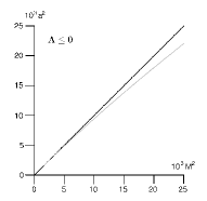
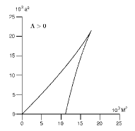
Analogously to the situation in Kerr space-time, we classify this form of the metric according to the number of (disconnected) regions where , which depends on the parameters , and . We speak of ‘slow‘ Kerr-de Sitter if there are two regions and of ‘fast‘ Kerr-de Sitter if there is one region where . The limiting case where two regions are connected by a zero is called ‘extreme‘ Kerr-de Sitter. Other cases are not possible, what can be seen by a comparison of coefficients in where denote the zeros of . Fig. 1 shows the modification of regions of slow, fast, and extreme Kerr-de Sitter with varying .
We can identify four constants of motion, two corresponding to the energy per unit mass and the angular momentum per unit mass in direction given by the generalized momenta and
| (9) | ||||
| (10) |
where the dot denotes a derivative with respect to the proper time . In addition, a third constant of motion is given by the normalization condition with for timelike and for lightlike geodesics. A fourth constant of motion can be obtained in the process of separation of the Hamilton-Jacobi equation
| (11) |
using the ansatz
| (12) |
If we insert this into (11) we get
| (13) |
where each side depends on or only. This means that each side is equal to a constant , the famous Carter constant, Carter (1968).
From the separation ansatz (12) we derive the equations of motion
| (14) | ||||
| (15) | ||||
| (16) | ||||
| (17) |
where and . The equations for and are coupled by . This difficulty can be overcome by introducing the Mino time Mino (2003) which is related to the proper time by . For simplicity, we rescale the parameters appearing in eqs. (14)-(17) such that they are dimensionless. Thus, we introduce
| (18) |
and accordingly
| (19) | ||||
In addition, we can absorb in the definition of by introducing
| (20) |
Then the equations (14)-(17) decouple and read
| (21) | ||||
| (22) | ||||
| (23) | ||||
| (24) |
where, as before,
| (25) | ||||
| (26) |
In section IV we will explicitly solve these equations.
III Types of timelike geodesics
Before solving the equations of motion derived in the previous section, we analyse the structure of possible orbits dependent on the black hole parameters , and the particle parameters . The major point in this analysis is that (21) and (22) imply and as a necessary condition for the existence of a geodesic. Although we concentrate here on timelike geodesics light can be treated in the same manner and is in general easier to deal with.
First of all, we state two short theorems about possible values of the Carter constant. The corresponding theorems for vanishing cosmological constant can be found in O’Neill (1995).
Theorem 1.
If a geodesic lies entirely in the equatorial plane or if it hits the ring singularity then the modified Carter constant is zero.
Proof.
A geodesic lies entirely in the equatorial plane iff for all . This implies that and with
it follows . If a geodesic hits the ring singularity, then there is a such that and . As and for all and , and in particular for , , it follows
and as above . ∎
Note that this theorem implies that is a necessary condition for equatorial orbits, which is an important class found in many astrophysical objects like accretion discs and planetary systems. Note that the modified Carter constant depends on the cosmological constant, which also influences the next theorem.
Theorem 2.
For all timelike and null geodesics have . In this case implies and the geodesic lies entirely in the equatorial plane.
Proof.
A geodesic can only exist if there are values for and with and . From it follows . If then and
for all values of . Assume now . Consequently
and only if and additionally . ∎
Since from observation the cosmological constant has a small positive value, the condition is always fulfilled.
From these two theorems it is obvious that, while originates from the separation procedure, the modified Carter constant has a geometric interpretation since it is related to possible values of the orbits. This relation will become more explicit in the following subsections.
In the remainder of the section we will study the consequences of the two conditions and .
III.1 Types of latitudinal motion
Geodesics can take an angle if and only if . Thus, we want to determine which values of , , , , , and result in positive . For simplicity, we substitute giving
| (27) |
Assume now that for a given set of parameters there exists a certain number of zeros of in . If we vary the parameters, the position of zeros varies and the number of real zeros in can change only if (i) a zero crosses or or (ii) two zeros merge. Let us consider case (i). is a zero iff
| (28) |
or
| (29) |
As is in general a pole of it is a necessary condition for being a zero of that this pole becomes a removable singularity. From (27) it follows that this is the case for or, equivalently, . Under this assumption we obtain
| (30) |
If we additionaly assume that (as in Thm. 2) we can conclude that iff and . Summarized, and simultaneously and (assuming ) give us boundary cases of the motion.
Now let us consider case (ii). If we exclude the coordinate singularities or the zeros of are given by the zeros of
| (31) |
which is in general a polynomial of degree . Then two zeros coincide at iff
| (32) |
for some real constants . By a comparison of coefficients we can solve this equation for and dependent the remaining parameters , and . This parametric representation of values of and again correspond to boundary cases of the motion. Let us additionally consider the conditions for being a double zero. With and (assuming ) it follows
| (33) |
which is zero for or, equivalently, .
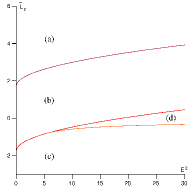
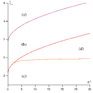
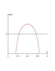
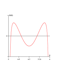
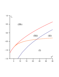
For given parameters of the black hole and , we can use these informations to analyse the motion of all possible geodesics in this space-time. As a typical example for timelike geodesics consider Fig. 2, where the curves divide the half plane into four regions (a)-(d) which correspond to different arrangement of zeros in . A geodesic motion is only possible in regions (b) and (d) because in all other regions is negative for all . Note that for the special case of (assuming ) strictly speaking regions (b) and (d) are divided by . However, in each region we have for and the same number of zeros in and, thus, the same type of motion. (More precisely, near a zero of approaches , but does not cross it.) Therefore, in each region we put the parts above and below together. The arrangement of zeros in the two regions (b) and (d) correspond to the following different types of motion in direction (cp. Fig. 3)
-
•
Region (b): has one real zero in with for , i.e. oscillates around the equatorial plane .
-
•
Region (d): has two real zeros in with for , i.e. oscillates between and .
The boundaries of region (b) are given by and, therefore, the regions gets larger if grows, i.e. if grows or gets smaller. A change of in addition causes region (b) to shift up or down. The dependence of region (d) on the parameters and is much more involved. The upper boundary of (d) is also the lower boundary of region (b). The lower boundary is given in a complicated parametric form which makes it apparently impossible to determine an explicit connection between the form of region (d) and the parameters. However, the point where the upper and lower boundaries of region (d) touch each other is where is a double zero of , which is given by in and from (32),
| (34) |
The regions (b) and (d) are characterized in a simple way in terms of the modified Carter constant . As in region (d) it follows that this region corresponds to because of . In the same way we can conclude that region (b), where , corresponds to .
III.2 Types of radial motion
A geodesic can take a radial coordinate if and only if . The zeros of are extremal values of and determine the type of geodesic. The polynomial is in general of degree six in and, therefore, has six possibly complex zeros of which the real zeros are of interest for the type of motion. As a Kerr-de Sitter space-time has no singularity in , we can also consider negative as valid. However, is an allowed value of iff
| (35) |
It follows that can only be crossed iff , which corresponds to region (d) of the motion. In region (b) of the motion where a transition from positive to negative is not possible.
To clarify the discussion we introduce some types of orbits O’Neill (1995).
-
•
Flyby orbit: starts from , then approaches a periapsis and back to .
-
•
Bound orbit: oscillates between to extremal with .
-
•
Transit orbit: starts from and goes to crossing .
All other types of orbits are exceptional and treated separately. They are either connected with the ring singularity or with the appearence of multiple zeros in , which simplifies the structure of the differential equation (21) considerably. Examples for the latter type are homoclinic orbits, cp. Levin and Perez-Giz (2009). As large negative correspond to negative mass of the black hole Hawking and Ellis (1973), we will assign the attribute ’crossover’ to flyby or bound orbits which pass from positive to negative or vice versa. (By definition, a transit orbit is always a crossover orbit and, therefore, we will not explicitly state that.) Therefore, in region (d) of the motion exists a crossover orbit, whereas all orbits located in region (b) of the motion do not cross .
For a given set of parameters we have a certain number of real zeros of . If we vary the parameters this number can change only if two zeros merge to one. This happens at iff
| (36) |
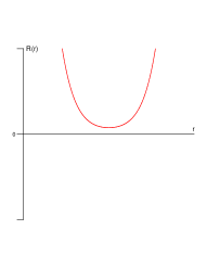
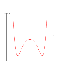
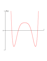
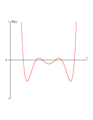
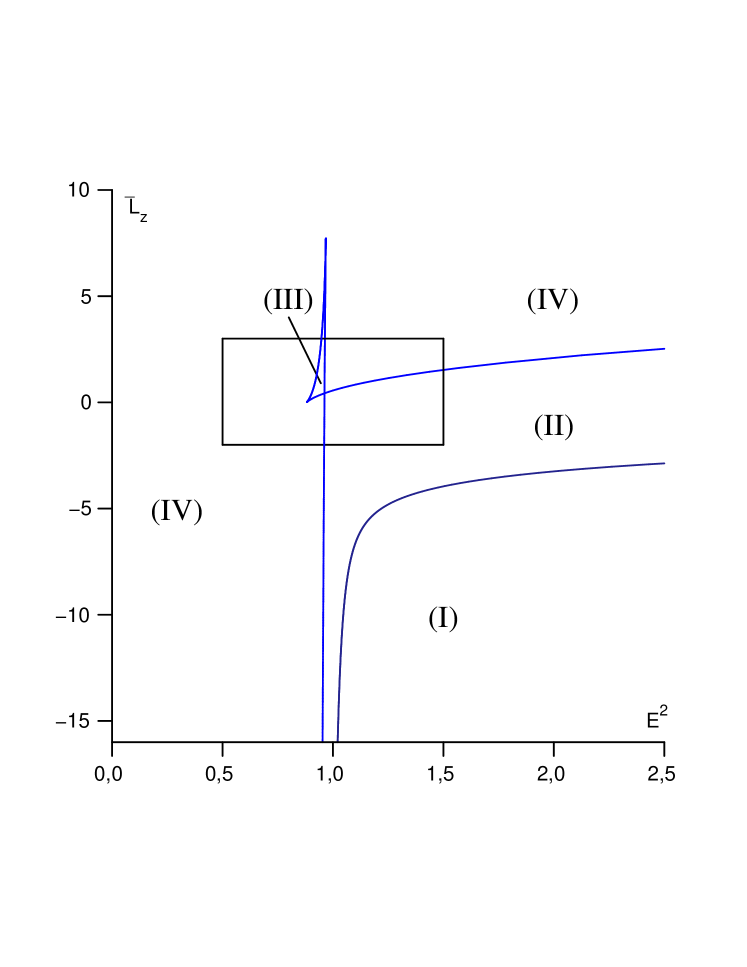
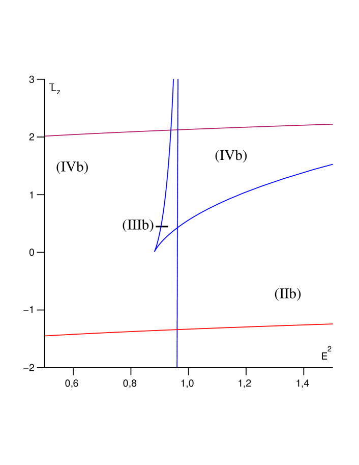
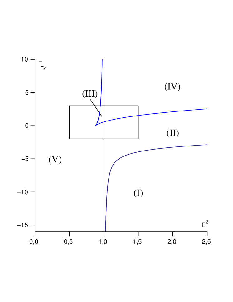
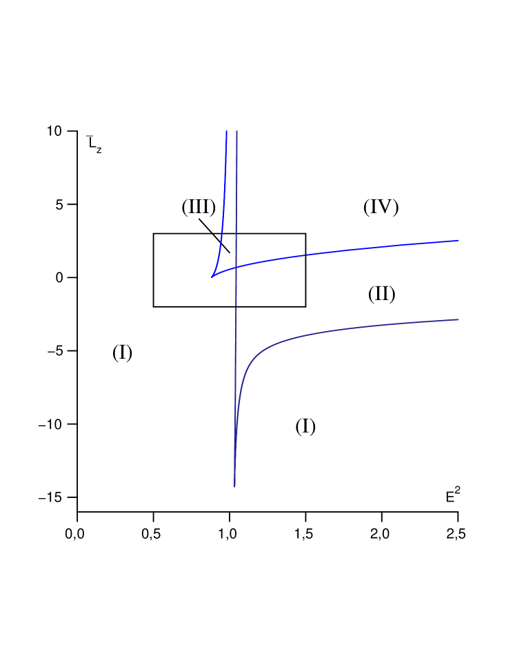
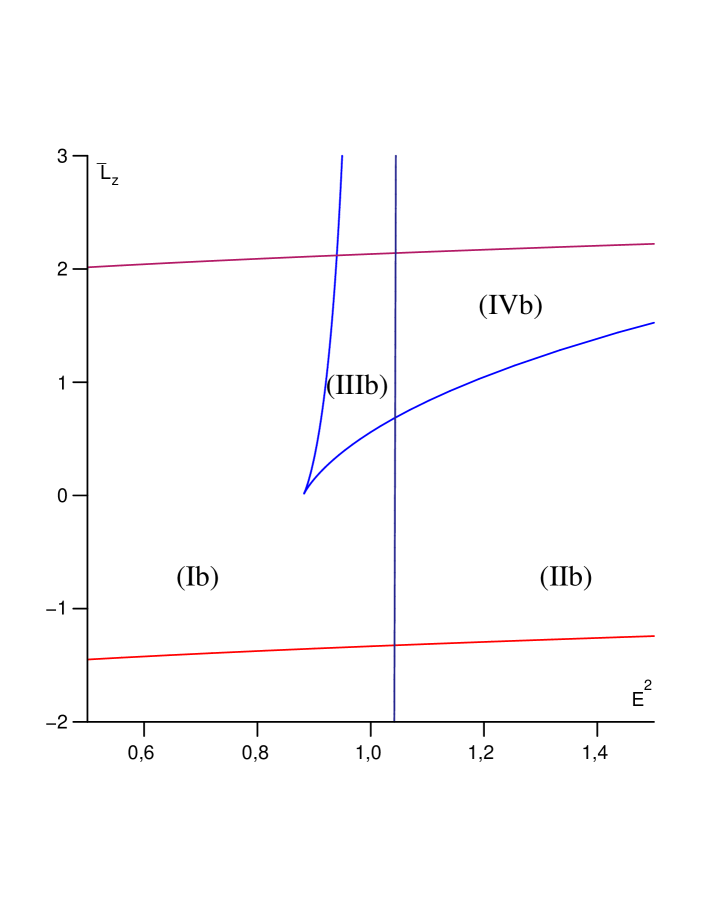
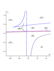
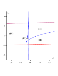
for some real constants . By a comparison of cofficients we can solve the resulting 7 equations for and dependent on the remaining parameters , , and . A typical result in slow Kerr-de Sitter for small including the results of the foregoing subsection is shown in Figs. 5 and 6. An analysis of the influence of each of the parameters , , and is not done easily due to the complexity of the expressions for and . However, some typical examples for varying are shown in Fig. 7. Examples of for different numbers of real zeros are given in Fig. 4.
We discuss now the resulting types of orbits. For simplicity, we restrict ourselves here to the case of slow Kerr-de Sitter although fast and extreme Kerr-de Sitter can be discussed analogously. This will be explicitly carried through in a future publication.
For comparison, let us first study the situation in slow Kerr with .
Case .
We recognize five regions of different types of motion. (Here we always assume .)
-
•
Region (I): all zeros of are complex and for all . Possible orbit types: transit orbit.
-
•
Region (II): has two real zeros and for and . Possible orbit types: two flyby orbits, one to and one to .
-
•
Region (III): all four zeros , , of are real and for , . Possible orbit types: two different bound orbits.
-
•
Region (IV): again all four zeros of are real but for , , and . Possible orbit types: two flyby orbits, one to each of and a bound orbit.
-
•
Region (V): has two real zeros and for . Possible orbit types: a bound orbit.
Although there are the same number of real zeros the different orbit types in regions (III)/(IV) and (II)/(V) is due to the different behaviour of when . For the expression is a polynomial of degree 4 with which for yields if and if .
Let us also analyse where we have crossover orbits. Region (II) is the only one which intersects region (b) as well as region (d) of motion. As region (I) can only contain a transit orbit, which is by definition a crossover orbit, it can only intersect region (d). All other regions contain only region (b) of motion and, therefore do not have any crossover orbits. The results of this paragraph together with the numbers of positive and negative zeros for each region are summarized in Tab. 1.
| region | + | range of | types of orbits | |
| Id | 0 | 0 | transit | |
| IIb | 1 | 1 | 2x flyby | |
| IId | 2 | 0 | flyby, | |
| crossover flyby | ||||
| IIIb | 0 | 4 | 2x bound | |
| IVb | 1 | 3 | 2x flyby, bound | |
| Vb | 0 | 2 | bound |
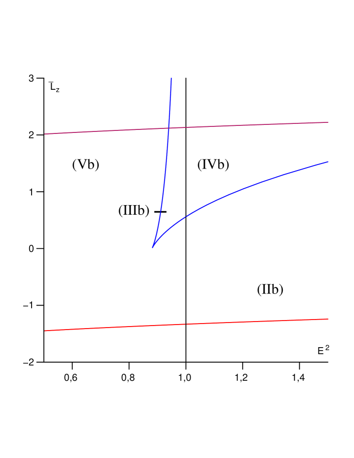
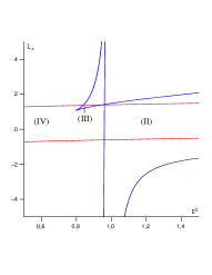
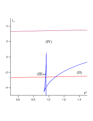
Case .
Let us analyse now which regions change compared to the case . At first, we recognize that region (V) for merged with region (IV) and that region (III) becomes smaller for due to the shift of the separating line towards the left. A comparison of the possible orbit types for with the one for shows that in regions (I) and (II) there are no differences. However, these regions are slightly deformed (for small ) and a pair of parameters located in region (I) or (II) for may be located in a different region for . We consider regions (III) and (IV). Here again we assume .
-
•
Region (III): all six zeros of are real and for and for . Possible orbit types: two flyby orbits, one to each of , and two different bound orbits.
-
•
Region (IV): has four real zeros and for . Possible orbit types: two flyby orbits, one to each of and a bound orbit.
Analogously to , regions (III) and (IV) only contain region (b) of motion implying that there are no crossover orbits. Region (I) can only intersect region (d) because only transit orbits are possible. The remaining region (II) is the only one which intersects regions (b) and (d).
We conclude that for the types of orbits are not noticeably changed, whereas for there are significant changes. In the former region (V) (for ), which is now in region (IV), and in region (III) we have two additional flyby orbits which are not present for . In a small vertical stripe left of there are even orbits which are bound for but reaching infinity for . In particular, it is independent of the value of if a geodesic may reach infinity as expected from the repulsive cosmological force related to .
Note that for huge the separation in regions (I) to (IV) is no longer possible because the repulsive cosmological force becomes so strong that bound orbits are no longer possible. In this case we have only two regions, one with two real zeros corresponding to two flyby orbits and one with only complex zeros corresponding to a transit orbit.
All orbit types for small are summarized in Tab. 2.
| region | + | range of | types of orbits | |
|---|---|---|---|---|
| Id | 0 | 0 | transit | |
| IIb | 1 | 1 | 2x flyby | |
| IId | 2 | 0 | flyby, | |
| crossover flyby | ||||
| IIIb | 1 | 5 | 2x flyby, 2x bound | |
| IVb | 1 | 3 | 2x flyby, bound |
Case .
Here region (V) from merges with region (I) and region (III) becomes larger for due to the shift of the line to the right. Compared to the situation for the possible orbit types in region (III) do not change, but a set of parameters located there may be located in a different region for . Let us examine the remaining regions.
-
•
Region (I): has two real zeros and for . Possible orbit types: bound orbit.
-
•
Region (II) (and (III)): has four real zeros with for , . Possible orbit types: two different bound orbits.
-
•
Region (IV): all six zeros of are real and for , . Possible orbit types: three different bound orbits.
Concerning crossover orbits regions (III) and (IV) again only contain region (b) of motion. Also region (II) intersects both (b) and (d) whereas region (I) can only contain region (d) of motion.
Summarizing, the types of orbits significantly change if . The transit orbit in region (I) for is transformed to a bound orbit for as well as the flyby orbits in regions (II) and (IV). Although region (V) for merges with region (I) for , the types of orbits do not change there. In general, because of if we can not have orbits reaching at all as expected due to the attractive cosmological force related to .
All orbit types for are summarized in Tab. 3
| region | + | range of | types of orbits | |
|---|---|---|---|---|
| Id | 1 | 1 | crossover bound | |
| IIb | 2 | 2 | 2x bound | |
| IId | 3 | 1 | bound | |
| crossover bound | ||||
| IIIb | 0 | 4 | 2x bound | |
| IVb | 2 | 4 | 3x bound |
IV Analytic solutions of the equations of motion
We will now analytically solve the geodesic equation in Kerr-de Sitter space-time (21) - (24). Each equation will be treated separately.
IV.1 motion
We begin with the differential equation (22)
which can be simplified by the substitution yielding
| (37) |
where is defined as in (31). This differential equation can be solved easily if has a zero with multiplicity or more. In this case (37) can be rewritten as
| (38) |
where and are initial values, is a polynomial with maximum degree , and is a zero of with multiplicity or , . The integral on the right hand side can then be solved by elementary functions Gradshteyn and Ryzhik (1983). As in this case the explicit expression provides no further insight and some case distinctions would be necessary we skip the solution procedure.
If has only simple zeros the differential equation (37) is of elliptic type and first kind and can be solved in terms of the Weierstrass elliptic function . In contrast to the motion considered in the next subsection, this structure does not simplify if we consider only light with . To obtain a solution we transform to the Weierstrass form for some constants and : First, we substitute giving
| (39) |
where
| (40) | ||||
Second, we substitute yielding
| (41) |
where
| (42) |
The differential equation (41) is elliptic of first kind, which can be solved by
| (43) |
Accordingly, the solution of (22) is given by
| (44) |
where with depends on the initial values and only. The sign of the square root depends on whether should be in (positive sign) or in (negative sign) and reflects the symmetry of the motion with respect to the equatorial plane . If the motion is located in region (b) from the previous section this implies that the two solutions have to be glued together along if the whole motion should be considered.
IV.2 motion
The differential equation that describes the dynamics of (21)
is more complicated because is a polynomial of a degree up to . If has a zero of multiplicity or more, or if has two zeros of multiplicity or more, the differential equation (21) can be written as
| (45) |
where and are initial values, is a polynomial with maximum degree 2, are zeros of with multiplicity or where , and if there are two zeros of multiplicity or more and else. The integral on the right hand side can then be solved by elementary functions Gradshteyn and Ryzhik (1983). As the explicit expression provides no further insight and some case distinctions would be necessary we skip the solution procedure.
If we consider null geodesics, i.e. , is in general of degree 4 and the differential equation (21) is of elliptic type and first kind. Then it can be handled using the method presented in the foregoing subsection: With the substitutions , where is a zero of , and , where , we arrive at a form (41). This can then again be solved in terms of Weierstrass elliptic functions. The result is
| (46) |
where with depends only on the initial values and and are defined as in (42) with .
The differential equation (21) is also of elliptic type but of third kind if has a double or triple zero . In this case (21) reads
| (47) |
where is a polynomial of degree 4. This equation can be solved for analogous to the method which will be presented in subsection IV.3.
If we consider particles, i.e. , and assume that has only simple zeros the differential equation (21) is of hyperelliptic type. It can be solved in terms of derivatives of the Kleinian function with the method developed in Hackmann and Lämmerzahl (2008a). For this, we have to cast (21) in the standard form by a substitution with a zero of . This yields
| (48) |
where
| (49) |
The sign in the substitution has be chosen such that the constant is positive and, therefore, depends on the choice of and the sign of . The differential equation (48) is of first kind and can be solved by
| (50) |
where and depends only on the initial values and . Here is the function that describes the -divisor, i.e. , cp. Hackmann and Lämmerzahl (2008a). The radial distance is then given by
| (51) |
where the sign depends on the sign chosen in the substitution , i.e. is such that in (49) is positive.
IV.3 motion
We treat now the most complicated equation of motion in Kerr-de Sitter space-time, namely the equation for the azimuthal angle (23)
This equation can be splitted in a part dependent only on and in a part only dependent on . Integration yields
| (52) |
where we substituted , i.e. , in the first and , i.e. , in the second integral.
We will solve now the two integrals in (52) separately.
IV.3.1 The dependent integral
Let us consider the integral
| (53) |
which can be transformed to the simpler form
| (54) |
by the substitution , where is defined in (31) and . Here we have to pay special attention to the integration path. If we have but for it is . Accordingly, we first have to split the integration path from to such that every piece is fully contained in the interval or and then to choose the appropiate sign of the square root of . In the following we assume for simplicity that .
Analogous to subsection IV.1 the integral can be solved by elementary functions if has at least a double zero Gradshteyn and Ryzhik (1983). If has only simple zeros is of elliptic type and of third kind. If this is the case, the solution to is given by
| (55) |
where the constants are defined as in subsection IV.1, , , with as in (43) and . The integers correspond to different branches of . The details of the computation can be found in appendix A.
IV.3.2 The dependent integral
We solve now the first, dependent integral in (52)
| (56) |
Analogous to subsection IV.2 this integral can be solved by elementary functions if has a zero with multiplicity or more or two zeros with multiplicity or more Gradshteyn and Ryzhik (1983).
If we consider light, i.e. , is in general of degree and is of elliptic type and third kind. In this case it can be solved analogously to . The same substitutions and as in subsection IV.2 for the case , a subsequent partial fraction decomposition, and the final substitution result in
| (57) |
where are the four zeros of , defined as in (46), and are the coefficients of the partial fractions dependent on the parameters and . The four functions have simple poles in with and have to be integrated wih the method presented in appendix A. Then is given by
| (58) |
where , with as in (46). In the same way can be solved if has a double or triple zero.
If we consider particles, i.e. , and assume that has only simple zeros, is of hyperelliptic type and third kind. The details of the solution method can be found in appendix B but we give an outline here: First, we transform analogously to section IV.2 to the standard form by with a zero of . Afterward we simplify the integrand by a partial fraction decomposition which allows us to express in terms of the canonical holomorphic differentials (91) and the canonical differential of third kind (88). These differentials can then be expressed in dependence of the normalized Mino time . If we define and the result is
| (59) |
where the constants are the coefficients of the partial fractions, are the four zeros of , , and and as in (48). The functions are defined by , where the points on the Riemann surface of are the pole located on the positive and the negative branch of the square root.
IV.4 motion
The equation for (24)
is as complicated as the equation for motion. An integration yields
| (60) |
Because we already demonstrated the solution procedure, we only give here the results for the most general cases.
If in (37) has only simple zeros the solution of the dependent part is given by
| (61) |
If we consider light, i.e. , the solution for the dependent part is given by
| (62) |
where is defined as in (46), are the coefficients of the partial fractions, with the four zeros of , and , as in (46).
If has only simple zeros and we consider timelike geodesics the solution of the dependent part is given by
| (63) |
where the notation is as in (59) and are the coefficients of the partial fractions.
V Discussion of some geodesics
In Sec. III we discussed the general features of the different types of timelike geodesic motion in Kerr-de Sitter and Kerr-anti-de Sitter space-time. With the analytical solution derived in section IV at hand we want to discuss now some chosen geodesics.
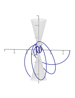
We start with orbits which highlight the influence of on the geodesics. From the results of section III we conclude that for there are four parameter regions where the changes compared to are most obvious. The first two are the regions (III) and (IV) with , where we have additional flyby orbits not present for . Third and fourth, the shift from region (V) of to region (II) of for , small, and the shift from region (III) of to region (IV) of , again for are most interesting as the (outer) bound orbit becomes a flyby orbit. A plot of the corresponding orbits can be found in Fig. 8.

(region (IVb))
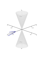
(region(IIIb))
(region (IIb))
(region (IVb)
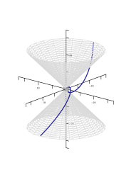
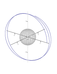
An important feature of geodesics in stationary axisymmetric space-times is motion of the nodes where the orbit of a test-particle or light intercepts the equatorial plane. This motion is caused by the components of the space-time metric and known as the Lense-Thirring effect. In the weak field regime it becomes visible by a precession of the orbital plane, cp. Fig. 9 for an obvious example. This orbital precession has been confirmed within an accuracy of about 10% by the LAGEOS (Laser Geodynamics Satellite) mission Ciufolini (2007), 111Another method to observe the influence of the gravitomagnetic components is through the precession of gyroscopes known also as Schiff effect. Such a measurement has been carried through by Gravity Probe B F. Everitt et al. (2009). While the Lense-Thirring effect is an orbital effect involving the motion of the whole orbit thus constituting a global measurement, the Schiff effect is a local effect showing the dragging of local inertial frames due to the existence of the components..
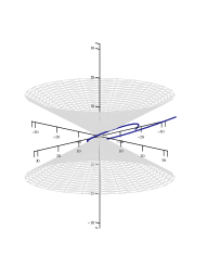
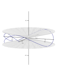
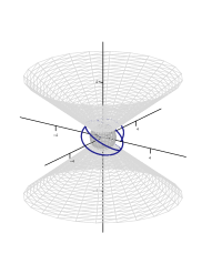
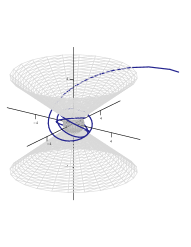
Let us also discuss some exceptional orbits related to multiple zeros of , i.e. spherical orbits with constant and orbits asymptotically approaching a constant . There are two types of spherical orbits: stable and unstable. Stable spherical orbits with occur if radial coordinates adjacent to are not allowed due to , which happens if is a maximum of . Unstable spherical orbits with are trajectories where radial coordinates in the neighbourhood of with or are allowed. Therefore, these orbits are related to a minimum or to an inflection point of . If is an inflection point, an asymptotic approach to is only possible from one side of whereas this is possible from both sides if is a minimum of . Asymptotic orbits can also be devided into two types: unbound and bound. The latter case corresponds to orbits which approach for both and a spherical orbit. Bound asymptotic orbits are also known as homoclinic orbits. If the asymptotic orbit is unbound it reaches for either or .
For asymptotic bound or unbound trajectories corresponding to an unstable spherical orbits the equations of motion simplify considerably. In this case the equation for as well as the dependent integrals in the and equations are of elliptic type and can be solved in terms of Weierstrass elliptic functions, see (47) and (58). Note that these solutions are not limited to the case of equatorial circular orbits but are valid for all types of asymptotic orbits and, thus, generalize the analytical solutions for homoclinic orbits in Levin and Perez-Giz (2009) not only to Kerr-de Sitter space-time but also to arbitrary inclinations.
From all spherical orbits the Last Stable Spherical Orbit (LSSO), in particular, the Innermost Stable Circular Orbit (ISCO) in the equatorial plane are of importance as they represent the transition from stable orbits to those which fall through the event horizon. The corresponding multiple zero of appears at the boundaries of the different regions of motion, cp. Fig. 5. Because necessarily for equatorial orbits, from this we can determine the LSSO for given , , and the ISCO for given , by solving first
| (64) |
for with the event horizon . The solutions are limiting cases of the LSSO or ISCO and are given by the corner points on the borders of region (III) of the motion (as corners on other boundaries correspond to ). From the results of (64) we search for the smallest possible double zero which is a maximum. In the case of the ISCO in the equatorial plane we are now done. For the LSSO, we have to check in addition whether the corresponding values of and (given by (36)) are located in an allowed region of the motion. If this is the case, we found the LSSO. If not, we can determine the LSSO as the intersection point of the boundary of region (III) with a boundary of an allowed region. Note that it is not possible to determine an LSSO (for given , , and ) if there is no spherical orbit at all outside the event horizon which happens if no boundary of the motion is located in an allowed region of the motion. As an example, this is the case for , , and . Also, the LSSO is identical with the ISCO if it is given as an intersection point with the boundary of region (b) of the motion. For examples of spherical orbits see Figs. 10 and 11. Note that within the event horizon there may be additional stable spherical orbits.
VI Analytic expressions for observables
For the understanding of characteristic features of space-times by measurements of geodesics in that space-time it is crucial to identify certain theoretical quantities of observables. For flyby orbits, this can be the deflection angle of the geodesic whereas for bound orbits it is of interest to determine the orbital frequencies as well as the periastron shift and the Lense-Thirring effect.
Let us first consider flyby orbits. The deflection angle of such an orbit depends on the two values of the normalized Mino time for which . These are given by
| (65) |
for the two branches of . Therefore, we can calculate the values of and for that are taken by this flyby orbit by and . The deflection angles are then given by and .
For bound orbits we can identify three orbital frequencies , and associated with the coordinates , and . The precessions of the orbital ellipse, which in the weak field regime can be identified with the periastron shift, and the orbital plane, which in the weak field regime can be identified with the Lense-Thirring effect, are induced by mismatches of these orbital frequencies. More precisely, the orbital ellipse precesses at and the orbital plane at .
Let us consider the orbital frequency . For bound orbits the coordinate is contained in an intervall with the peri- and apoapsis distances and . The orbital period defined by is then given by a complete revolution from to and back (with reversed sign of the square root) to ,
| (66) |
The orbital frequency of the motion with respect to is then given by . For the calculation of , which represents the orbital frequency with respect to , we need in addition the average rate at which accumulates with . This will be determined below.
For the calculation of the orbital frequency we have to determine the orbital period such that . The motion is likewise bounded by for two real zeros of and, therefore,
| (67) |
Again, the orbital frequency of the motion with respect to is given by .
The orbital periods of the remaining coordinates and has to be treated somewhat differently because they depend on both and . The solutions and consist of two different parts, one which represents the average rates and at which and accumulate with and one which represents oscillations around it with periods and Drasco and Hughes (2004); Fujita and Hikada (2009). The periods and can be calculated by Fujita and Hikada (2009)
| (68) | ||||
| (69) |
The orbital frequencies , , and are then given by
| (70) |
If the integral expressions for and the dependent parts of and degenerate to elliptic or elementary type, i.e. if we consider light or possesses multiple zeros, we can find analytical expressions for (66), (68), and (69) with the techniques presented in Fujita and Hikada (2009). If has only simple zeros and , the integral is an entry of the fundamental period matrix which enters in the definition of the period lattice of the holomorphic differentials , . The more complicated integrals involving in (68) and (69) can be rewritten in terms of periods of the differentials of second kind and of third kind by a decomposition in partial fractions. In this way, expressions for , and which are totally analogous to the elliptic case can be obtained.
It follows that the periastron shift is given by
| (71) |
and the Lense-Thirring effect by
| (72) |
Another way to access information encoded in the orbits is through a frequency decomposision of the whole orbit Drasco and Hughes (2004). This will be analyzed elsewhere.
VII Summary and outlook
In this paper we derived the analytical solution for both timelike and lightlike geodesic motion in Kerr-(anti-)de Sitter space-time. The analytical expressions for the orbits are given by elliptic Weierstrass and hyperellliptic Kleinian functions in terms of the normalized Mino time. We also presented a method for solving differential equations of hyperelliptic type and third kind, and applied it to the equations of motion for and . We classified possible types of geodesic motion by an analysis of the zeros of the polynomials underlying the and motion and discussed the influence of a non-vanishing cosmological constant on the orbit types. Some particular interesting orbits not present in Kerr space-time were shown and a systematic approach for determining the last stable spherical and circular orbits was presented. In addition, we derived the analytic expressions for observables connected with geodesic motion in Kerr-de Sitter space-time, namely the deflection angle for escape orbits as well as the orbital frequencies, the periastron shift, and Lense-Thirring effect of bound orbits.
The results of this paper can be viewed as the starting point for the analysis of several features of geodesics in Kerr-de Sitter space-time not treated in this publication. Although mathematical analogous to the case of slow Kerr-de Sitter a complete discussion of orbits in fast and extreme Kerr-de Sitter space-times may lead to special features and should be carried through. Also, it would be interesting to study bound geodesics crossing (and mayby also the Cauchy horizon for positive ) in general and, in particular, their causal structure. In this context the analysis of closed timelike trajectories is also of interest. In addition, we not yet considered geodesics lying entirely on the axis or even crossing it. Until now, we only considered the Boyer-Lindquist form of the Kerr-de Sitter metric which is not a good choice for considering geodesics which fall through a horizon. Therefore, for a future publication it would be interesting to use a coordinate-singularity free version of the metric.
The methods for obtaining analytical solutions of geodesic equations presented in this paper are not only limited to Kerr-de Sitter space-time. Indeed, they had already been used to solve the geodesic equation in Schwarzschild-de Sitter Hackmann and Lämmerzahl (2008a, b) and Reissner-Nordström-de Sitter Hackmann et al. (2008) space-times. Also the geodesic equations in higher-dimensional static spherically symmetric space-times Hackmann et al. (2008) were solved by these methods. The same type of differential equations is also present in the Plebański-Demiański space-time without acceleration, which is the most general space-time with separable Hamilton-Jacobi equation. The analytical solution of the geodesic equation in this space-time is given in Hackmann et al. (2009) but will be elaborated in an upcoming publication. It will also be interesting to apply the presented methods to higher dimensional stationary axially symmetric space-times like the Myers-Perry solutions.
The same structure of equations we solved in this paper is also present in the geodesic equation of the effective one-body formalism of the relativistic two-body problem. The effective metric in this formalism can be described as a perturbed Schwarzschild or Kerr metric, where the pertubation is given in powers of the radial coordinate Damour (2001); Damour et al. (2008a, b). Therefore, we expect that the polynomial appearing in the resulting equations of motion will have a higher degree than the corresponding polynomial in the Schwarzschild or Kerr case and, thus, that it is necessary to generalize the elliptic functions used in these cases to hyperelliptic functions used in this paper. A similar situation can be found in the expressions of axisymmetric gravitational multipole space-times. For example, some types of geodesics in Erez-Rosen space-time, which reduces to the Schwarzschild case if the quadrupole moment is neglected, were already solved analytically Quevedo (1990, 1989). We expect that the methods presented in this paper will be helpful to solve geodesics in space-times with multipoles.
Analytic solutions are the starting point for approximation methods for the description of real stellar, planetary, comet, asteroid, or satellite trajectories (see e.g. Hagihara (1970)). In particular, it is possible to derive post-Kerr, post-Schwarzschild, or post-Newton series expansions of analytical solutions. Due to the, in principle, arbitrary high accuracy of analytic solutions of the geodesic equation they can also serve as test beds for numerical codes for the dynamics of binary systems in the extreme stellar mass ratio case (extreme mass ratio inspirals, EMRIs) and also for the calculation of corresponding gravitational wave templates. For the case of Kerr space-time with vanishing cosmological constant it has already been shown that gravitational waves from EMRIs can be computed more accurately by using analytical solutions than by numerical integration Fujita and Hikada (2009).
Due to the high precission, the analytical expressions for observables in Kerr-de Sitter space-time may be used for comparisons with observations where the influence of the cosmological constant might play a role. This could be the case for stars moving around the galactic center black hole or binary systems with extreme mass ratios where one body serves as test-particle. For example, quasar QJ287 (cp. M.J. Valtonen et al. (2008)) could be a candidate for observing the effects of a non-vanishing cosmological constant. In this context it would also be interesting for a future publication to derive post-Kerr, post-Schwarzschild, or post-Newton expressions for observables.
Acknowledgements.
We are grateful to H. Dullin, W. Fischer, and P. Richter for helpful discussions. V.K. thanks the German Academic Exchange Service DAAD and E.H. the German Research Foundation DFG for financial support.Appendix A Integration of elliptic integrals of the third kind
In this appendix we will demonstrate the details of the integration method of the elliptic integrals of third kind which appear in the dependent part of the and motion (52), (60) and in the special case of the motion where has a double or triple zero. We will explain the procedure for the example of the integral in (52). As this integral is only elliptic if has only simple zeros we assume in the following that this is the case.
Before we demonstrate the calculational steps, we will summarize them for convenience:
-
1.
Cast the expression under the square root in the standard Weierstrass form for some constants , the so-called Weierstrass invariants.
-
2.
Decompose the integrand (without the square root) in partial fractions.
-
3.
Substitute .
-
4.
For every partial fraction, rewrite the integrand in terms of the Weiertsrass (double pole) or function (simple pole).
-
5.
Integrate the Weierstrass and functions and assemble all parts.
Let us start from eq. (54)
where we assumed that the original integration path was fully contained in . With the substitutions and , as in subsection IV.1, we obtain
| (73) |
where is defined in (40), are defined as in (42), , and . Now we simplify the integrand in (73) (without the square root) by a partial fraction decomposition
| (74) |
where . With the substitution we can get rid of the square root in (73) as where the sign has to be chosen according to the sign of and the branch of the square root. The function is negative for and positive for where and are the fundamental periods of . As corresponds to we will have in most cases.
Altogether, the integral now reads
| (75) |
The second and third integral are of third kind because and have simple poles. We will rewrite now and in terms the Weierstrass -function, which has a simple zero in . The reason is, that can easily be integrated in terms of the Weierstrass -function
| (76) |
We only demonstrate the procedure for which is totally analogous to the procedure for . The function has two simple poles and lying in the fundamental domain , where and as above, with . An expansion of and in neighbourhoods of yields
| (77) | ||||
| (78) |
for some constants . Now a comparison of coefficients gives
| (79) |
It follows that the function is an elliptic function without poles and, therefore, equal to a constant which can be determined by . This yields and
| (80) |
Note that . The expression for can be determined by the differential equation , where again the sign of the square root has to be chosen according to the sign of . An intergation of yields
| (81) |
In the same way we can integrate , where we assume that and are the simple poles of in the fundamental domain with . Summarized, is given by (cp. (55))
where by (43) and . The integers correspond to different branches of .
Appendix B Integration of hyperelliptic integrals of the third kind
In this appendix we will demonstrate the details of the integration method of the hyperelliptic integrals of third kind which appear in the dependent part of the and motion (52), (60). We will explain the procedure for the example of the integral in (52). As this integral is only hyperelliptic if we consider timelike geodesics, i.e. and has only simple zeros we assume in the following that this is the case.
Before we demonstrate the solution steps, we will summarize them for convinience:
-
1.
Cast the expression under the square root in the standard form for some constants .
-
2.
Decompose the integrand (without the square root) in partial fractions.
-
3.
If integrals of first or second kind are present, rewrite them as functions of .
-
4.
Rewrite the integrals of third kind in terms of the canonical integral of third kind .
-
5.
Rewrite the canonical integrals of third kind in terms of the Kleinian sigma functions, such reducing them to functions of integrals of first kind.
-
6.
Express the integrals of first kind in terms of and assemble all parts.
Let us start with eq. (56)
which can analogously to section IV.2 be transformed to the standard form by with a zero of and get
| (82) |
where and are defined as in section IV.2 and , i.e.
| (83) |
which is a polynomial of degree 4 in . Note that for geodesic motion, the coordinate is always contained in an interval bounded by two adjacent real zeros of the polynomial or by a real zero and infinity. This implies that for a real zero of does not change sign on the integration path and, therefore, we can neglect the absolute value of appearing in the integrand if we multiply the hole integral with . Consequently
| (84) |
The expression for the integrand in (84) can be simplified by a partial fraction decomposition
| (85) |
where , denote the zeros of and are quite complicated expressions dependent on the parameters and the zero of which may be calculated by a Computer Algebra System.
The first two integrals in this expression are of first kind and can be solved analogous to section IV.2 (48), i.e.
| (86) | ||||
| (87) |
where again with only depends on the initial values and , and describes the -divisor, i.e. .
The four integrals in (85) containing are in general of third kind and can be expressed in terms of the canonical integral of third kind . The most simple construction of a differential of third kind
| (88) |
has simple poles in the points and of the Riemann surface of , a polynomial, with residual and , respectively (cp. Buchstaber et al. (1997); Baker (1907)). In particular, we get
| (89) |
where is the pole located on the positive branch of the square root and is the pole located on the negative branch of the square root. Based on Riemann’s vanishing theorem (see e.g. Buchstaber et al. (1997)) the canonical differential of third kind can be expressed in terms of Kleinian functions by
| (90) |
where is the vector of canonical differentials of the first kind and the vector of canonical differentials of the second kind
| (91) | ||||
| (92) |
Finally, we rewrite (90) in terms of the affine parameter . By (86) and (87) we can express as well as the arguments of the functions as functions of . If we define and the integral is given by (cp. (59))
where and .
References
- Dunkley et al. (2009) Dunkley et al., Astrophys. J. Suppl. 180, 306 (2009).
- Jetzer and Sereno (2006) P. Jetzer and M. Sereno, Phys. Rev. D 73, 044015 (2006).
- Kerr et al. (2003) A. Kerr, J. Hauck, and B. Mashhoon, Class. Qauntum Grav. 20, 2727 (2003).
- Kagramanova et al. (2006) V. Kagramanova, J. Kunz, and C. Lämmerzahl, Phys. Lett. A 634, 465 (2006).
- Anderson et al. (2002) J. Anderson, P. Laing, E. Lau, A. Liu, M. Nieto, and S. Turyshev, Phys. Rev. D 65, 082004 (2002).
- Sanders (1996) R. Sanders, Astrophys. J. 473, 117 (1996).
- Näf et al. (2009) J. Näf, P. Jetzer, and M. Sereno, Phys. Rev. D 79, 024014 (2009).
- Barabèz and Hogan (2007) C. Barabèz and P. Hogan, Phys. Rev. D 75, 124012 (2007).
- Dexter and Agol (2009) J. Dexter and E. Agol, Astrophys. J. 696, 1616 (2009).
- Hagihara (1931) Y. Hagihara, Japan. J. Astron. Geophys. 8, 67 (1931).
- Chandrasekhar (1983) S. Chandrasekhar, The Mathematical Theory of Black Holes (Oxford University Press, Oxford, 1983).
- Kraniotis (2004) G. Kraniotis, Class. Quantum Grav. 21, 4743 (2004).
- Fujita and Hikada (2009) R. Fujita and W. Hikada, Class. Quantum Grav. 26, 135002 (2009).
- Hackmann and Lämmerzahl (2008a) E. Hackmann and C. Lämmerzahl, Phys. Rev. Lett. 100, 171101 (2008a).
- Hackmann and Lämmerzahl (2008b) E. Hackmann and C. Lämmerzahl, Phys. Rev. D 78, 024035 (2008b).
- Enolskii et al. (2003) V. Enolskii, M. Pronine, and P. Richter, J. Nonlinear Sc. 13, 157 (2003).
- Hackmann et al. (2008) E. Hackmann, V. Kagramanova, J. Kunz, and C. Lämmerzahl, Phys. Rev. D 78, 124018 (2008).
- Hackmann et al. (2009) E. Hackmann, V. Kagramanova, J. Kunz, and C. Lämmerzahl, Europhys. Lett. 88, 30008 (2009).
- Mino (2003) Y. Mino, Phys. Rev. D 67, 084027 (2003).
- Carter (1968) B. Carter, Phys. Rev. 174, 5, 1559 (1968).
- O’Neill (1995) B. O’Neill, The Geometry of Black holes (A K Peters, Wellesly, Massasuchetts, 1995).
- Levin and Perez-Giz (2009) J. Levin and G. Perez-Giz, Phys. Rev. D 79, 124013 (2009).
- Hawking and Ellis (1973) S. W. Hawking and G. Ellis, The large scale structure of space-time (Cambridge Univ. P., Cambridge, 1973).
- Gradshteyn and Ryzhik (1983) I. Gradshteyn and I. Ryzhik, Table of Integrals, Series, and Products (Academic Press, Orlando, 1983).
- Ciufolini (2007) I. Ciufolini, Nature 449, 41 (2007).
- Drasco and Hughes (2004) S. Drasco and S. Hughes, Phys. Rev. D 69, 044015 (2004).
- Damour (2001) T. Damour, Phys.Rev. D 64, 124013 (2001).
- Damour et al. (2008a) T. Damour, P. Jaranowski, and G. Schäfer, Phys. Rev. D 77, 064032 (2008a).
- Damour et al. (2008b) T. Damour, P. Jaranowski, and G. Schäfer, Phys.Rev. D78, 024009 (2008b).
- Quevedo (1990) H. Quevedo, Fortschr. Phys. 38, 733 (1990).
- Quevedo (1989) H. Quevedo, Phys. Rev. D 39, 2904 (1989).
- Hagihara (1970) Y. Hagihara, Celestial Mechanics (MIT Press, Cambridge, Mass., 1970).
- M.J. Valtonen et al. (2008) M.J. Valtonen et al., Nature 452, 851 (2008).
- Buchstaber et al. (1997) V. Buchstaber, V. Enolskii, and D. Leykin, Hyperelliptic Kleinian Functions and Applications, Reviews in Mathematics and Mathematical Physics 10 (Gordon and Breach, 1997).
- Baker (1907) H. Baker, Multiply Periodic Functions (Cambridge University Press, 1907).
- F. Everitt et al. (2009) F. Everitt et al., Space Sci. Rev. (2009), in print, online DOI 10.1007/s11214-009-9524-7.