Performance Analysis of the Matrix Pair Beamformer with Matrix Mismatch

Jianshu Chen, , Jian Wang,  Xiu-Ming Shan, 
Ning Ge,   and Xiang-Gen Xia, 
EDICS: SAM-PERF
This work was supported by the National Natural Science Foundation of China under contract No. 60972019 and No. 60928001. Jianshu Chen was with the Department of Electronic Engineering, Tsinghua University, Beijing, P. R. China, 100084. He is with the Department of Electrical Engineering, University of California, Los Angeles, CA 90095, USA. (e-mail: jshchen@ee.ucla.edu) Jian Wang, Xiu-Ming Shan and Ning Ge are with the Department of Electronic Engineering, Tsinghua University, Beijing, P. R. China, 100084. (e-mail: {jian-wang, shanxm, gening} @tsinghua.edu.cn) Xiang-Gen Xia is with the Department of Electrical and Computer Engineering, University of Delaware, Newark, DE 19716, USA. (e-mail: xxia@ee.udel.edu). His work was suppported in part by the Air Force Office of Scientific Research (AFOSR) under Grant No. FA9550-08-1-0219, the National Science Foundation (NSF) under Grant CCF-0964500, and the World Class University (WCU) Program 2008-000-20014-0, National Research Foundation, Korea.
Abstract

Matrix pair beamformer (MPB) is a blind beamformer. It exploits the temporal structure of the signal of interest (SOI) and applies generalized eigen-decomposition to a covariance matrix pair. Unlike other blind algorithms, it only uses the second order statistics. A key assumption in the previous work is that the two matrices have the same interference statistics. However, this assumption may be invalid in the presence of multipath propagations or certain “smart” jammers, and we call it as matrix mismatch. This paper analyzes the performance of MPB with matrix mismatch. First, we propose a general framework that covers the existing schemes. Then, we derive its normalized output SINR. It reveals that the matrix mismatch leads to a threshold effect caused by “steering vector competition”. Second, using matrix perturbation theory, we find that, if there are generalized eigenvalues that are infinite, the threshold will increase unboundedly with the interference power. This is highly probable when there are multiple periodical interferers. Finally, we present simulation results to verify our analysis.

Index Terms:
Adaptive beamforming, Matrix pair beamformer, Generalized eigen-decomposition, Matrix mismatch

I Introduction

Beamforming is a spatial filter, which combines the outputs of multiple sensor elements by an appropriately designed weight vector so as to pass a signal of interest (SOI) while rejecting interfering signals. Since the pioneering work of Howells[1], Applebaum[2] and Widrow[3], it has been intensively studied during the past decades and widely applied in radar, sonar and wireless communications [3, 4, 5, 6, 7, 8, 9, 10, 11] etc. For a comprehensive review, we refer to [12, 13, 14, 15] and the references therein.

There are various forms of implementations for a beamformer. Some use the direction of arrival (DOA) of the SOI and directly calculate the weight vector by sample matrix inversion (SMI) [16]. Some employ a reference signal (e.g. training signal[17] and decision feedback signal[6]) to iteratively calculate the weight vector. And there are also blind beamformers which do not require the DOA or the reference signal[18, 19, 20, 21, 22, 23, 24, 25, 26, 27, 28, 29, 30, 31].

To achieve blind beamforming, we need to exploit the special properties of the SOI, such as constant modulus, non-Gaussianness, high order statistics etc. One important property is the temporal structure of the SOI. Such kind of blind beamformers are extensively studied for CDMA systems, where the inherent structure of the spreading codes can be exploited[23, 24, 25, 26, 28, 29, 30, 31]. The advantage of this scheme is that it only relies on the second order statistics of the covariance matrix pair. Although the implementation details differ, the main idea of these approaches is to exploit a pair of array covariance matrix and hence will be referred to as matrix pair beamformer (MPB) in this paper. The MPB projects the discrete sequence in each antenna onto the space spanned by the SOI’s signature vector (for a CDMA system, it is the spreading code vector) and another carefully designed base vector. Then two sets of array snapshots (i.e. signal snapshot and interference snapshot) are acquired to calculate a pair of covariance matrices. With the processing gain, the desired signal power in the signal snapshot is generally greater than that in the interference snapshot. A key and common assumption is that the interference statistics in the two snapshots are identical. These two features enable the separation of the signal steering vector and the interference covariance matrix from the two matices. And the weight vector derived from the dominant eigenvector of the matrix pair will maximize the output signal to interference plus noise ratio (SINR).

However, this key assumption that the two matrices share the same interference statistics is not valid in many cases, which we refer to as matrix mismatch. Matrix mismatch may occur when there are interferers with certain periodical structure, such as multiple access interference (MAI) in CDMA systems, tones and some other “smart jammers” in radar systems and it may lead to the failure of a system. In practical applications, to avoid such an unexpected failure, it is necessary to understand the detailed performance of a scheme when the assumption/condition is not satisfied. To our best knowledge, little effort has been devoted to analyzing the effect of matrix mismatch on the performance of MPB. This paper aims to analyze the MPB’s performance under matrix mismatch, and our contributions are:

  • proposing a general framework to model various existing MPB schemes;

  • deriving analytical expressions for the normalized output SINR as the performance measure;

  • discovering a threshold effect for MPB, i.e., due to matrix mismatch, the performance of MPB degrades rapidly when the input signal to noise ratio (SNR) is below a predicted threshold, and the main beam points to the directions of the interferers;

  • explaining how MPB works “blindly” by “steering vector competition”;

  • discussing various factors that have impact on the threshold, and showing that when there is an generalized eigenvalue that is infinite which is called the noise-free covariance matrix pair, the threshold SNR increases unboundedly with the interference power;

  • discussing several typical scenarios and showing that MPB is very vulnerable to multiple periodical interferers.

The rest of the paper is organized as follows. Sec. II presents a general framework of MPB to cover and reinterpret the basic ideas in [23, 24, 25, 26, 27, 28, 29, 30, 31], followed by a formulation of the matrix mismatch problem. In Sec. III, we present the expressions for MPB’s weight vector and its normalized output SINR, which uncovers the inherent threshold effect caused by matrix mismatch. The discussion relies heavily on the approximation of the generalized eigenvalue, which is derived in Appendix A using Gerschgorin theorem[32, 33]. Sec. IV applies the Weyl-Lidskii type theorem in matrix perturbation theory[32] to analyze MPB’s threshold SNR, and discusses it in two typical scenarios. Finally, Sec. V presents simulation results to verify our theoretical analysis and Sec. VI concludes the whole paper.

II Problem Formulation

II-A Signal Model
Refer to caption
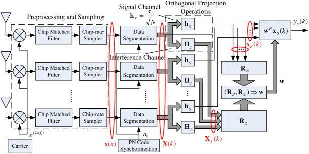
Figure 1: Block diagram of the matrix pair beamformer in a CDMA system. Data corresponding to the k𝑘k symbol are blocked and projected onto two spaces to produce signal channel snapshot 𝐱𝒮(k)subscript𝐱𝒮𝑘\mathbf{x}_{\mathcal{S}}(k) and interference channel snapshot 𝐗(k)subscript𝐗𝑘\mathbf{X}_{\mathcal{I}}(k), respectively.

Consider an antenna array of L𝐿L isotropic elements that receives D+1𝐷1D+1 signals from a far field. After preprocessing (e.g. mixing, filtering, etc.) and sampling, the output L×1𝐿1L\times 1 array vector can be written as

𝐱(n)=i=0DPisi(n)𝐚i+𝐯(n),𝐱𝑛superscriptsubscript𝑖0𝐷subscript𝑃𝑖subscript𝑠𝑖𝑛subscript𝐚𝑖𝐯𝑛\mathbf{x}(n)=\sum_{i=0}^{D}\sqrt{P_{i}}s_{i}(n)\mathbf{a}_{i}+\mathbf{v}(n), (1)

where si(n)subscript𝑠𝑖𝑛s_{i}(n) is the discrete sequence of the i𝑖ith signal with normalized power; Pisubscript𝑃𝑖P_{i} is its power; 𝐚isubscript𝐚𝑖\mathbf{a}_{i} is the steering vector, which depends on the DOA and the array geometry; 𝐯(n)𝐯𝑛\mathbf{v}(n) is the additive white Gaussian noise (AWGN) vector with zero mean and covariance matrix σ2𝐈superscript𝜎2𝐈\sigma^{2}\mathbf{I}. Assume s0(n)subscript𝑠0𝑛s_{0}(n) is the SOI, and s1(n),s2(n),,sD(n)subscript𝑠1𝑛subscript𝑠2𝑛subscript𝑠𝐷𝑛s_{1}(n),s_{2}(n),\ldots,s_{D}(n) model all the possible interferers like MAI and jammer etc. This paper considers the case when s0(n)subscript𝑠0𝑛s_{0}(n) has some inherent temporal structure expressed as

s0(n)=k=+b0(k)c0[nτ(k)],subscript𝑠0𝑛superscriptsubscript𝑘subscript𝑏0𝑘subscript𝑐0delimited-[]𝑛𝜏𝑘s_{0}(n)=\sum_{k=-\infty}^{+\infty}b_{0}(k)c_{0}[n-\tau(k)], (2)

where c0(n)subscript𝑐0𝑛c_{0}(n) is known and supported on 0nN10𝑛𝑁10\leq n\leq N-1. Thus, s0(n)subscript𝑠0𝑛s_{0}(n) can be viewed as a train of pulses, with each of them being a delayed and scaled replica of c0(n)subscript𝑐0𝑛c_{0}(n). And τ(k)𝜏𝑘\tau(k) and b0(k)subscript𝑏0𝑘b_{0}(k) are the corresponding delay and amplitude of the k𝑘kth pulse. This model is common in modern communication systems. For instance, in CDMA system, c0(n)subscript𝑐0𝑛c_{0}(n) is the spreading code of the desired user, b0(k)subscript𝑏0𝑘b_{0}(k) is its data bits and τ(k)𝜏𝑘\tau(k) is the delay of the k𝑘kth symbol. Without loss of generality, let us consider b0(k){±1}subscript𝑏0𝑘plus-or-minus1b_{0}(k)\in\{\pm 1\}, c0(n){±1}subscript𝑐0𝑛plus-or-minus1c_{0}(n)\in\{\pm 1\} and τ(k)=kN+n0𝜏𝑘𝑘𝑁subscript𝑛0\tau(k)=kN+n_{0}. Then N𝑁N is the processing gain and n0subscript𝑛0n_{0} is the propagation delay.

II-B A General Framework of the Matrix Pair Beamformer

We first propose a framework called matrix pair beamformer (MPB) to cover the common ideas in [23, 24, 25, 26, 27, 28, 29, 30, 31]. Our strategy is to use orthogonal projection operation to model their ways of estimating the covariance matrix pair. By this framework, we will find a common threshold effect in these methods.

The steering vector 𝐚isubscript𝐚𝑖\mathbf{a}_{i} in (1) is a spatial signature of the i𝑖ith signal, which is different from other 𝐚jsubscript𝐚𝑗\mathbf{a}_{j} so long as they arrive from different directions. Beamformer is a spatial filter that exploits such difference to pass the desired signal s0(n)subscript𝑠0𝑛s_{0}(n) while suppressing s1(n)sD(n)subscript𝑠1𝑛subscript𝑠𝐷𝑛s_{1}(n)\ldots s_{D}(n) and 𝐯(n)𝐯𝑛\mathbf{v}(n). A statistically optimum beamformer [12, 15] generally requires at least, either explicitly or implicitly, the information about the steering vector 𝐚0subscript𝐚0\mathbf{a}_{0} and the interference covariance matrix. The latter one may be replaced by the data covariance matrix, so the remaining problem is how to acquire 𝐚0subscript𝐚0\mathbf{a}_{0}. In DOA-based beamformer, it is calculated by the DOA and array manifold information. As for training-based method or decision directed method, it is inherent in the correlation vector between the reference signal and the data vector.

To work “blindly”, i.e. without any explicit information of DOA, the methods in [23, 24, 25, 26, 27, 28, 29, 30, 31] exploit the SOI’s temporal signature c0(n)subscript𝑐0𝑛c_{0}(n) to acquire these spatial statistical information. Specifically, it is implemented by two orthogonal projections and a generalized eigen-decomposition of a covariance matrix pair. Hence, we refer to them as matrix pair beamformer (MPB) in this literature. In Fig. 1, we summarize the common structure of MPB. With the data segmentation, the array outputs corresponding to the k𝑘kth symbol of the desired user can be expressed in the following matrix form:

𝐗(k)𝐗𝑘\displaystyle\mathbf{X}(k)\! [𝐱(kN+n0)𝐱(kN+n0+N1)]=[P0b0(k)]𝐚0𝐜0T+𝐀I𝚯I12𝐒IT(k)+𝐕(k)𝐙(k)absentmatrix𝐱𝑘𝑁subscript𝑛0𝐱𝑘𝑁subscript𝑛0𝑁1delimited-[]subscript𝑃0subscript𝑏0𝑘subscript𝐚0superscriptsubscript𝐜0𝑇subscriptsubscript𝐀𝐼superscriptsubscript𝚯𝐼12superscriptsubscript𝐒𝐼𝑇𝑘𝐕𝑘𝐙𝑘\displaystyle\triangleq\!\begin{bmatrix}\mathbf{x}(kN+n_{0})&\cdots&\mathbf{x}(kN+n_{0}+N-1)\end{bmatrix}=\!\left[\sqrt{P_{0}}b_{0}(k)\right]\!\mathbf{a}_{0}\mathbf{c}_{0}^{T}\!\!+\!\!\underbrace{\mathbf{A}_{I}\boldsymbol{\Theta}_{I}^{\frac{1}{2}}\mathbf{S}_{I}^{T}(k)\!\!+\!\!\mathbf{V}(k)}_{\mathbf{Z}(k)} (3)

where

𝐀Isubscript𝐀𝐼\displaystyle\mathbf{A}_{I} [𝐚1𝐚2𝐚D]absentdelimited-[]subscript𝐚1subscript𝐚2subscript𝐚𝐷\displaystyle\triangleq\big{[}\;\mathbf{a}_{1}\;\mathbf{a}_{2}\;\cdots\;\mathbf{a}_{D}\;\big{]}
𝐜0subscript𝐜0\displaystyle\mathbf{c}_{0} [c0(0)c0(1)c0(N1)]Tabsentsuperscriptdelimited-[]subscript𝑐00subscript𝑐01subscript𝑐0𝑁1𝑇\displaystyle\triangleq\big{[}\;c_{0}(0)\;c_{0}(1)\;\cdots\;c_{0}(N-1)\;\big{]}^{T}
𝐒I(k)subscript𝐒𝐼𝑘\displaystyle\mathbf{S}_{I}(k) [𝐬1(k)𝐬2(k)𝐬D(k)]absentdelimited-[]subscript𝐬1𝑘subscript𝐬2𝑘subscript𝐬𝐷𝑘\displaystyle\triangleq\big{[}\;\mathbf{s}_{1}(k)\;\mathbf{s}_{2}(k)\;\cdots\;\mathbf{s}_{D}(k)\;\big{]}
𝐬i(k)subscript𝐬𝑖𝑘\displaystyle\mathbf{s}_{i}(k) [si(kN+n0)si(kN+n0+N1)]Tabsentsuperscriptdelimited-[]subscript𝑠𝑖𝑘𝑁subscript𝑛0subscript𝑠𝑖𝑘𝑁subscript𝑛0𝑁1𝑇\displaystyle\triangleq\big{[}\;s_{i}(kN+n_{0})\;\cdots\;s_{i}(kN+n_{0}+N-1)\;\big{]}^{T}
𝐕(k)𝐕𝑘\displaystyle\mathbf{V}(k) [𝐯(kN+n0)𝐯(kN+n0+N1)].absentdelimited-[]𝐯𝑘𝑁subscript𝑛0𝐯𝑘𝑁subscript𝑛0𝑁1\displaystyle\triangleq\big{[}\;\mathbf{v}(kN+n_{0})\;\cdots\;\mathbf{v}(kN+n_{0}+N-1)\;\big{]}.
𝚯Isubscript𝚯𝐼\displaystyle\boldsymbol{\Theta}_{I} diag{P1,P2,,PD}.absentdiagsubscript𝑃1subscript𝑃2subscript𝑃𝐷\displaystyle\triangleq\mathrm{diag}\{P_{1},P_{2},\cdots,P_{D}\}.

Then, the k𝑘kth data block in each antenna is projected onto two subspaces: signal space 𝒮𝒮\mathcal{S} spanned by the SOI’s temporal signature vector 𝐡𝒮=𝐜0/Nsubscript𝐡𝒮subscript𝐜0𝑁\mathbf{h}_{\mathcal{S}}\!=\!\mathbf{c}_{0}/\sqrt{N}, and a specifically designed interference space ={𝐇}subscript𝐇\mathcal{I}\!=\!\mathcal{R}\{\mathbf{H}_{\mathcal{I}}\}, respectively. Without loss of generality, assume the columns of 𝐇N×rsubscript𝐇superscript𝑁subscript𝑟\mathbf{H}_{\mathcal{I}}\!\!\in\!\!\mathbb{C}^{N\times r_{\mathcal{I}}} are orthonormal. Then, the projections produce the signal snapshot 𝐱𝒮(k)=𝐗(k)𝐡𝒮subscript𝐱𝒮𝑘𝐗𝑘superscriptsubscript𝐡𝒮\mathbf{x}_{\mathcal{S}}(k)\!\!=\!\!\mathbf{X}(k)\mathbf{h}_{\mathcal{S}}^{\ast} and the interference snapshot 𝐗(k)=𝐗(k)𝐇subscript𝐗𝑘𝐗𝑘superscriptsubscript𝐇\mathbf{X}_{\mathcal{I}}(k)\!\!=\!\!\mathbf{X}(k)\mathbf{H}_{\mathcal{I}}^{\ast}. Define σ𝒮02NP0superscriptsubscript𝜎subscript𝒮02𝑁subscript𝑃0\sigma_{\mathcal{S}_{0}}^{2}\!\!\triangleq\!\!NP_{0} and σ02P0r𝐇H𝐜02superscriptsubscript𝜎subscript02subscript𝑃0subscript𝑟superscriptnormsuperscriptsubscript𝐇𝐻subscript𝐜02\sigma_{\mathcal{I}_{0}}^{2}\!\!\triangleq\!\!\frac{P_{0}}{r_{\mathcal{I}}}\|\mathbf{H}_{\mathcal{I}}^{H}\mathbf{c}_{0}\|^{2}. Then, the covariance matrices of 𝐱𝒮(k)subscript𝐱𝒮𝑘\mathbf{x}_{\mathcal{S}}(k) and 𝐗(k)subscript𝐗𝑘\mathbf{X}_{\mathcal{I}}(k) are

𝐑𝒮subscript𝐑𝒮\displaystyle\mathbf{R}_{\mathcal{S}} E{𝐱𝒮(k)𝐱𝒮H(k)}=σ𝒮02𝐚0𝐚0H+𝐐𝒮absentEsubscript𝐱𝒮𝑘superscriptsubscript𝐱𝒮𝐻𝑘superscriptsubscript𝜎subscript𝒮02subscript𝐚0subscriptsuperscript𝐚𝐻0subscript𝐐𝒮\displaystyle\triangleq\textsf{E}\{\mathbf{x}_{\mathcal{S}}(k)\mathbf{x}_{\mathcal{S}}^{H}(k)\}=\sigma_{\mathcal{S}_{0}}^{2}\mathbf{a}_{0}\mathbf{a}^{H}_{0}+\mathbf{Q}_{\mathcal{S}} (4)
𝐑subscript𝐑\displaystyle\mathbf{R}_{\mathcal{I}} 1rE{𝐗(k)𝐗H(k)}=σ02𝐚0𝐚0H+𝐐absent1subscript𝑟Esubscript𝐗𝑘superscriptsubscript𝐗𝐻𝑘superscriptsubscript𝜎subscript02subscript𝐚0subscriptsuperscript𝐚𝐻0subscript𝐐\displaystyle\triangleq\frac{1}{r_{\mathcal{I}}}\textsf{E}\{\mathbf{X}_{\mathcal{I}}(k)\mathbf{X}_{\mathcal{I}}^{H}(k)\}=\sigma_{\mathcal{I}_{0}}^{2}\mathbf{a}_{0}\mathbf{a}^{H}_{0}+\mathbf{Q}_{\mathcal{I}} (5)

where σ𝒮02superscriptsubscript𝜎subscript𝒮02\sigma_{\mathcal{S}_{0}}^{2} and σ02superscriptsubscript𝜎subscript02\sigma_{\mathcal{I}_{0}}^{2} are the SOI’s powers in the signal channel and interference channel (c.f. Fig. 1), respectively. 𝐐𝒮subscript𝐐𝒮\mathbf{Q}_{\mathcal{S}} and 𝐐subscript𝐐\mathbf{Q}_{\mathcal{I}} are the covariance matrices of the interference-plus-noise in them, defined by

𝐐𝒮subscript𝐐𝒮\displaystyle\mathbf{Q}_{\mathcal{S}} =E{𝐙(k)𝐡𝒮𝐡𝒮T𝐙H(k)}=𝐀I𝚽𝒮𝐀IH+σ2𝐈,absentE𝐙𝑘superscriptsubscript𝐡𝒮superscriptsubscript𝐡𝒮𝑇superscript𝐙𝐻𝑘subscript𝐀𝐼subscript𝚽𝒮superscriptsubscript𝐀𝐼𝐻superscript𝜎2𝐈\displaystyle=\textsf{E}\{\mathbf{Z}(k)\mathbf{h}_{\mathcal{S}}^{\ast}\mathbf{h}_{\mathcal{S}}^{T}\mathbf{Z}^{H}(k)\}=\mathbf{A}_{I}\bm{\Phi}_{\mathcal{S}}\mathbf{A}_{I}^{H}+\sigma^{2}\mathbf{I}, (6)
𝐐subscript𝐐\displaystyle\mathbf{Q}_{\mathcal{I}} =E{𝐙(k)𝐇𝒮𝐇𝒮T𝐙H(k)}=𝐀I𝚽𝐀IH+σ2𝐈,absentE𝐙𝑘superscriptsubscript𝐇𝒮superscriptsubscript𝐇𝒮𝑇superscript𝐙𝐻𝑘subscript𝐀𝐼subscript𝚽superscriptsubscript𝐀𝐼𝐻superscript𝜎2𝐈\displaystyle=\textsf{E}\{\mathbf{Z}(k)\mathbf{H}_{\mathcal{S}}^{\ast}\mathbf{H}_{\mathcal{S}}^{T}\mathbf{Z}^{H}(k)\}=\mathbf{A}_{I}\bm{\Phi}_{\mathcal{I}}\mathbf{A}_{I}^{H}+\sigma^{2}\mathbf{I}, (7)

where 𝚽𝒮=σ2INR𝚽𝒮0subscript𝚽𝒮superscript𝜎2INRsubscript𝚽subscript𝒮0\bm{\Phi}_{\mathcal{S}}\!=\!\sigma^{2}\textsf{INR}\cdot\bm{\Phi}_{\mathcal{S}_{0}}, 𝚽=σ2INR𝚽0subscript𝚽superscript𝜎2INRsubscript𝚽subscript0\bm{\Phi}_{\mathcal{I}}\!=\!\sigma^{2}\textsf{INR}\cdot\bm{\Phi}_{\mathcal{I}_{0}}, INR=P1/σ2INRsubscript𝑃1superscript𝜎2\textsf{INR}\!=\!P_{1}/\sigma^{2}, and

𝚽𝒮0=𝛀I12E{𝐒IT(k)𝐡𝒮𝐡𝒮T𝐒I(k)}𝛀I12,𝚽0=1r𝛀I12E{𝐒IT(k)𝐇𝐇T𝐒I(k)}𝛀I12,formulae-sequencesubscript𝚽subscript𝒮0superscriptsubscript𝛀𝐼12Esuperscriptsubscript𝐒𝐼𝑇𝑘superscriptsubscript𝐡𝒮superscriptsubscript𝐡𝒮𝑇superscriptsubscript𝐒𝐼𝑘superscriptsubscript𝛀𝐼12subscript𝚽subscript01subscript𝑟superscriptsubscript𝛀𝐼12Esuperscriptsubscript𝐒𝐼𝑇𝑘superscriptsubscript𝐇superscriptsubscript𝐇𝑇superscriptsubscript𝐒𝐼𝑘superscriptsubscript𝛀𝐼12\displaystyle\bm{\Phi}_{\mathcal{S}_{0}}=\bm{\Omega}_{I}^{\frac{1}{2}}\textsf{E}\left\{\mathbf{S}_{I}^{T}(k)\mathbf{h}_{\mathcal{S}}^{\ast}\mathbf{h}_{\mathcal{S}}^{T}\mathbf{S}_{I}^{\ast}(k)\right\}\bm{\Omega}_{I}^{\frac{1}{2}},\qquad\bm{\Phi}_{\mathcal{I}_{0}}=\frac{1}{r_{\mathcal{I}}}\bm{\Omega}_{I}^{\frac{1}{2}}\textsf{E}\left\{\mathbf{S}_{I}^{T}(k)\mathbf{H}_{\mathcal{I}}^{\ast}\mathbf{H}_{\mathcal{I}}^{T}\mathbf{S}_{I}^{\ast}(k)\right\}\bm{\Omega}_{I}^{\frac{1}{2}}, (8)

with 𝛀I=(𝚯I/σ2)/INRsubscript𝛀𝐼subscript𝚯𝐼superscript𝜎2INR\bm{\Omega}_{I}\!=\!(\bm{\Theta}_{I}/\sigma^{2})/\textsf{INR}. We can see that 𝛀Isubscript𝛀𝐼\bm{\Omega}_{I} is independent of INR and only depends on the relative strength of the interferers. So are 𝚽𝒮0subscript𝚽subscript𝒮0\bm{\Phi}_{\mathcal{S}_{0}} and 𝚽0subscript𝚽subscript0\bm{\Phi}_{\mathcal{I}_{0}}, and we will use this conclusion in Sec. IV.

The MPB uses the eigenvector corresponding to the largest generalized eigenvalue of the matrix pair (𝐑𝒮,𝐑)subscript𝐑𝒮subscript𝐑(\mathbf{R}_{\mathcal{S}},\mathbf{R}_{\mathcal{I}}) as the weight vector 𝐰𝐰\mathbf{w}, which is the solution to the following equation

𝐑𝒮𝐰=λmax𝐑𝐰,subscript𝐑𝒮𝐰subscript𝜆maxsubscript𝐑𝐰\displaystyle\mathbf{R}_{\mathcal{S}}\mathbf{w}=\lambda_{\mathrm{max}}\mathbf{R}_{\mathcal{I}}\mathbf{w}, (9)

where λmaxsubscript𝜆max\lambda_{\mathrm{max}} is the largest generalized eigenvalue of (𝐑𝒮,𝐑)subscript𝐑𝒮subscript𝐑(\mathbf{R}_{\mathcal{S}},\mathbf{R}_{\mathcal{I}}). 𝐰𝐰\mathbf{w} is applied to 𝐱𝒮(k)subscript𝐱𝒮𝑘\mathbf{x}_{\mathcal{S}}(k) to yield the output

yo(k)=𝐰H𝐱𝒮(k)=[σ𝒮0b0(k)]𝐰H𝐚0yS(k)+𝐰H𝐙(k)𝐡𝒮yI(k)subscript𝑦𝑜𝑘superscript𝐰𝐻subscript𝐱𝒮𝑘subscriptdelimited-[]subscript𝜎subscript𝒮0subscript𝑏0𝑘superscript𝐰𝐻subscript𝐚0subscript𝑦𝑆𝑘subscriptsuperscript𝐰𝐻𝐙𝑘superscriptsubscript𝐡𝒮subscript𝑦𝐼𝑘\displaystyle y_{o}(k)\!\!=\!\!\mathbf{w}^{H}\mathbf{x}_{\mathcal{S}}(k)\!\!=\!\!\underbrace{\left[\sigma_{\mathcal{S}_{0}}b_{0}(k)\right]\mathbf{w}^{H}\mathbf{a}_{0}}_{y_{S}(k)}\!\!+\!\!\underbrace{\mathbf{w}^{H}\mathbf{Z}(k)\mathbf{h}_{\mathcal{S}}^{\ast}}_{y_{I}(k)} (10)

where yS(k)subscript𝑦𝑆𝑘y_{S}(k) and yI(k)subscript𝑦𝐼𝑘y_{I}(k) are the output signal and interference-plus-noise. Eq. (9) is also equivalent to

(𝐑𝒮𝐑)𝐰=(λmax1)𝐑𝐰.subscript𝐑𝒮subscript𝐑𝐰subscript𝜆max1subscript𝐑𝐰\left(\mathbf{R}_{\mathcal{S}}-\mathbf{R}_{\mathcal{I}}\right)\mathbf{w}=(\lambda_{\mathrm{max}}-1)\mathbf{R}_{\mathcal{I}}\mathbf{w}. (11)

Using (4) and (5), we have

𝐑𝒮𝐑=(σ𝒮02σ02)𝐚0𝐚0H+𝐐𝒮𝐐.subscript𝐑𝒮subscript𝐑superscriptsubscript𝜎subscript𝒮02superscriptsubscript𝜎subscript02subscript𝐚0superscriptsubscript𝐚0𝐻subscript𝐐𝒮subscript𝐐\mathbf{R}_{\mathcal{S}}-\mathbf{R}_{\mathcal{I}}=(\sigma_{\mathcal{S}_{0}}^{2}-\sigma_{\mathcal{I}_{0}}^{2})\mathbf{a}_{0}\mathbf{a}_{0}^{H}+\mathbf{Q}_{\mathcal{S}}-\mathbf{Q}_{\mathcal{I}}. (12)

Since the columns of 𝐇subscript𝐇\mathbf{H}_{\mathcal{I}} are orthonormal, i.e. 𝐇H𝐇=𝐈superscriptsubscript𝐇𝐻subscript𝐇𝐈\mathbf{H}_{\mathcal{I}}^{H}\mathbf{H}_{\mathcal{I}}=\mathbf{I}, its spectral norm is one and we can have

σ02P0r𝐇H𝐜02P0r𝐇2𝐜02=NP0rσ𝒮02.superscriptsubscript𝜎subscript02subscript𝑃0subscript𝑟superscriptnormsuperscriptsubscript𝐇𝐻subscript𝐜02subscript𝑃0subscript𝑟superscriptnormsubscript𝐇2superscriptnormsubscript𝐜02𝑁subscript𝑃0subscript𝑟superscriptsubscript𝜎subscript𝒮02\displaystyle\sigma_{\mathcal{I}_{0}}^{2}\triangleq\frac{P_{0}}{r_{\mathcal{I}}}\|\mathbf{H}_{\mathcal{I}}^{H}\mathbf{c}_{0}\|^{2}\leq\frac{P_{0}}{r_{\mathcal{I}}}\|\mathbf{H}_{\mathcal{I}}\|^{2}\|\mathbf{c}_{0}\|^{2}=\frac{NP_{0}}{r_{\mathcal{I}}}\leq\sigma_{\mathcal{S}_{0}}^{2}.

The above inequality holds strictly when choosing 𝐇𝐡𝒮subscript𝐇subscript𝐡𝒮\mathbf{H}_{\mathcal{I}}\neq\mathbf{h}_{\mathcal{S}} (either r>1subscript𝑟1r_{\mathcal{I}}\!>\!1 or 𝐇𝐡𝒮subscript𝐇subscript𝐡𝒮\mathbf{H}_{\mathcal{I}}\!\neq\!\mathbf{h}_{\mathcal{S}} for r=1subscript𝑟1r_{\mathcal{I}}\!=\!1). Furthermore, it is commonly assumed [23, 24, 25, 26, 27, 28, 29, 30, 31] that 𝐐𝒮=𝐐subscript𝐐𝒮subscript𝐐\mathbf{Q}_{\mathcal{S}}\!=\!\mathbf{Q}_{\mathcal{I}}. Then, 𝐐𝒮𝐐=𝐎subscript𝐐𝒮subscript𝐐𝐎\mathbf{Q}_{\mathcal{S}}\!-\!\mathbf{Q}_{\mathcal{I}}\!=\!\mathbf{O} in (12), and the dominant eigenvector of (𝐑𝒮𝐑,𝐑)=((σ𝒮02σ02)𝐚0𝐚0H,𝐑)subscript𝐑𝒮subscript𝐑subscript𝐑superscriptsubscript𝜎subscript𝒮02superscriptsubscript𝜎subscript02subscript𝐚0superscriptsubscript𝐚0𝐻subscript𝐑(\mathbf{R}_{\mathcal{S}}-\mathbf{R}_{\mathcal{I}},\mathbf{R}_{\mathcal{I}})=\left((\sigma_{\mathcal{S}_{0}}^{2}-\sigma_{\mathcal{I}_{0}}^{2})\mathbf{a}_{0}\mathbf{a}_{0}^{H},\mathbf{R}_{\mathcal{I}}\right) is

𝐰opt=μ𝐑1𝐚0=μ𝐐𝒮1𝐚0,subscript𝐰opt𝜇superscriptsubscript𝐑1subscript𝐚0superscript𝜇superscriptsubscript𝐐𝒮1subscript𝐚0\displaystyle\mathbf{w}_{\mathrm{opt}}=\mu\mathbf{R}_{\mathcal{I}}^{-1}\mathbf{a}_{0}=\mu^{\prime}\mathbf{Q}_{\mathcal{S}}^{-1}\mathbf{a}_{0}, (13)

where μ𝜇\mu and μsuperscript𝜇\mu^{\prime} are scalars. Then 𝐰optsubscript𝐰opt\mathbf{w}_{\mathrm{opt}} will maximize the output interference plus noise ratio (SINR) [15], and the optimal SINR is

SINRopt=E{|yS(k)|2}E{|yI(k)|2}|𝐰opt=σ𝒮02𝐚0H𝐐𝒮1𝐚0subscriptSINRoptevaluated-atEsuperscriptsubscript𝑦𝑆𝑘2Esuperscriptsubscript𝑦𝐼𝑘2subscript𝐰optsuperscriptsubscript𝜎subscript𝒮02superscriptsubscript𝐚0𝐻superscriptsubscript𝐐𝒮1subscript𝐚0\displaystyle\textsf{SINR}_{\textsf{opt}}=\left.\frac{\textsf{E}\{|y_{S}(k)|^{2}\}}{\textsf{E}\{|y_{I}(k)|^{2}\}}\right|_{\mathbf{w}_{\mathrm{opt}}}=\sigma_{\mathcal{S}_{0}}^{2}\mathbf{a}_{0}^{H}\mathbf{Q}_{\mathcal{S}}^{-1}\mathbf{a}_{0} (14)

All the methods in[23, 24, 25, 26, 27, 28, 29, 30, 31] share the structures described above. They only differ in the dominant eigenvector searching algorithm and the interference space \mathcal{I} (i.e. 𝐇subscript𝐇\mathbf{H}_{\mathcal{I}}). In most existing approaches, \mathcal{I} is a one dimension space (r=1subscript𝑟1r_{\mathcal{I}}=1). The pre- and post-correlation (PAPC) scheme[23, 24, 25, 26, 27] uses 𝐑=E{𝐱(n)𝐱H(n)}subscript𝐑E𝐱𝑛superscript𝐱𝐻𝑛\mathbf{R}_{\mathcal{I}}\!=\!\textsf{E}\{\mathbf{x}(n)\mathbf{x}^{H}(n)\}, thus it is equivalent to choosing 𝐇subscript𝐇\mathbf{H}_{\mathcal{I}} as

𝐇=[ 0  0  1  0  0]T.subscript𝐇superscriptdelimited-[] 0010  0𝑇\mathbf{H}_{\mathcal{I}}=\big{[}\;0\;\;\cdots\;\;0\;\;1\;\;0\;\;\cdots\;\;0\;\big{]}^{T}. (15)

where only one component in 𝐇subscript𝐇\mathbf{H}_{\mathcal{I}} is nonzero. The Maximin scheme in [28] and [29] employs a monitor filter to isolate the interference, which can be interpreted as

𝐇=𝐜0[ 1ej2πfMFej2πfMF(N1)]T,subscript𝐇direct-productsubscript𝐜0superscriptdelimited-[]1superscript𝑒𝑗2𝜋subscript𝑓MFsuperscript𝑒𝑗2𝜋subscript𝑓MF𝑁1𝑇\mathbf{H}_{\mathcal{I}}=\mathbf{c}_{0}\odot\left[\;1\;\;e^{j2\pi f_{\mathrm{MF}}}\;\;\cdots\;\;e^{j2\pi f_{\mathrm{MF}}(N-1)}\;\right]^{T}, (16)

where fMF(0,1]subscript𝑓MF01f_{\mathrm{MF}}\in(0,1] is the normalized center frequency of monitor filter, and direct-product\odot is the Hadamard product.

II-C Matrix Mismatch

We see that the MPB relies heavily on the key assumption that 𝐐𝒮=𝐐subscript𝐐𝒮subscript𝐐\mathbf{Q}_{\mathcal{S}}=\mathbf{Q}_{\mathcal{I}}, namely the interferers have the same second order statistics in the two channels. By (6)–(8), we know it is valid when each interferer is random enough in the temporal domain, say directional white noise (c.f. Sec. IV-B1). However, it is generally not satisfied, especially when there are multiple deterministic periodical interferers, like tones and MAI (c.f. Sec. IV-B2). This is because when the interferers are deterministic and periodical, the expectations in (8) can be eliminated. Then 𝐐𝒮=𝐐subscript𝐐𝒮subscript𝐐\mathbf{Q}_{\mathcal{S}}\!=\!\mathbf{Q}_{\mathcal{I}} requires 𝐒IT(k)𝐡𝒮=𝐒IT(k)𝐇superscriptsubscript𝐒𝐼𝑇𝑘superscriptsubscript𝐡𝒮superscriptsubscript𝐒𝐼𝑇𝑘superscriptsubscript𝐇\mathbf{S}_{I}^{T}(k)\mathbf{h}_{\mathcal{S}}^{\ast}\!=\!\mathbf{S}_{I}^{T}(k)\mathbf{H}_{\mathcal{I}}^{\ast}, which is highly improbable when 𝐡𝒮𝐇subscript𝐡𝒮subscript𝐇\mathbf{h}_{\mathcal{S}}\!\neq\!\mathbf{H}_{\mathcal{I}}. We term this as “matrix mismatch”. To our best knowledge, very little effort has been devoted to analyze this problem. Therefore, we will investigate the performance of MPB in this more general case. Before we proceed, we define the normalized output SINR to measure performance degradation with respect to that of no matrix mismatch.

Definition 1

The normalized output SINR is defined as the actual output SINR of MPB normalized by the optimal value, i.e.

GE{|yS(k)|2}E{|yI(k)|2}|𝐰1SINRoptGevaluated-atEsuperscriptsubscript𝑦𝑆𝑘2Esuperscriptsubscript𝑦𝐼𝑘2𝐰1subscriptSINRopt\displaystyle\textsf{G}\triangleq\left.\frac{\textsf{E}\{|y_{S}(k)|^{2}\}}{\textsf{E}\{|y_{I}(k)|^{2}\}}\right|_{\mathbf{w}}\cdot\frac{1}{\textsf{SINR}_{\textsf{{opt}}}} (17)

where SINRoptsubscriptSINRopt\textsf{SINR}_{\textsf{opt}} is given by (14), and 𝐰𝐰\mathbf{w} is the solution to (11) without the assumption of 𝐐𝒮=𝐐subscript𝐐𝒮subscript𝐐\mathbf{Q}_{\mathcal{S}}=\mathbf{Q}_{\mathcal{I}}.

G generally depends on the input SNR and the interference powers. So a reasonable way to characterize the performance is to plot G against the input SNRσ𝒮02/σ2SNRsuperscriptsubscript𝜎subscript𝒮02superscript𝜎2\textsf{SNR}\triangleq\sigma_{\mathcal{S}_{0}}^{2}/\sigma^{2}, when fixing the interference powers. In the following sections, we will base our analysis on G(SNR)GSNR\textsf{G}(\textsf{SNR}), which we will refer to as operating curve. Moreover, we assume infinite sample size so that the finite sample effect is ignored.

III Performance Analysis of the Matrix Pair Beamformer with Matrix Mismatch

In this section, we will derive the operating curve of MPB, and discuss how it works blindly.

III-A Operating Curve of Matrix Pair Beamformer

We base our discussions on the following assumptions, and summarize the main result in theorem 1.

Assumption 1

The spacing of DOA between any two signals is large enough (greater than a mainlobe), so that {𝐚i}i=0Dsuperscriptsubscriptsubscript𝐚𝑖𝑖0𝐷\{\mathbf{a}_{i}\}_{i=0}^{D} are linearly independent and the projection of 𝐚0subscript𝐚0\mathbf{a}_{0} onto span{𝐚i}i=1Dspansuperscriptsubscriptsubscript𝐚𝑖𝑖1𝐷\mathrm{span}\{\!\mathbf{a}_{i}\}_{i=1}^{D} is much less than 𝐚0normsubscript𝐚0\|\mathbf{a}_{0}\|.

Assumption 2

The steering vectors of all signals are normalized so that 𝐚i2=Lsuperscriptnormsubscript𝐚𝑖2𝐿\|\mathbf{a}_{i}\|^{2}=L, (i=0,1,,D𝑖01𝐷i=0,1,\ldots,D).

Theorem 1 (operating curve)

The normalized output SINR of MPB with matrix mismatch is

G(SNR)GSNR\displaystyle\textsf{G}(\textsf{SNR}) ={PI+1PI/[1SNRT0/SNR]2+1GU,SNR>SNRT2[1+K01SNR/SNRT0+K0(LβSNR/N+1)]2GL,SNR<SNRT1absentcasessubscript𝑃𝐼1subscript𝑃𝐼superscriptdelimited-[]1subscriptSNRT0SNR21subscript𝐺𝑈SNRsubscriptSNRT2superscriptdelimited-[]1subscript𝐾01SNRsubscriptSNRT0subscript𝐾0𝐿𝛽SNR𝑁12subscript𝐺𝐿SNRsubscriptSNRT1\displaystyle=\left\{\begin{array}[]{ll}\frac{\displaystyle P_{I}\!+\!1}{\displaystyle P_{I}/\left[1\!-\!{\textsf{SNR}_{\textsf{T}0}}/{\textsf{SNR}}\right]^{2}\!+\!1}G_{U},&\textsf{SNR}>\textsf{SNR}_{\textsf{T2}}\\ {\displaystyle\left[\frac{1\!\!+\!\!K_{0}}{1\!\!-\!\!{\textsf{SNR}}/{\textsf{SNR}_{\textsf{T}0}}\!\!+\!\!K_{0}\left({L\beta}\textsf{SNR}/{N}\!\!+\!\!1\right)}\right]^{2}G_{L},}&\textsf{SNR}<\textsf{SNR}_{\textsf{T1}}\end{array}\right. (20)

where GUsubscript𝐺𝑈G_{U} and GLsubscript𝐺𝐿G_{L} are the normalized output SINR when SNR=+SNR\textsf{SNR}\!\!=\!\!+\infty and SNR=0SNR0\textsf{SNR}\!\!=\!\!0 (-\inftydB), respectively. βNσ02/σ𝒮02𝛽𝑁superscriptsubscript𝜎subscript02superscriptsubscript𝜎subscript𝒮02\beta\!\!\triangleq\!\!N\sigma_{\mathcal{I}_{0}}^{2}/\sigma_{\mathcal{S}_{0}}^{2} is the normalized power leakage ratio (PLR) in interference channel. PI1/GU1subscript𝑃𝐼1subscript𝐺𝑈1P_{I}\!\!\triangleq\!\!1/G_{U}\!\!-\!\!1 is the output interference to noise ratio, and SNRT0subscriptSNRT0\textsf{SNR}_{\textsf{T}0} is the empirical threshold SNR. Their expressions are

GU=𝐚0H𝐐1𝐚0𝐚0H𝐐𝒮1𝐚0𝐚0H𝐐1𝐚0𝐚0H𝐐1𝐐𝒮𝐐1𝐚0subscript𝐺𝑈superscriptsubscript𝐚0𝐻superscriptsubscript𝐐1subscript𝐚0superscriptsubscript𝐚0𝐻superscriptsubscript𝐐𝒮1subscript𝐚0superscriptsubscript𝐚0𝐻superscriptsubscript𝐐1subscript𝐚0superscriptsubscript𝐚0𝐻superscriptsubscript𝐐1subscript𝐐𝒮superscriptsubscript𝐐1subscript𝐚0\displaystyle G_{U}=\frac{\mathbf{a}_{0}^{H}\mathbf{Q}_{\mathcal{I}}^{-1}\mathbf{a}_{0}}{\mathbf{a}_{0}^{H}\mathbf{Q}_{\mathcal{S}}^{-1}\mathbf{a}_{0}}\cdot\frac{\mathbf{a}_{0}^{H}\mathbf{Q}_{\mathcal{I}}^{-1}\mathbf{a}_{0}}{\mathbf{a}_{0}^{H}\mathbf{Q}_{\mathcal{I}}^{-1}\mathbf{Q}_{\mathcal{S}}\mathbf{Q}_{\mathcal{I}}^{-1}\mathbf{a}_{0}} (21)
SNRT0=NL1[(Nβ)/(γ1)+β]+subscriptSNRT0𝑁𝐿1superscriptdelimited-[]𝑁𝛽superscriptsubscript𝛾1𝛽\displaystyle\textsf{SNR}_{\textsf{T0}}=\frac{N}{L}\cdot\frac{1}{[{(N-\beta)}/{(\gamma_{1})^{+}}-\beta]^{+}} (22)
K0=β+NL/SNRT0Nβ(γ1Nββ)+subscript𝐾0𝛽𝑁𝐿subscriptSNRT0𝑁𝛽superscriptsubscript𝛾1𝑁𝛽𝛽\displaystyle K_{0}=\frac{\beta+\frac{N}{L}/\textsf{SNR}_{\textsf{T}0}}{N-\beta}\left(\gamma_{1}-\frac{N-\beta}{\beta}\right)^{+} (23)

where ()+=max{,0}superscript0(\cdot)^{+}=\max\{\cdot,0\}, and γ1subscript𝛾1\gamma_{1} is the largest nonzero generalized eigenvalue of (𝐐𝒮𝐐,𝐐)subscript𝐐𝒮subscript𝐐subscript𝐐(\mathbf{Q}_{\mathcal{S}}\!\!-\!\!\mathbf{Q}_{\mathcal{I}},\mathbf{Q}_{\mathcal{I}}).111If (𝐐𝒮𝐐,𝐐)subscript𝐐𝒮subscript𝐐subscript𝐐(\mathbf{Q}_{\mathcal{S}}\!\!-\!\!\mathbf{Q}_{\mathcal{I}},\mathbf{Q}_{\mathcal{I}}) has less than D𝐷D nonzero eigenvalues, pad them with zeros up to D𝐷D and order them decreasingly. The SNR at which G(SNR)GSNR\textsf{G}(\textsf{SNR}) is close to GLsubscript𝐺𝐿G_{L} and GUsubscript𝐺𝑈G_{U} (within 333dB), which are given by

SNRT1=(112)SNRT0,SNRT2=(1PI2PI+1)1SNRT0,formulae-sequencesubscriptSNRT1112subscriptSNRT0subscriptSNRT2superscript1subscript𝑃𝐼2subscript𝑃𝐼11subscriptSNRT0\displaystyle\textsf{SNR}_{\textsf{T}1}=\left(1-\sqrt{\frac{1}{2}}\right)\textsf{SNR}_{\textsf{T}0},\qquad\textsf{SNR}_{\textsf{T}2}=\left(1-\sqrt{\frac{P_{I}}{2P_{I}+1}}\right)^{-1}\!\!\!\textsf{SNR}_{\textsf{T}0}, (24)

respectively.

Though we will give expression for GLsubscript𝐺𝐿G_{L} in Sec. III-D, its specific values are of no interest to us. Fig. 2 shows a typical curve of G(SNR)GSNR\textsf{G}(\textsf{SNR}). We plot the curve in failure area and operating area given in (20), and connect their ends by a dashed line. We can see that the performance of beamformer degrades rapidly when the input SNR is below SNRT2subscriptSNRT2\textsf{SNR}_{\textsf{T2}}. And it fails completely after reaching SNRT1subscriptSNRT1\textsf{SNR}_{\textsf{T1}}. Therefore, matrix mismatch causes a threshold effect in MPB, and SNRT2subscriptSNRT2\textsf{SNR}_{\textsf{T2}} is a critical parameter to be optimized.

There are two special cases of G(SNR)GSNR\textsf{G}(\textsf{SNR}). The first one is SNRT1=SNRT2=0subscriptSNRT1subscriptSNRT20\textsf{SNR}_{\textsf{T1}}\!\!=\!\!\textsf{SNR}_{\textsf{T2}}\!\!=\!\!0 (-\inftydB). This happens when there is no matrix mismatch, i.e. 𝐐𝒮=𝐐subscript𝐐𝒮subscript𝐐\mathbf{Q}_{\mathcal{S}}\!\!=\!\!\mathbf{Q}_{\mathcal{I}}, so that γ1=0subscript𝛾10\gamma_{1}\!\!=\!\!0 and SNRTisubscriptSNRT𝑖\textsf{SNR}_{\textsf{T}i} given by (22) and (24) are zero. Then, (20) implies the operating curve is a horizontal line as shown in Fig. 2. Another interesting case happens in PAPC schemes mentioned in II-B, whose PLR is β=1>0𝛽10\beta\!\!=\!\!1\!\!>\!\!0. If it further satisfies (Nβ)/γ1<β𝑁𝛽subscript𝛾1𝛽(N-\beta)/\gamma_{1}\!\!<\!\!\beta, then by (22) and (24), SNRT1=SNRT2=+subscriptSNRT1subscriptSNRT2\textsf{SNR}_{\textsf{T}1}\!\!=\!\!\textsf{SNR}_{\textsf{T}2}=+\infty and G(SNR)GSNR\textsf{G}(\textsf{SNR}) only has the failure area, which decreases in the order of 𝒪(SNR2)𝒪superscriptSNR2\mathcal{O}(\textsf{SNR}^{-2}) (c.f. Fig. 2). In the rest of the section, we will derive G(SNR)GSNR\textsf{G}(\textsf{SNR}) and reveal how MPB works blindly under matrix mismatch. The discussion of SNRT0subscriptSNRT0\textsf{SNR}_{\textsf{T0}} is left to Sec. IV.

\begin{overpic}[width=182.1196pt]{Fig_OperatingCurve_Regular} \put(36.0,25.0){\small{$\textsf{SNR}_{\textsf{T1}}$}} \put(61.0,25.0){\small{$\textsf{SNR}_{\textsf{T2}}$}} \end{overpic}
\begin{overpic}[width=182.1196pt]{Fig_OperatingCurve_Operating} \put(20.0,25.0){\small{$\textsf{SNR}_{\textsf{T1}}=\textsf{SNR}_{\textsf{T2}}=-\infty$ dB}} \end{overpic}
\begin{overpic}[width=182.1196pt]{Fig_OperatingCurve_Failure} \put(20.0,25.0){\small{$\textsf{SNR}_{\textsf{T1}}=\textsf{SNR}_{\textsf{T2}}=+\infty$ dB}} \put(66.0,57.0){\small{$\propto-20\log\textsf{SNR}$}} \end{overpic}
Figure 2: (a) A typical curve of G(SNR)GSNR\textsf{G}(\textsf{SNR}) has failure area, threshold area and operating area, separated by SNRT1subscriptSNRT1\textsf{SNR}_{\textsf{T1}} and SNRT2subscriptSNRT2\textsf{SNR}_{\textsf{T2}}. (b) Without matrix mismatch, the curve has only operating area. (c) A curve has only failure area for some cases in PAPC.

III-B Derivation of the Weight Vector for MPB

As a step to prove Theorem 1, we first derive the expression of the weight vector for MPB. By the arguments in Sec. II-B, it is the solution to (11). Define 𝚽Δ𝚽𝒮𝚽subscript𝚽Δsubscript𝚽𝒮subscript𝚽\bm{\Phi}_{\Delta}\triangleq\bm{\Phi}_{\mathcal{S}}-\bm{\Phi}_{\mathcal{I}}. Then, by (6), (7) and (12), the problem becomes solving the following generalized eigenequation

[(σ𝒮02σ02)𝐚0𝐚0H+𝐀I𝚽Δ𝐀IH]𝐰=(λmax1)𝐑𝐰,delimited-[]superscriptsubscript𝜎subscript𝒮02superscriptsubscript𝜎subscript02subscript𝐚0superscriptsubscript𝐚0𝐻subscript𝐀𝐼subscript𝚽Δsuperscriptsubscript𝐀𝐼𝐻𝐰subscript𝜆max1subscript𝐑𝐰\displaystyle\left[(\sigma_{\mathcal{S}_{0}}^{2}-\sigma_{\mathcal{I}_{0}}^{2})\mathbf{a}_{0}\mathbf{a}_{0}^{H}+\mathbf{A}_{I}\bm{\Phi}_{\Delta}\mathbf{A}_{I}^{H}\right]\mathbf{w}=(\lambda_{\mathrm{max}}-1)\mathbf{R}_{\mathcal{I}}\mathbf{w}, (25)

where λmaxsubscript𝜆max\lambda_{\mathrm{max}} is the largest eigenvalue of (𝐑𝒮,𝐑)subscript𝐑𝒮subscript𝐑(\mathbf{R}_{\mathcal{S}},\mathbf{R}_{\mathcal{I}}). Sec. II-B already gave the result for 𝐰𝐰\mathbf{w} when there is no matrix mismatch, i.e. 𝚽Δ=𝐎subscript𝚽Δ𝐎\bm{\Phi}_{\Delta}\!\!=\!\!\mathbf{O} (or 𝐐𝒮=𝐐subscript𝐐𝒮subscript𝐐\mathbf{Q}_{\mathcal{S}}\!\!=\!\!\mathbf{Q}_{\mathcal{I}}). We concluded that it is optimal in the sense of maximizing the output SINR. However, in the presence of matrix mismatch, we have 𝚽Δ𝐎subscript𝚽Δ𝐎\bm{\Phi}_{\Delta}\!\!\neq\!\!\mathbf{O}, which is the key challenge for solving (25). To deal with this problem, we first have the following two observations:

  • By left-multiplying 1λmax1𝐑11subscript𝜆max1superscriptsubscript𝐑1\frac{1}{\lambda_{\mathrm{max}}-1}\mathbf{R}_{\mathcal{I}}^{-1} to both sides of (25), we can see that 𝐰𝐰\mathbf{w} can be expressed as

    𝐰=η0𝐑1𝐚0+i=1Dηi𝐑1𝐚i𝐰subscript𝜂0superscriptsubscript𝐑1subscript𝐚0superscriptsubscript𝑖1𝐷subscript𝜂𝑖superscriptsubscript𝐑1subscript𝐚𝑖\displaystyle\mathbf{w}=\eta_{0}\mathbf{R}_{\mathcal{I}}^{-1}\mathbf{a}_{0}+\sum_{i=1}^{D}\eta_{i}\mathbf{R}_{\mathcal{I}}^{-1}\mathbf{a}_{i} (26)

    i.e. it is a linear combination of 𝐑1𝐚0,𝐑1𝐚1,,𝐑1𝐚Dsuperscriptsubscript𝐑1subscript𝐚0superscriptsubscript𝐑1subscript𝐚1superscriptsubscript𝐑1subscript𝐚𝐷\mathbf{R}_{\mathcal{I}}^{-1}\mathbf{a}_{0},\mathbf{R}_{\mathcal{I}}^{-1}\mathbf{a}_{1},\ldots,\mathbf{R}_{\mathcal{I}}^{-1}\mathbf{a}_{D}, where η0=σ𝒮02σ02λmax1𝐚0H𝐰subscript𝜂0superscriptsubscript𝜎subscript𝒮02superscriptsubscript𝜎subscript02subscript𝜆max1superscriptsubscript𝐚0𝐻𝐰\eta_{0}=\frac{\sigma_{\mathcal{S}_{0}}^{2}-\sigma_{\mathcal{I}_{0}}^{2}}{\lambda_{\mathrm{max}}-1}\mathbf{a}_{0}^{H}\mathbf{w}, 𝐚isubscript𝐚𝑖\mathbf{a}_{i} is the i𝑖ith column of 𝐀Isubscript𝐀𝐼\mathbf{A}_{I}, and ηisubscript𝜂𝑖\eta_{i} is the i𝑖ith component of 𝜼=𝚽Δ𝐀IH𝐰𝜼subscript𝚽Δsuperscriptsubscript𝐀𝐼𝐻𝐰\bm{\eta}=\bm{\Phi}_{\Delta}\mathbf{A}_{I}^{H}\mathbf{w}. To determine η0,η1,,ηDsubscript𝜂0subscript𝜂1subscript𝜂𝐷\eta_{0},\eta_{1},\ldots,\eta_{D}, we only need to substitute (26) back into (25) and solve a linear equation. However, we will immediately discover that the solution is intractable for further analysis because 𝐀IH𝐑1𝐀Isuperscriptsubscript𝐀𝐼𝐻superscriptsubscript𝐑1subscript𝐀𝐼\mathbf{A}_{I}^{H}\mathbf{R}_{\mathcal{I}}^{-1}\mathbf{A}_{I} and 𝚽Δsubscript𝚽Δ\bm{\Phi}_{\Delta} are not diagonal. To overcome this, we need the next observation.

  • Suppose we can factorize 𝚽Δsubscript𝚽Δ\bm{\Phi}_{\Delta} into diagonal form such that 𝐀I𝚽Δ𝐀IH=𝐀ϵ𝚪𝐀ϵsubscript𝐀𝐼subscript𝚽Δsuperscriptsubscript𝐀𝐼𝐻subscript𝐀italic-ϵ𝚪subscript𝐀italic-ϵ\mathbf{A}_{I}\bm{\Phi}_{\Delta}\mathbf{A}_{I}^{H}=\mathbf{A}_{\epsilon}\bm{\Gamma}\mathbf{A}_{\epsilon} and 𝐀ϵH𝐑1𝐀ϵ=𝐈superscriptsubscript𝐀italic-ϵ𝐻superscriptsubscript𝐑1subscript𝐀italic-ϵ𝐈\mathbf{A}_{\epsilon}^{H}\mathbf{R}_{\mathcal{I}}^{-1}\mathbf{A}_{\epsilon}=\mathbf{I}, where 𝚪𝚪\bm{\Gamma} is a diagonal matrix. Then, by repeating the above procedure except for replacing 𝐚1,,𝐚Dsubscript𝐚1subscript𝐚𝐷\mathbf{a}_{1},\ldots,\mathbf{a}_{D} by 𝐚ϵ1,,𝐚ϵDsubscript𝐚subscriptitalic-ϵ1subscript𝐚subscriptitalic-ϵ𝐷\mathbf{a}_{\epsilon_{1}},\ldots,\mathbf{a}_{\epsilon_{D}}, with 𝐚ϵisubscript𝐚subscriptitalic-ϵ𝑖\mathbf{a}_{\epsilon_{i}} being the i𝑖ith column of 𝐀ϵsubscript𝐀italic-ϵ\mathbf{A}_{\epsilon}, we can solve 𝐰𝐰\mathbf{w} as

    𝐰=η0[𝐑1𝐚0+i=1Dγiψ~Tiλmax1γi𝐑1𝐚ϵi],𝐰subscript𝜂0delimited-[]superscriptsubscript𝐑1subscript𝐚0superscriptsubscript𝑖1𝐷subscript𝛾𝑖subscript~𝜓subscript𝑇𝑖subscript𝜆max1subscript𝛾𝑖superscriptsubscript𝐑1subscript𝐚subscriptitalic-ϵ𝑖\displaystyle\mathbf{w}=\eta_{0}\left[\mathbf{R}_{\mathcal{I}}^{-1}\mathbf{a}_{0}+\sum_{i=1}^{D}\frac{\gamma_{i}\tilde{\psi}_{T_{i}}}{\lambda_{\mathrm{max}}-1-\gamma_{i}}\mathbf{R}_{\mathcal{I}}^{-1}\mathbf{a}_{\epsilon_{i}}\right], (27)

    where γisubscript𝛾𝑖\gamma_{i} is the i𝑖ith diagonal component of 𝚪𝚪\bm{\Gamma}, η0subscript𝜂0\eta_{0} is an arbitrary constant, and ψ~Ti=𝐚ϵiH𝐑1𝐚0subscript~𝜓subscript𝑇𝑖superscriptsubscript𝐚subscriptitalic-ϵ𝑖𝐻superscriptsubscript𝐑1subscript𝐚0\tilde{\psi}_{T_{i}}=\mathbf{a}_{\epsilon_{i}}^{H}\mathbf{R}_{\mathcal{I}}^{-1}\mathbf{a}_{0}.

So far, the only thing left is to figure out a way to factorize 𝚽Δsubscript𝚽Δ\bm{\Phi}_{\Delta} so that it meets the above requirement. Consider the generalized eigen-decomposition of the matrix pair (𝚽Δ,(𝐀IH𝐑1𝐀I)1)subscript𝚽Δsuperscriptsuperscriptsubscript𝐀𝐼𝐻superscriptsubscript𝐑1subscript𝐀𝐼1(\bm{\Phi}_{\Delta},(\mathbf{A}_{I}^{H}\mathbf{R}_{\mathcal{I}}^{-1}\mathbf{A}_{I})^{-1}). By the simultaneous diagonalization theorem (c.f. [34], pp.133), there exists a nonsingular matrix 𝐓𝐓\mathbf{T} such that

𝐓H𝚽Δ𝐓=𝚪,𝐓H(𝐀IH𝐑1𝐀I)1𝐓=𝐈,formulae-sequencesuperscript𝐓𝐻subscript𝚽Δ𝐓𝚪superscript𝐓𝐻superscriptsuperscriptsubscript𝐀𝐼𝐻superscriptsubscript𝐑1subscript𝐀𝐼1𝐓𝐈\displaystyle\mathbf{T}^{H}\bm{\Phi}_{\Delta}\mathbf{T}=\bm{\Gamma},\qquad\mathbf{T}^{H}(\mathbf{A}_{I}^{H}\mathbf{R}_{\mathcal{I}}^{-1}\mathbf{A}_{I})^{-1}\mathbf{T}=\mathbf{I}, (28)

where 𝚪=diag(γ1,γ2,,γD)𝚪diagsubscript𝛾1subscript𝛾2subscript𝛾𝐷\bm{\Gamma}=\mathrm{diag}(\gamma_{1},\gamma_{2},\ldots,\gamma_{D}) is a diagonal matrix whose diagonal terms are the generalized eigenvalues of (𝚽Δ,(𝐀IH𝐑1𝐀I)1)subscript𝚽Δsuperscriptsuperscriptsubscript𝐀𝐼𝐻superscriptsubscript𝐑1subscript𝐀𝐼1(\bm{\Phi}_{\Delta},(\mathbf{A}_{I}^{H}\mathbf{R}_{\mathcal{I}}^{-1}\mathbf{A}_{I})^{-1}). Define 𝐀ϵ=𝐀I(𝐓1)Hsubscript𝐀italic-ϵsubscript𝐀𝐼superscriptsuperscript𝐓1𝐻\mathbf{A}_{\epsilon}=\mathbf{A}_{I}(\mathbf{T}^{-1})^{H}. Then, by (28), we can verify that

𝐀I𝚽Δ𝐀IH=𝐀I(𝐓1)H𝚪𝐓1𝐀IH=𝐀ϵ𝚪𝐀ϵHsubscript𝐀𝐼subscript𝚽Δsuperscriptsubscript𝐀𝐼𝐻subscript𝐀𝐼superscriptsuperscript𝐓1𝐻𝚪superscript𝐓1superscriptsubscript𝐀𝐼𝐻subscript𝐀italic-ϵ𝚪superscriptsubscript𝐀italic-ϵ𝐻\displaystyle\mathbf{A}_{I}\bm{\Phi}_{\Delta}\mathbf{A}_{I}^{H}=\mathbf{A}_{I}(\mathbf{T}^{-1})^{H}\bm{\Gamma}\mathbf{T}^{-1}\mathbf{A}_{I}^{H}=\mathbf{A}_{\epsilon}\bm{\Gamma}\mathbf{A}_{\epsilon}^{H}
𝐀ϵ𝐑1𝐀ϵ=𝐓1𝐀IH𝐑1𝐀I(𝐓1)H=𝐈.subscript𝐀italic-ϵsuperscriptsubscript𝐑1subscript𝐀italic-ϵsuperscript𝐓1superscriptsubscript𝐀𝐼𝐻superscriptsubscript𝐑1subscript𝐀𝐼superscriptsuperscript𝐓1𝐻𝐈\displaystyle\mathbf{A}_{\epsilon}\mathbf{R}_{\mathcal{I}}^{-1}\mathbf{A}_{\epsilon}=\mathbf{T}^{-1}\mathbf{A}_{I}^{H}\mathbf{R}_{\mathcal{I}}^{-1}\mathbf{A}_{I}(\mathbf{T}^{-1})^{H}=\mathbf{I}.

Therefore, (28) is the exact decomposition of 𝚽Δsubscript𝚽Δ\bm{\Phi}_{\Delta} we are looking for. Furthermore, by 𝐀ϵ=𝐀I(𝐓1)Hsubscript𝐀italic-ϵsubscript𝐀𝐼superscriptsuperscript𝐓1𝐻\mathbf{A}_{\epsilon}=\mathbf{A}_{I}(\mathbf{T}^{-1})^{H}, we notice that each column of 𝐀ϵsubscript𝐀italic-ϵ\mathbf{A}_{\epsilon} is in fact a linear combination of 𝐚1,,𝐚Dsubscript𝐚1subscript𝐚𝐷\mathbf{a}_{1},\ldots,\mathbf{a}_{D}. This, together with (27), implies that 𝐰𝐰\mathbf{w} is still a a linear combination of 𝐑1𝐚0,𝐑1𝐚1,,𝐑1𝐚Dsuperscriptsubscript𝐑1subscript𝐚0superscriptsubscript𝐑1subscript𝐚1superscriptsubscript𝐑1subscript𝐚𝐷\mathbf{R}_{\mathcal{I}}^{-1}\mathbf{a}_{0},\mathbf{R}_{\mathcal{I}}^{-1}\mathbf{a}_{1},\ldots,\mathbf{R}_{\mathcal{I}}^{-1}\mathbf{a}_{D}, just as that in (26).

III-C How MPB Works Blindly

To fully understand the behavior of MPB given by (27) and how it works blindly, we still need the expressions of λmaxsubscript𝜆max\lambda_{\mathrm{max}} and γisubscript𝛾𝑖\gamma_{i}. However, λmaxsubscript𝜆max\lambda_{\mathrm{max}} and γisubscript𝛾𝑖\gamma_{i} are the solutions to

det{(λ1)𝐑(σ𝒮02σ02)𝐚0𝐚0H𝐀I𝚽Δ𝐀IH}=0det𝜆1subscript𝐑superscriptsubscript𝜎subscript𝒮02superscriptsubscript𝜎subscript02subscript𝐚0superscriptsubscript𝐚0𝐻subscript𝐀𝐼subscript𝚽Δsuperscriptsubscript𝐀𝐼𝐻0\displaystyle\mathrm{det}\left\{(\lambda-1)\mathbf{R}_{\mathcal{I}}-(\sigma_{\mathcal{S}_{0}}^{2}-\sigma_{\mathcal{I}_{0}}^{2})\mathbf{a}_{0}\mathbf{a}_{0}^{H}-\mathbf{A}_{I}\bm{\Phi}_{\Delta}\mathbf{A}_{I}^{H}\right\}=0 (29)
det{λ(𝐀IH𝐑1𝐀I)1𝚽Δ}=0det𝜆superscriptsuperscriptsubscript𝐀𝐼𝐻superscriptsubscript𝐑1subscript𝐀𝐼1subscript𝚽Δ0\displaystyle\mathrm{det}\left\{\lambda(\mathbf{A}_{I}^{H}\mathbf{R}_{\mathcal{I}}^{-1}\mathbf{A}_{I})^{-1}-\bm{\Phi}_{\Delta}\right\}=0 (30)

which are polynomial equations of degree D+1𝐷1D+1 and D𝐷D, respectively. It is known that there are no general closed-form solutions if their degrees are higher than four. Thus, our approach here is to derive approximate expressions for λmaxsubscript𝜆max\lambda_{\mathrm{max}} and γisubscript𝛾𝑖\gamma_{i}. The main idea is to transform (29) and (30) into eigenvalue problems of a diagonal matrix perturbed by a small term. Then we can approximate the eigenvalues by the diagonal entries, and bound the error using matrix perturbation theory.

We first discuss λmaxsubscript𝜆max\lambda_{\mathrm{max}}. Before this, let’s introduce the following identity which will be used repeatedly in the analysis and can be derived from Properties 16 and 17 in [34, pp.5].

det(λ𝐈𝐗𝐘)=λmndet(λ𝐈𝐘𝐗)𝜆𝐈𝐗𝐘superscript𝜆𝑚𝑛𝜆𝐈𝐘𝐗\displaystyle\det(\lambda\mathbf{I}-\mathbf{X}\mathbf{Y})=\lambda^{m-n}\cdot\det(\lambda\mathbf{I}-\mathbf{Y}\mathbf{X}) (31)

where 𝐗m×n𝐗superscript𝑚𝑛\mathbf{X}\in\mathbb{C}^{m\times n} and 𝐘n×m𝐘superscript𝑛𝑚\mathbf{Y}\in\mathbb{C}^{n\times m}. Substituting the factorization of 𝚽Δsubscript𝚽Δ\bm{\Phi}_{\Delta} in (28) into (29) and using (31) as well as 𝐀ϵ=𝐀I(𝐓1)Hsubscript𝐀italic-ϵsubscript𝐀𝐼superscriptsuperscript𝐓1𝐻\mathbf{A}_{\epsilon}=\mathbf{A}_{I}(\mathbf{T}^{-1})^{H}, we can have the equivalent form of (29) as below

(λ1)LD1det𝐑det{(λ1)𝐈[σ𝒮02σ02𝟎T𝟎𝚪][𝐚0H𝐑1𝐚0𝐚0H𝐑1𝐀ϵ𝐀ϵH𝐑1𝐚0𝐀ϵH𝐑1𝐀ϵ]}=0.superscript𝜆1𝐿𝐷1subscript𝐑𝜆1𝐈matrixsuperscriptsubscript𝜎subscript𝒮02superscriptsubscript𝜎subscript02superscript0𝑇0𝚪matrixsuperscriptsubscript𝐚0𝐻superscriptsubscript𝐑1subscript𝐚0superscriptsubscript𝐚0𝐻superscriptsubscript𝐑1subscript𝐀italic-ϵsuperscriptsubscript𝐀italic-ϵ𝐻superscriptsubscript𝐑1subscript𝐚0superscriptsubscript𝐀italic-ϵ𝐻superscriptsubscript𝐑1subscript𝐀italic-ϵ0\displaystyle(\lambda-1)^{L-D-1}\cdot\det\mathbf{R}_{\mathcal{I}}\cdot\det\left\{(\lambda-1)\mathbf{I}-\begin{bmatrix}\sigma_{\mathcal{S}_{0}}^{2}-\sigma_{\mathcal{I}_{0}}^{2}&\mathbf{0}^{T}\\ \mathbf{0}&\bm{\Gamma}\end{bmatrix}\begin{bmatrix}\mathbf{a}_{0}^{H}\mathbf{R}_{\mathcal{I}}^{-1}\mathbf{a}_{0}&\mathbf{a}_{0}^{H}\mathbf{R}_{\mathcal{I}}^{-1}\mathbf{A}_{\epsilon}\\ \mathbf{A}_{\epsilon}^{H}\mathbf{R}_{\mathcal{I}}^{-1}\mathbf{a}_{0}&\mathbf{A}_{\epsilon}^{H}\mathbf{R}_{\mathcal{I}}^{-1}\mathbf{A}_{\epsilon}\end{bmatrix}\right\}=0. (32)

Then, (32) implies that the solution of (29) is the same as the eigenvalues of the following matrix

𝐌=[γ0+1γ0σ2L𝝍THσ2LLβNSNR+1𝚪𝝍T𝚪+𝐈]𝐌matrixsubscript𝛾01subscript𝛾0superscript𝜎2𝐿superscriptsubscript𝝍𝑇𝐻superscript𝜎2𝐿𝐿𝛽𝑁SNR1𝚪subscript𝝍𝑇𝚪𝐈\displaystyle\mathbf{M}=\begin{bmatrix}\gamma_{0}+1&\gamma_{0}\sqrt{\frac{\sigma^{2}}{L}}\bm{\psi}_{T}^{H}\\ \frac{\sqrt{\frac{\sigma^{2}}{L}}}{\frac{L\beta}{N}\textsf{SNR}+1}\bm{\Gamma}\bm{\psi}_{T}&\bm{\Gamma}+\mathbf{I}\end{bmatrix} (33)

except for the multiplicity of ones, where we have used the second equality of (28). And γ0subscript𝛾0\gamma_{0} and 𝝍Tsubscript𝝍𝑇\bm{\psi}_{T} are

γ0(σ𝒮02σ02)𝐚0H𝐑1𝐚0,𝝍T(LβNSNR+1)𝐀ϵH𝐑1𝐚0formulae-sequencesubscript𝛾0superscriptsubscript𝜎subscript𝒮02superscriptsubscript𝜎subscript02superscriptsubscript𝐚0𝐻superscriptsubscript𝐑1subscript𝐚0subscript𝝍𝑇𝐿𝛽𝑁SNR1superscriptsubscript𝐀italic-ϵ𝐻superscriptsubscript𝐑1subscript𝐚0\displaystyle\gamma_{0}\triangleq(\sigma_{\mathcal{S}_{0}}^{2}-\sigma_{\mathcal{I}_{0}}^{2})\mathbf{a}_{0}^{H}\mathbf{R}_{\mathcal{I}}^{-1}\mathbf{a}_{0},\qquad\bm{\psi}_{T}\triangleq\left(\frac{L\beta}{N}\textsf{SNR}+1\right)\mathbf{A}_{\epsilon}^{H}\mathbf{R}_{\mathcal{I}}^{-1}\mathbf{a}_{0} (34)

Before proceeding on, we cite the following two lemmas. The first one is summarized from Lemma 1 and Lemma 2 in [35], and the second one can be found in [33, pp.344].

Lemma 1

The quantities 𝐚0H𝐑1𝐚0superscriptsubscript𝐚0𝐻superscriptsubscript𝐑1subscript𝐚0\mathbf{a}_{0}^{H}\mathbf{R}_{\mathcal{I}}^{-1}\mathbf{a}_{0} and 𝛙Tsubscript𝛙𝑇\bm{\psi}_{T} have the following results

𝐚0H𝐑1𝐚0Lσ2NLβSNR+N,𝝍TLσ2κ0Lσ2.formulae-sequencesuperscriptsubscript𝐚0𝐻superscriptsubscript𝐑1subscript𝐚0𝐿superscript𝜎2𝑁𝐿𝛽SNR𝑁normsubscript𝝍𝑇𝐿superscript𝜎2subscript𝜅0much-less-than𝐿superscript𝜎2\displaystyle\mathbf{a}_{0}^{H}\mathbf{R}_{\mathcal{I}}^{-1}\mathbf{a}_{0}\approx\frac{L}{\sigma^{2}}\frac{N}{{L\beta}\textsf{SNR}+N},\qquad\|\boldsymbol{\psi}_{T}\|\approx\sqrt{\frac{L}{\sigma^{2}}\kappa_{0}}\ll\sqrt{\frac{L}{\sigma^{2}}}.

where β𝛽\beta is the PLR defined in Theorem 1, and κ0subscript𝜅0\kappa_{0} is a very small positive number independent of SNR.

Lemma 2 (Gerschgorin)

Let matrix 𝐀n×n𝐀superscript𝑛𝑛\mathbf{A}\in\mathbb{C}^{n\times n} and aijsubscript𝑎𝑖𝑗a_{ij} be its i,j𝑖𝑗i,jth element. Define

Ri(𝐀)j=1,jin|ai,j|,1informulae-sequencesubscript𝑅𝑖𝐀superscriptsubscriptformulae-sequence𝑗1𝑗𝑖𝑛subscript𝑎𝑖𝑗1𝑖𝑛\displaystyle R_{i}(\mathbf{A})\triangleq\sum_{j=1,j\neq i}^{n}|a_{i,j}|,\quad 1\leq i\leq n

as the deleted absolute row sums of 𝐀𝐀\mathbf{A} . Then all the eigenvalues of 𝐀𝐀\mathbf{A} are in the union of n𝑛n disks, i.e.

λ(𝐀)i=1nGi(𝐀),𝜆𝐀superscriptsubscript𝑖1𝑛subscript𝐺𝑖𝐀\displaystyle\lambda(\mathbf{A})\in\bigcup_{i=1}^{n}G_{i}(\mathbf{A}),

where Gi(𝐀){z:|zaii|Ri(𝐀)}subscript𝐺𝑖𝐀conditional-set𝑧𝑧subscript𝑎𝑖𝑖subscript𝑅𝑖𝐀G_{i}(\mathbf{A})\!\!\triangleq\!\!\{z\!\!\in\!\!\mathbb{C}\!\!:\!\!|z\!\!-\!\!a_{ii}|\!\!\leq\!\!R_{i}(\mathbf{A})\} is the i𝑖ith Gerschgorin disk. Moreover, if a union of k𝑘k disks forms a connected region disjoint from all the remaining disks, then there are k𝑘k eigenvalues of 𝐀𝐀\mathbf{A} in this region.

By Lemma 1, the off-diagonal terms of each row in (33) are much smaller than the corresponding diagonal terms. Then, according to lemma 2, its eigenvalues are approximately γ0+1,,γD+1subscript𝛾01subscript𝛾𝐷1\gamma_{0}\!+\!1,\ldots,\gamma_{D}\!+\!1. We will give a bound for the approximation error in the next subsection. Now we directly use this approximation to discuss the behavior of MPB. Without loss of generality, assume γ1>>γDsubscript𝛾1subscript𝛾𝐷\gamma_{1}>\ldots>\gamma_{D}, then

λmaxmax{γ0+1,γ1+1,,γD+1,1}=max{γ0+1,γ1+1}.subscript𝜆maxsubscript𝛾01subscript𝛾11subscript𝛾𝐷11subscript𝛾01subscript𝛾11\displaystyle\lambda_{\mathrm{max}}\approx\max\{\gamma_{0}+1,\gamma_{1}+1,\ldots,\gamma_{D}+1,1\}=\max\{\gamma_{0}+1,\gamma_{1}+1\}. (35)

Substituting the expression of 𝐚0H𝐑1𝐚0superscriptsubscript𝐚0𝐻superscriptsubscript𝐑1subscript𝐚0\mathbf{a}_{0}^{H}\mathbf{R}_{\mathcal{I}}^{-1}\mathbf{a}_{0} in Lemma 1 into its definition in (34), we can have

γ0=(Nβ)LSNRLβSNR+Nsubscript𝛾0𝑁𝛽𝐿SNR𝐿𝛽SNR𝑁\displaystyle\gamma_{0}=(N-\beta)\frac{L\textsf{SNR}}{L\beta\textsf{SNR}+N} (36)

which is a monotonically increasing function of SNR. Furthermore, we will show later that γ1+1subscript𝛾11\gamma_{1}\!\!+\!\!1 is approximate to one of the generalized eigenvalue of (𝐐𝒮,𝐐)subscript𝐐𝒮subscript𝐐(\mathbf{Q}_{\mathcal{S}},\mathbf{Q}_{\mathcal{I}}) and is almost independent of SNR. Hence, there is a threshold SNRT0subscriptSNRT0\textsf{SNR}_{\textsf{T0}} such that λmaxsubscript𝜆max\lambda_{\mathrm{max}} switches from γ1+1subscript𝛾11\gamma_{1}+1 to γ0+1subscript𝛾01\gamma_{0}+1 when SNR exceeds SNRT0subscriptSNRT0\textsf{SNR}_{\textsf{T0}}. Its expression is in (22) and can be derived by setting (36) to γ1subscript𝛾1\gamma_{1} and solving SNR. As a result,

  • When SNR>SNRT0SNRsubscriptSNRT0\textsf{SNR}>\textsf{SNR}_{\textsf{T0}}, λmaxγ0+1subscript𝜆maxsubscript𝛾01\lambda_{\mathrm{max}}\approx\gamma_{0}+1. If γ0+1subscript𝛾01\gamma_{0}+1 can be much greater than γ1+1subscript𝛾11\gamma_{1}+1 as SNR increases, then (27) implies 𝐰μ1𝐑1𝐚0𝐰subscript𝜇1superscriptsubscript𝐑1subscript𝐚0\mathbf{w}\approx\mu_{1}\mathbf{R}_{\mathcal{I}}^{-1}\mathbf{a}_{0}. Hence, 𝐚0subscript𝐚0\mathbf{a}_{0} is the dominant steering vector, and the beamformer can operate properly by steering the mainlobe to the direction of the desired signal.

  • When SNR<SNRT0SNRsubscriptSNRT0\textsf{SNR}<\textsf{SNR}_{\textsf{T0}}, λmaxγ1+1subscript𝜆maxsubscript𝛾11\lambda_{\mathrm{max}}\approx\gamma_{1}+1. Thus 𝐰μ1𝐑1𝐚ϵ1𝐰subscript𝜇1superscriptsubscript𝐑1subscript𝐚subscriptitalic-ϵ1\mathbf{w}\approx\mu_{1}\mathbf{R}_{\mathcal{I}}^{-1}\mathbf{a}_{\epsilon_{1}}, and 𝐚ϵ1subscript𝐚subscriptitalic-ϵ1\mathbf{a}_{\epsilon_{1}} is the dominant steering vector in (27). By 𝐀ϵ=𝐀I(𝐓1)Hsubscript𝐀italic-ϵsubscript𝐀𝐼superscriptsuperscript𝐓1𝐻\mathbf{A}_{\epsilon}=\mathbf{A}_{I}(\mathbf{T}^{-1})^{H}, 𝐚ϵ1subscript𝐚subscriptitalic-ϵ1\mathbf{a}_{\epsilon_{1}} is a linear combination of all the interference steering vectors. Therefore, the beamformer fails for its mainlobe pointing to the directions of the interferers. If β0𝛽0\beta\!\!\neq\!\!0, then there would be SOI in 𝐑subscript𝐑\mathbf{R}_{\mathcal{I}}, which makes MPB treat it as interference and null it out. This explains the reason why G(SNR)GSNR\textsf{G}(\textsf{SNR}) decreases in the order of 𝒪(SNR2)𝒪superscriptSNR2\mathcal{O}(\textsf{SNR}^{-2}) in Fig. 2.

Now, we further analyze how this threshold effect happens. By the factorizations (28), we can rewrite 𝐑𝒮𝐑subscript𝐑𝒮subscript𝐑\mathbf{R}_{\mathcal{S}}-\mathbf{R}_{\mathcal{I}} on the left hand side of (25) as

𝐑𝒮𝐑=γ0𝐚S0𝐚S0H+i=1Dγi𝐚ϵi𝐚ϵiH,subscript𝐑𝒮subscript𝐑subscript𝛾0subscript𝐚subscript𝑆0superscriptsubscript𝐚subscript𝑆0𝐻superscriptsubscript𝑖1𝐷subscript𝛾𝑖subscript𝐚subscriptitalic-ϵ𝑖superscriptsubscript𝐚subscriptitalic-ϵ𝑖𝐻\displaystyle\mathbf{R}_{\mathcal{S}}-\mathbf{R}_{\mathcal{I}}=\gamma_{0}\cdot\mathbf{a}_{S_{0}}\mathbf{a}_{S_{0}}^{H}+\sum_{i=1}^{D}\gamma_{i}\cdot\mathbf{a}_{\epsilon_{i}}\mathbf{a}_{\epsilon_{i}}^{H}, (37)

where 𝐚S0𝐚0/[𝐚0H𝐑1𝐚0]12subscript𝐚subscript𝑆0subscript𝐚0superscriptdelimited-[]superscriptsubscript𝐚0𝐻superscriptsubscript𝐑1subscript𝐚012\mathbf{a}_{S_{0}}\triangleq\mathbf{a}_{0}/[\mathbf{a}_{0}^{H}\mathbf{R}_{\mathcal{I}}^{-1}\mathbf{a}_{0}]^{\frac{1}{2}}. It is obvious that γ0subscript𝛾0\gamma_{0} is the generalized eigenvalue of the matrix pair ((σ𝒮02σ02)𝐚0𝐚0H,𝐑)superscriptsubscript𝜎subscript𝒮02superscriptsubscript𝜎subscript02subscript𝐚0superscriptsubscript𝐚0𝐻subscript𝐑\left((\sigma_{\mathcal{S}_{0}}^{2}\!\!-\!\sigma_{\mathcal{I}_{0}}^{2})\mathbf{a}_{0}\mathbf{a}_{0}^{H},\mathbf{R}_{\mathcal{I}}\right), with 𝐑1𝐚S0superscriptsubscript𝐑1subscript𝐚subscript𝑆0\mathbf{R}_{\mathcal{I}}^{-1}\mathbf{a}_{S_{0}} being its “normalized” eigenvector. By applying (31) to (30), we can also verify that γ1,γ2,,γDsubscript𝛾1subscript𝛾2subscript𝛾𝐷\gamma_{1},\gamma_{2},\ldots,\gamma_{D} are the generalized eigenvalues of (𝐀I𝚽Δ𝐀IH,𝐑)subscript𝐀𝐼subscript𝚽Δsuperscriptsubscript𝐀𝐼𝐻subscript𝐑\left(\mathbf{A}_{I}\bm{\Phi}_{\Delta}\mathbf{A}_{I}^{H},\mathbf{R}_{\mathcal{I}}\right), with the eigenvectors being {𝐑1𝐚ϵi}i=1Dsuperscriptsubscriptsuperscriptsubscript𝐑1subscript𝐚subscriptitalic-ϵ𝑖𝑖1𝐷\{\mathbf{R}_{\mathcal{I}}^{-1}\mathbf{a}_{\epsilon_{i}}\}_{i=1}^{D}. Comparing (37) with the left hand side of (25), we can find that γ0subscript𝛾0\gamma_{0} actually measures the mismatch of the desired signal between the signal channel and the interference channel in Fig. 1, and {γi}i=1Dsuperscriptsubscriptsubscript𝛾𝑖𝑖1𝐷\{\gamma_{i}\}_{i=1}^{D} measures that of the interferers. From the previous discussion, we know that λmax=max{γ0+1,γ1+1}subscript𝜆maxsubscript𝛾01subscript𝛾11\lambda_{\mathrm{max}}=\max\{\gamma_{0}+1,\gamma_{1}+1\}, and 𝐰𝐰\mathbf{w} takes 𝐑1𝐚0superscriptsubscript𝐑1subscript𝐚0\mathbf{R}_{\mathcal{I}}^{-1}\mathbf{a}_{0} or 𝐑1𝐚ϵ1superscriptsubscript𝐑1subscript𝐚subscriptitalic-ϵ1\mathbf{R}_{\mathcal{I}}^{-1}\mathbf{a}_{\epsilon_{1}} depending on which one of γ0+1subscript𝛾01\gamma_{0}+1 and γ1+1subscript𝛾11\gamma_{1}+1 is larger. Therefore, MPB blindly chooses the one with the largest mismatch metrix in (37) as its steering vector. We term this as “steering vector competition”. The threshold happens when the SNR is large enough so that γ0subscript𝛾0\gamma_{0} exceeds γ1subscript𝛾1\gamma_{1}. If there is no mismatch, i.e. 𝚽Δ=𝐎subscript𝚽Δ𝐎\bm{\Phi}_{\Delta}=\mathbf{O} so that γi=0subscript𝛾𝑖0\gamma_{i}=0, then the desired signal always wins out in the competition (γ0>γ1subscript𝛾0subscript𝛾1\gamma_{0}>\gamma_{1}), and MPB can work properly for all SNR.

III-D Proof of Theorem 1

Let us return to our original problem of operating curve for MPB and prove Theorem 1. We first use the expression of 𝐰𝐰\mathbf{w} in (27) to derive G(SNR)GSNR\textsf{G}(\textsf{SNR}) in term of λmaxsubscript𝜆max\lambda_{\mathrm{max}}. The result is given by the following lemma, with its proof in Appendix B.

Lemma 3

The normalized output SINR in (17) can be expressed as the following function of λmaxsubscript𝜆max\lambda_{\mathrm{max}}

G(SNR)=[1+NLβSNR+NψS(λmax)]2[ψI(λmax)LβSNRLβSNR+NψS2(λmax)]+[1+NLβSNR+NψS(λmax)]2.GSNRsuperscriptdelimited-[]1𝑁𝐿𝛽SNR𝑁subscript𝜓𝑆subscript𝜆max2delimited-[]subscript𝜓𝐼subscript𝜆max𝐿𝛽SNR𝐿𝛽SNR𝑁superscriptsubscript𝜓𝑆2subscript𝜆maxsuperscriptdelimited-[]1𝑁𝐿𝛽SNR𝑁subscript𝜓𝑆subscript𝜆max2\displaystyle\textsf{G}(\textsf{SNR})=\frac{\displaystyle\left[1+\frac{N}{L\beta\textsf{SNR}+N}\psi_{S}(\lambda_{\mathrm{max}})\right]^{2}}{\displaystyle\left[\psi_{I}(\lambda_{\mathrm{max}})-\frac{L\beta\textsf{SNR}}{L\beta\textsf{SNR}+N}\psi_{S}^{2}(\lambda_{\mathrm{max}})\right]+\left[1+\frac{N}{L\beta\textsf{SNR}+N}\psi_{S}(\lambda_{\mathrm{max}})\right]^{2}}. (38)

where ψS(λmax)subscript𝜓𝑆subscript𝜆max\psi_{S}(\lambda_{\mathrm{max}}) and ψI(λmax)subscript𝜓𝐼subscript𝜆max\psi_{I}(\lambda_{\mathrm{max}}) are in the following forms with ψTisubscript𝜓subscript𝑇𝑖\psi_{T_{i}} being the i𝑖ith component of 𝛙Tsubscript𝛙𝑇\bm{\psi}_{T}.

ψS(λmax)σ2Li=1Dλmax1λmax(γi+1)|ψTi|2,ψI(λmax)σ2Li=1D(γi+1)[λmax1λmax(γi+1)]2|ψTi|2.formulae-sequencesubscript𝜓𝑆subscript𝜆maxsuperscript𝜎2𝐿superscriptsubscript𝑖1𝐷subscript𝜆max1subscript𝜆maxsubscript𝛾𝑖1superscriptsubscript𝜓subscript𝑇𝑖2subscript𝜓𝐼subscript𝜆maxsuperscript𝜎2𝐿superscriptsubscript𝑖1𝐷subscript𝛾𝑖1superscriptdelimited-[]subscript𝜆max1subscript𝜆maxsubscript𝛾𝑖12superscriptsubscript𝜓subscript𝑇𝑖2\displaystyle\psi_{S}(\lambda_{\mathrm{max}})\!\!\triangleq\!\!\frac{\sigma^{2}}{L}\sum_{i=1}^{D}\!\!\frac{\lambda_{\mathrm{max}}\!\!-\!\!1}{\lambda_{\mathrm{max}}\!\!-\!\!(\gamma_{i}\!\!+\!\!1)}|\psi_{T_{i}}|^{2},\qquad\psi_{I}(\lambda_{\mathrm{max}})\!\!\triangleq\!\!\frac{\sigma^{2}}{L}\!\sum_{i=1}^{D}\!(\gamma_{i}\!\!+\!\!1)\!\left[\frac{\lambda_{\mathrm{max}}\!\!-\!\!1}{\lambda_{\mathrm{max}}\!\!-\!\!(\gamma_{i}\!\!+\!\!1)}\right]^{2}\!\!\!|\psi_{T_{i}}|^{2}. (39)

To further simplify (38), we need the expression of λmaxsubscript𝜆max\lambda_{\mathrm{max}}. In the previous subsection, we used the approximation (35) to analyze MPB. The following lemma quantifies how precise it is by bounding the approximation error. Besides checking the validity of (35), this is also critical in deriving G(SNR)GSNR\textsf{G}(\textsf{SNR}).

Lemma 4

The largest generalized eigenvalue of (𝐑𝒮,𝐑)subscript𝐑𝒮subscript𝐑(\mathbf{R}_{\mathcal{S}},\mathbf{R}_{\mathcal{I}}) defined in (4) and (5) satisfies

|λmax(λa+1)|λaf(λbλa)subscript𝜆maxsubscript𝜆𝑎1subscript𝜆𝑎𝑓subscript𝜆𝑏subscript𝜆𝑎\displaystyle|\lambda_{\mathrm{max}}-(\lambda_{a}+1)|\leq\lambda_{a}\cdot f\left(\frac{\lambda_{b}}{\lambda_{a}}\right) (40)

where λamax{γ0,γ1}subscript𝜆𝑎subscript𝛾0subscript𝛾1\lambda_{a}\triangleq\max\{\gamma_{0},\gamma_{1}\} and λbmin{γ0,γ1}subscript𝜆𝑏subscript𝛾0subscript𝛾1\lambda_{b}\triangleq\min\{\gamma_{0},\gamma_{1}\}. f(x)𝑓𝑥f(x) and δ𝛿\delta are defined as

f(x)𝑓𝑥\displaystyle f(x) 12[1x(1x)24δ|x|],δσ2L|ψT1|2LβNSNR+11,x(,12γ][1+2γ+,+)formulae-sequenceformulae-sequenceabsent12delimited-[]1𝑥superscript1𝑥24𝛿𝑥𝛿superscript𝜎2𝐿superscriptsubscript𝜓subscript𝑇12𝐿𝛽𝑁SNR1much-less-than1𝑥12subscript𝛾12subscript𝛾\displaystyle\triangleq\frac{1}{2}\left[1\!\!-\!\!x\!\!-\!\!\sqrt{(1\!\!-\!\!x)^{2}\!\!-\!\!4\delta|x|}\right],\quad\delta\triangleq\frac{\frac{\sigma^{2}}{L}|\psi_{T_{1}}|^{2}}{\frac{L\beta}{N}\textsf{SNR}+1}\ll 1,\quad x\in(-\infty,1\!-\!2\gamma_{-}]\!\cup\![1\!+\!2\gamma_{+},+\infty)

with γ±δ2+δ±δsubscript𝛾plus-or-minusplus-or-minussuperscript𝛿2𝛿𝛿\gamma_{\pm}\!\triangleq\!\sqrt{\delta^{2}\!+\!\delta}\!\pm\!\delta. Furthermore, 0f(x)max{δ,γ}10𝑓𝑥𝛿subscript𝛾much-less-than10\!\leq\!f(x)\!\leq\!\max\{\delta,\gamma_{-}\}\!\ll\!1 when x(,12γ]𝑥12subscript𝛾x\in(-\infty,1\!-\!2\gamma_{-}].

Proof:

The key idea here is to design the appropriate similarity transform for 𝐌𝐌\mathbf{M} in (33) and apply Lemma 2. Our detailed proof can be found in Appendix A. ∎

Now we are ready to derive the expression of G(SNR)GSNR\textsf{G}(\textsf{SNR}). We first consider the trivial case of 1γ101subscript𝛾10-1\!\!\leq\!\!\gamma_{1}\!\!\leq\!\!0.222Since γisubscript𝛾𝑖\gamma_{i} is the eigenvalue of (𝐀I𝚽Δ𝐀IH,𝐑)subscript𝐀𝐼subscript𝚽Δsuperscriptsubscript𝐀𝐼𝐻subscript𝐑\left(\mathbf{A}_{I}\bm{\Phi}_{\Delta}\mathbf{A}_{I}^{H},\mathbf{R}_{\mathcal{I}}\right), γi+1subscript𝛾𝑖1\gamma_{i}\!+\!1 is for (σ02𝐚0𝐚0H+𝐐𝒮,𝐑)superscriptsubscript𝜎subscript02subscript𝐚0superscriptsubscript𝐚0𝐻subscript𝐐𝒮subscript𝐑\left(\sigma_{\mathcal{I}_{0}}^{2}\mathbf{a}_{0}\mathbf{a}_{0}^{H}\!\!+\!\!\mathbf{Q}_{\mathcal{S}},\mathbf{R}_{\mathcal{I}}\right), a positive definite pair. Hence γi+1>0subscript𝛾𝑖10\gamma_{i}\!+\!1\!\!>\!\!0. Since γD<<γ1subscript𝛾𝐷subscript𝛾1\gamma_{D}\!\!<\!\!\ldots\!\!<\!\!\gamma_{1}, we can immediately have from (39) that 0<ψS(λmax)<σ2L𝝍T21much-less-than0superscriptbrasubscript𝜓𝑆subscript𝜆maxbrasuperscript𝜎2𝐿subscript𝝍𝑇210\!\!<\!\!\psi_{S}(\lambda_{\mathrm{max}})\!\!<\!\!\frac{\sigma^{2}}{L}\|\bm{\psi}_{T}\|^{2}\!\!\ll\!\!1 and 0<ψI(λmax)<σ2L𝝍T21much-less-than0superscriptbrasubscript𝜓𝐼subscript𝜆maxbrasuperscript𝜎2𝐿subscript𝝍𝑇210\!\!<\!\!\psi_{I}(\lambda_{\mathrm{max}})\!\!<\!\!\frac{\sigma^{2}}{L}\|\bm{\psi}_{T}\|^{2}\!\!\ll\!\!1. Therefore, (38) becomes G(SNR)1GSNR1\textsf{G}(\textsf{SNR})\!\!\approx\!\!1 for all SNR.

Next, we are going to discuss the case of γ1>0subscript𝛾10\gamma_{1}\!\!>\!\!0 in two separate cases.

III-D1 γ0>γ1subscript𝛾0subscript𝛾1\gamma_{0}>\gamma_{1}

Then λa=γ0subscript𝜆𝑎subscript𝛾0\lambda_{a}\!=\!\gamma_{0}, λb=γ1subscript𝜆𝑏subscript𝛾1\lambda_{b}\!=\!\gamma_{1} and λmaxγ0+1subscript𝜆maxsubscript𝛾01\lambda_{\mathrm{max}}\!\approx\!\gamma_{0}\!+\!1. So long as SNR is slightly larger than SNRT0subscriptSNRT0\textsf{SNR}_{\textsf{T}0} such that γ0>γ1/(1σ2/L𝝍T)γ1subscript𝛾0subscript𝛾11superscript𝜎2𝐿normsubscript𝝍𝑇subscript𝛾1\gamma_{0}\!\!>\!\!\gamma_{1}/(1\!\!-\!\!\sqrt{{\sigma^{2}}/{L}}\|\bm{\psi}_{T}\|)\!\!\approx\!\!\gamma_{1}, we have the following approximation for ψSsubscript𝜓𝑆\psi_{S}:

ψS(λmax)σ2Li=1Dγ0γ0γi|ψTi|2<γ0γ0γ1σ2Li=1D|ψTi|2<σ2L𝝍T1.subscript𝜓𝑆subscript𝜆maxsuperscript𝜎2𝐿superscriptsubscript𝑖1𝐷subscript𝛾0subscript𝛾0subscript𝛾𝑖superscriptsubscript𝜓subscript𝑇𝑖2subscript𝛾0subscript𝛾0subscript𝛾1superscript𝜎2𝐿superscriptsubscript𝑖1𝐷superscriptsubscript𝜓subscript𝑇𝑖2superscript𝜎2𝐿normsubscript𝝍𝑇much-less-than1\displaystyle\psi_{S}(\lambda_{\mathrm{max}})\approx\frac{\sigma^{2}}{L}\sum_{i=1}^{D}\!\!\frac{\gamma_{0}}{\gamma_{0}\!\!-\!\!\gamma_{i}}|\psi_{T_{i}}|^{2}<\frac{\gamma_{0}}{\gamma_{0}\!\!-\!\!\gamma_{1}}\frac{\sigma^{2}}{L}\sum_{i=1}^{D}|\psi_{T_{i}}|^{2}<\sqrt{\frac{\sigma^{2}}{L}}\|\bm{\psi}_{T}\|\ll 1.

Moreover, we approximate ψIsubscript𝜓𝐼\psi_{I} by the following bound, which is asymptotically tight with respect to γ0γ1subscript𝛾0subscript𝛾1\frac{\gamma_{0}}{\gamma_{1}}.333In fact, this approximation is precise enough when γ0subscript𝛾0\gamma_{0} is reasonably larger than γ1subscript𝛾1\gamma_{1}, say, γ0>2γ1subscript𝛾02subscript𝛾1\gamma_{0}>2\gamma_{1}.

ψI(λmax)σ2Li=1D(γi+1)(γ0γ0γi)2|ψTi|2(γ0γ0γ1)2σ2Li=1D(γi+1)|ψTi|2.subscript𝜓𝐼subscript𝜆maxsuperscript𝜎2𝐿superscriptsubscript𝑖1𝐷subscript𝛾𝑖1superscriptsubscript𝛾0subscript𝛾0subscript𝛾𝑖2superscriptsubscript𝜓subscript𝑇𝑖2superscriptsubscript𝛾0subscript𝛾0subscript𝛾12superscript𝜎2𝐿superscriptsubscript𝑖1𝐷subscript𝛾𝑖1superscriptsubscript𝜓subscript𝑇𝑖2\displaystyle\psi_{I}(\lambda_{\mathrm{max}})\approx\frac{\sigma^{2}}{L}\!\sum_{i=1}^{D}\!(\gamma_{i}\!\!+\!\!1)\!\left(\frac{\gamma_{0}}{\gamma_{0}\!\!-\!\!\gamma_{i}}\right)^{2}\!\!\!|\psi_{T_{i}}|^{2}\leq\left(\frac{\gamma_{0}}{\gamma_{0}\!\!-\!\!\gamma_{1}}\right)^{2}\frac{\sigma^{2}}{L}\!\sum_{i=1}^{D}(\gamma_{i}\!\!+\!\!1)|\psi_{T_{i}}|^{2}.

Substituting the above two approximations together with (36) and (22) into (38), we can finally have

G(SNR)=PI+1PI/[1SNRT0/SNR]2+1GUGSNRsubscript𝑃𝐼1subscript𝑃𝐼superscriptdelimited-[]1subscriptSNRT0SNR21subscript𝐺𝑈\displaystyle\textsf{G}(\textsf{SNR})=\frac{P_{I}+1}{\displaystyle P_{I}/\left[1-{\textsf{SNR}_{\textsf{T}0}}/{\textsf{SNR}}\right]^{2}+1}G_{U}

where GU=1/(PI+1)subscript𝐺𝑈1subscript𝑃𝐼1G_{U}=1/(P_{I}+1) and PIsubscript𝑃𝐼P_{I} is defined as

PI[(Nβ)/β(Nβ)/βγ1]2σ2Li=1D(γi+1)|ψTi|2subscript𝑃𝐼superscriptdelimited-[]𝑁𝛽𝛽𝑁𝛽𝛽subscript𝛾12superscript𝜎2𝐿superscriptsubscript𝑖1𝐷subscript𝛾𝑖1superscriptsubscript𝜓subscript𝑇𝑖2\displaystyle P_{I}\triangleq\left[\frac{(N-\beta)/\beta}{(N-\beta)/\beta-\gamma_{1}}\right]^{2}\frac{\sigma^{2}}{L}\sum_{i=1}^{D}(\gamma_{i}+1)|\psi_{T_{i}}|^{2}

However, this expression is difficult to evaluate. Instead, we can compute GUsubscript𝐺𝑈G_{U} first and have PI=1/GU1subscript𝑃𝐼1subscript𝐺𝑈1P_{I}\!\!=\!\!1/G_{U}\!\!-\!\!1. Noticing that GUsubscript𝐺𝑈G_{U} is the output SINR as SNR=SNR\textsf{SNR}\!\!=\!\!\infty, we can ignore the term 𝐀I𝚽Δ𝐀IHsubscript𝐀𝐼subscript𝚽Δsuperscriptsubscript𝐀𝐼𝐻\mathbf{A}_{I}\bm{\Phi}_{\Delta}\mathbf{A}_{I}^{H} on the left hand side of (25). Hence, 𝐰=μ𝐑1𝐚0=μ𝐐1𝐚0subscript𝐰𝜇superscriptsubscript𝐑1subscript𝐚0superscript𝜇superscriptsubscript𝐐1subscript𝐚0\mathbf{w}_{\infty}\!\!=\!\!\mu\mathbf{R}_{\mathcal{I}}^{-1}\mathbf{a}_{0}\!\!=\!\!\mu^{\prime}\mathbf{Q}_{\mathcal{I}}^{-1}\mathbf{a}_{0}, and by (17) and (14), we have its expression in (21).

III-D2 γ0<γ1subscript𝛾0subscript𝛾1\gamma_{0}<\gamma_{1}

Then λa=γ1subscript𝜆𝑎subscript𝛾1\lambda_{a}\!=\!\gamma_{1}, λb=γ0subscript𝜆𝑏subscript𝛾0\lambda_{b}\!=\!\gamma_{0} and λmaxγ1+1subscript𝜆maxsubscript𝛾11\lambda_{\mathrm{max}}\!\approx\!\gamma_{1}\!+\!1. As a result, the term corresponding to γ1subscript𝛾1\gamma_{1} would dominate ψSsubscript𝜓𝑆\psi_{S} and ψIsubscript𝜓𝐼\psi_{I} in (39). To further evaluate these two terms, we need the bound in (40) to measure how close λmaxsubscript𝜆max\lambda_{\mathrm{max}} is to γ1+1subscript𝛾11\gamma_{1}+1, namely, we use it to evaluate λmax(γ1+1)subscript𝜆maxsubscript𝛾11\lambda_{\mathrm{max}}-(\gamma_{1}+1) in ψSsubscript𝜓𝑆\psi_{S} and ψIsubscript𝜓𝐼\psi_{I}:

ψS(λmax)subscript𝜓𝑆subscript𝜆max\displaystyle\psi_{S}(\lambda_{\mathrm{max}}) σ2Lγ1λmax(γi+1)|ψT1|2σ2L1f(γ0γ1)|ψT1|2=(LβNSNR+1)γ1γ0g(γ0γ1)absentsuperscript𝜎2𝐿subscript𝛾1subscript𝜆maxsubscript𝛾𝑖1superscriptsubscript𝜓subscript𝑇12superscript𝜎2𝐿1𝑓subscript𝛾0subscript𝛾1superscriptsubscript𝜓subscript𝑇12𝐿𝛽𝑁SNR1subscript𝛾1subscript𝛾0𝑔subscript𝛾0subscript𝛾1\displaystyle\!\approx\!\frac{\sigma^{2}}{L}\frac{\gamma_{1}}{\lambda_{\mathrm{max}}\!\!-\!\!(\gamma_{i}\!\!+\!\!1)}|\psi_{T_{1}}|^{2}\!\approx\!\frac{\sigma^{2}}{L}\frac{1}{f\left(\frac{\gamma_{0}}{\gamma_{1}}\right)}|\psi_{T_{1}}|^{2}\!=\!\left(\frac{L\beta}{N}\textsf{SNR}\!\!+\!\!1\right)\frac{\gamma_{1}}{\gamma_{0}}\cdot g\left(\frac{\gamma_{0}}{\gamma_{1}}\right)
ψI(λmax)subscript𝜓𝐼subscript𝜆max\displaystyle\psi_{I}(\lambda_{\mathrm{max}}) σ2L(γ1+1)γ12[λmax(γ1+1)]2|ψT1|2σ2Lγ1+1[f(γ0γ1)]2|ψT1|2=γ1+1σ2L|ψT1|2[ψS(λmax)]2absentsuperscript𝜎2𝐿subscript𝛾11superscriptsubscript𝛾12superscriptdelimited-[]subscript𝜆maxsubscript𝛾112superscriptsubscript𝜓subscript𝑇12superscript𝜎2𝐿subscript𝛾11superscriptdelimited-[]𝑓subscript𝛾0subscript𝛾12superscriptsubscript𝜓subscript𝑇12subscript𝛾11superscript𝜎2𝐿superscriptsubscript𝜓subscript𝑇12superscriptdelimited-[]subscript𝜓𝑆subscript𝜆max2\displaystyle\!\approx\!\frac{\sigma^{2}}{L}\frac{(\gamma_{1}\!\!+\!\!1)\gamma_{1}^{2}}{[\lambda_{\mathrm{max}}\!\!-\!\!(\gamma_{1}\!\!+\!\!1)]^{2}}|\psi_{T_{1}}|^{2}\!\approx\!\frac{\sigma^{2}}{L}\frac{\gamma_{1}+1}{\left[f\left(\frac{\gamma_{0}}{\gamma_{1}}\right)\right]^{2}}|\psi_{T_{1}}|^{2}\!=\!\frac{\gamma_{1}+1}{\frac{\sigma^{2}}{L}|\psi_{T_{1}}|^{2}}\left[\psi_{S}(\lambda_{\mathrm{max}})\right]^{2}

where g(x)=12[1x+(1x)24δx]𝑔𝑥12delimited-[]1𝑥superscript1𝑥24𝛿𝑥g(x)=\frac{1}{2}[1\!\!-\!\!x\!\!+\!\!\sqrt{(1\!\!-\!\!x)^{2}\!\!-\!\!4\delta x}]. In fact, we can have the approximation that g(x)1x𝑔𝑥1𝑥g(x)\approx 1-x, because

|(1x)g(x)|=|f(x)|11𝑥𝑔𝑥𝑓𝑥much-less-than1\displaystyle\left|(1-x)-g(x)\right|=|f(x)|\ll 1

Substituting the above expressions of ψSsubscript𝜓𝑆\psi_{S} and ψIsubscript𝜓𝐼\psi_{I} as well as the approximation of g(x)𝑔𝑥g(x) into (3), we get

G(SNR)GSNR\displaystyle\textsf{G}(\textsf{SNR}) =[NLβSNR+N]2[γ1γ1γ0]2[γ1+1σ2L|ψT1|2LβNSNRLβNSNR+1+(γ1γ1γ0)2]1[NLβSNR+N]2[γ1γ1γ0]2GL,absentsuperscriptdelimited-[]𝑁𝐿𝛽SNR𝑁2superscriptdelimited-[]subscript𝛾1subscript𝛾1subscript𝛾02superscriptdelimited-[]subscript𝛾11superscript𝜎2𝐿superscriptsubscript𝜓subscript𝑇12𝐿𝛽𝑁SNR𝐿𝛽𝑁SNR1superscriptsubscript𝛾1subscript𝛾1subscript𝛾021superscriptdelimited-[]𝑁𝐿𝛽SNR𝑁2superscriptdelimited-[]subscript𝛾1subscript𝛾1subscript𝛾02subscript𝐺𝐿\displaystyle\!\!=\!\!\left[\frac{N}{L\beta\textsf{SNR}\!\!+\!\!N}\right]^{2}\!\!\left[\frac{\gamma_{1}}{\gamma_{1}\!\!-\!\!\gamma_{0}}\right]^{2}\!\!\left[\frac{\gamma_{1}\!\!+\!\!1}{\frac{\sigma^{2}}{L}|\psi_{T_{1}}|^{2}}\!\!-\!\!\frac{\frac{L\beta}{N}\textsf{SNR}}{\frac{L\beta}{N}\textsf{SNR}\!\!+\!\!1}\!\!+\!\!\left(\!\frac{\gamma_{1}}{\gamma_{1}\!\!-\!\!\gamma_{0}}\!\right)^{2}\right]^{-1}\!\!\!\!\!\!\!\approx\!\!\left[\frac{N}{L\beta\textsf{SNR}\!\!+\!\!N}\right]^{2}\!\!\left[\frac{\gamma_{1}}{\gamma_{1}\!\!-\!\!\gamma_{0}}\right]^{2}\!\!G_{L},

where GLσ2L|ψT1|2/(γ1+1)subscript𝐺𝐿superscript𝜎2𝐿superscriptsubscript𝜓subscript𝑇12subscript𝛾11G_{L}\triangleq\frac{\sigma^{2}}{L}|\psi_{T_{1}}|^{2}/(\gamma_{1}\!\!+\!\!1) is the output SINR when SNR=0SNR0\textsf{SNR}\!\!=\!\!0 (-\inftydB). The last approximation holds when γ0<(1σ2L|ψT1|)γ1subscript𝛾01superscript𝜎2𝐿subscript𝜓subscript𝑇1subscript𝛾1\gamma_{0}\!\!<\!\!(1\!\!-\!\!\sqrt{\frac{\sigma^{2}}{L}}|\psi_{T_{1}}|)\gamma_{1}, i.e. γ0subscript𝛾0\gamma_{0} is slightly smaller than γ1subscript𝛾1\gamma_{1}, which implies γ12/(γ1γ0)2<1/σ2L|ψT1|2<(γ1+1)/σ2L|ψT1|2superscriptsubscript𝛾12superscriptsubscript𝛾1subscript𝛾021superscript𝜎2𝐿superscriptsubscript𝜓subscript𝑇12subscript𝛾11superscript𝜎2𝐿superscriptsubscript𝜓subscript𝑇12\gamma_{1}^{2}/(\gamma_{1}\!\!-\!\!\gamma_{0})^{2}\!\!<\!\!1/\frac{\sigma^{2}}{L}|\psi_{T_{1}}|^{2}<(\gamma_{1}+1)/\frac{\sigma^{2}}{L}|\psi_{T_{1}}|^{2}. Furthermore, because σ2L|ψT1|21much-less-thansuperscript𝜎2𝐿superscriptsubscript𝜓subscript𝑇121\frac{\sigma^{2}}{L}|\psi_{T_{1}}|^{2}\!\!\ll\!\!1, LβNSNR/(LβNSNR+1)<1(γ1+1)/σ2L|ψT1|2𝐿𝛽𝑁SNR𝐿𝛽𝑁SNR11much-less-thansubscript𝛾11superscript𝜎2𝐿superscriptsubscript𝜓subscript𝑇12{\frac{L\beta}{N}\textsf{SNR}}/{(\frac{L\beta}{N}\textsf{SNR}\!\!+\!\!1)}\!\!<\!\!1\!\!\ll\!\!(\gamma_{1}+1)/\frac{\sigma^{2}}{L}|\psi_{T_{1}}|^{2}. There is, however, no easier way to evaluate GLsubscript𝐺𝐿G_{L} than its definition. Fortunately, we are not interested in its specific values but the threshold SNRT1subscriptSNRT1\textsf{SNR}_{\textsf{T}1} that G reaches this value, as discussed in Sec. III-A. Noticing that SNRT0=subscriptSNRT0\textsf{SNR}_{\textsf{T}0}=\infty when (Nβ)/β<γ1𝑁𝛽𝛽subscript𝛾1(N-\beta)/\beta<\gamma_{1} (c.f. (22)), we have following fact regarding γ1subscript𝛾1\gamma_{1} and SNRT0subscriptSNRT0\textsf{SNR}_{\textsf{T}0},

γ1=L(Nβ)SNRT0LβSNRT0+N+(γ1Nββ)+.subscript𝛾1𝐿𝑁𝛽subscriptSNRT0𝐿𝛽subscriptSNRT0𝑁superscriptsubscript𝛾1𝑁𝛽𝛽\displaystyle\gamma_{1}=\frac{L(N-\beta)\textsf{SNR}_{\textsf{T}0}}{L\beta\textsf{SNR}_{\textsf{T}0}+N}+\left(\gamma_{1}-\frac{N-\beta}{\beta}\right)^{+}.

Combining the above expression and (36), G(SNR)GSNR\textsf{G}(\textsf{SNR}) can be reduced to

G(SNR)=[1+K01SNR/SNRT0+K0(LβNSNR+1)]2GLGSNRsuperscriptdelimited-[]1subscript𝐾01SNRsubscriptSNRT0subscript𝐾0𝐿𝛽𝑁SNR12subscript𝐺𝐿\displaystyle\textsf{G}(\textsf{SNR})=\left[\frac{1+K_{0}}{1-{\textsf{SNR}}/{\textsf{SNR}_{\textsf{T}0}}+K_{0}\left(\frac{L\beta}{N}\textsf{SNR}+1\right)}\right]^{2}G_{L} (41)

with K0subscript𝐾0K_{0} defined in (23). Finally, the following lemma provides an easier way to compute SNRT0subscriptSNRT0\textsf{SNR}_{\textsf{T}0} from γ1subscript𝛾1\gamma_{1}. The proof can also be found in Appendix A.

Lemma 5

γ1,,γDsubscript𝛾1subscript𝛾𝐷\gamma_{1},\ldots,\gamma_{D} are approximate to all the nonzero generalized eigenvalues of (𝐐𝒮𝐐,𝐐)subscript𝐐𝒮subscript𝐐subscript𝐐(\mathbf{Q}_{\mathcal{S}}\!\!-\!\!\mathbf{Q}_{\mathcal{I}},\mathbf{Q}_{\mathcal{I}}) (padded up to D𝐷D with zeros if not enough), and is almost independent of SNR.

IV Discussion of the Threshold

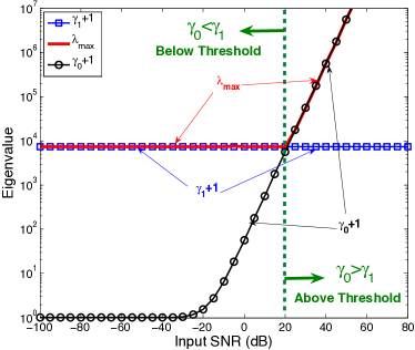
From Theorem 1 in Sec. III-A, we know that the empirical threshold SNRT0subscriptSNRT0\textsf{SNR}_{\textsf{T}0} is a key parameter for MPB. By the discussion in Sec. III-C, it is the intersection of the curves γ0+1subscript𝛾01\gamma_{0}\!\!+\!\!1 and γ1+1subscript𝛾11\gamma_{1}\!\!+\!\!1, as shown in Fig. 3(a). Therefore, we need to investigate these two parameters to gain deeper insight of SNRT0subscriptSNRT0\textsf{SNR}_{\textsf{T}0}.

IV-A General Results of γ0subscript𝛾0\gamma_{0} and γ1subscript𝛾1\gamma_{1}

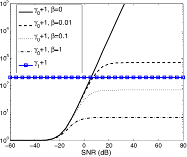
γ0subscript𝛾0\gamma_{0} has a simple expression of (36), from which we know that the parameter β𝛽\beta is critical. Fig. 3(b) shows the curve of γ0+1subscript𝛾01\gamma_{0}\!+\!1 with different β𝛽\beta. We see that, if β=0𝛽0\beta\!=\!0, i.e. 𝐇subscript𝐇\mathbf{H}_{\mathcal{I}} and 𝐡𝒮subscript𝐡𝒮\mathbf{h}_{\mathcal{S}} are orthogonal, then γ0=LSNRsubscript𝛾0𝐿SNR\gamma_{0}\!\!=\!\!L\textsf{SNR} is unbounded as SNR goes to infinity. Otherwise, there would be a limiting value of (Nβ)/β𝑁𝛽𝛽(N\!-\!\beta)/\beta so that γ0subscript𝛾0\gamma_{0} might never exceed γ1subscript𝛾1\gamma_{1} and SNRT0=+subscriptSNRT0\textsf{SNR}_{\textsf{T}0}\!\!=\!\!+\infty. Therefore, β=0𝛽0\beta\!\!=\!\!0 is the best choice for γ0subscript𝛾0\gamma_{0}.

Refer to caption
(a) The curves of γ0+1subscript𝛾01\gamma_{0}\!+\!1, γ1+1subscript𝛾11\gamma_{1}\!\!+\!\!1 and λmaxsubscript𝜆max\lambda_{\mathrm{max}} vs. SNR. (β=0𝛽0\beta=0)
Refer to caption
(b) γ0+1subscript𝛾01\gamma_{0}\!+\!1 against SNR with different β𝛽\beta.
Figure 3: The curve of γ0+1subscript𝛾01\gamma_{0}+1 and γ1+1subscript𝛾11\gamma_{1}+1 against SNR. The intersection of them is the empirical threshold SNRT0subscriptSNRT0\textsf{SNR}_{\textsf{T}0}.

γ1subscript𝛾1\gamma_{1} is another critical parameter that determines SNRT0subscriptSNRT0\textsf{SNR}_{\textsf{T}0}. Fig. 3 shows that, as γ1subscript𝛾1\gamma_{1} increases, its intersection with γ0subscript𝛾0\gamma_{0} moves rightward and SNRT0subscriptSNRT0\textsf{SNR}_{\textsf{T}0} increases. Therefore, knowing how to control γ1subscript𝛾1\gamma_{1} is important in designing MPB. By Lemma 5, γ1subscript𝛾1\gamma_{1} is the largest nonzero generalized eigenvalue of (𝐐𝒮𝐐,𝐐)subscript𝐐𝒮subscript𝐐subscript𝐐(\mathbf{Q}_{\mathcal{S}}\!-\!\mathbf{Q}_{\mathcal{I}},\mathbf{Q}_{\mathcal{I}}). (It is zero if there are less than D𝐷D nonzero eigenvalues and all of them are negative.) To solve it directly, we need the roots of a polynomial eigen-equation of order L𝐿L, which has no general formula when L>4𝐿4L\!\!>\!\!4. Instead, we resort to matrix perturbation theory again to derive a bound for it. We first notice that the eigen-decomposition of (𝐐𝒮𝐐,𝐐)subscript𝐐𝒮subscript𝐐subscript𝐐(\mathbf{Q}_{\mathcal{S}}\!-\!\mathbf{Q}_{\mathcal{I}},\mathbf{Q}_{\mathcal{I}}) is equivalent to (𝐐𝒮,𝐐)subscript𝐐𝒮subscript𝐐(\mathbf{Q}_{\mathcal{S}},\mathbf{Q}_{\mathcal{I}}) and their eigenvalues only differ by one. By (6) and (7), the eigenvalue of (𝐐𝒮,𝐐)subscript𝐐𝒮subscript𝐐(\mathbf{Q}_{\mathcal{S}},\mathbf{Q}_{\mathcal{I}}) is further equivalent to that of (𝐘𝒮+𝐈,𝐘+𝐈)subscript𝐘𝒮𝐈subscript𝐘𝐈(\mathbf{Y}_{\mathcal{S}}\!+\!\mathbf{I},\mathbf{Y}_{\mathcal{I}}\!+\!\mathbf{I}), where

𝐘𝒮=1σ2𝐀I𝚽𝒮𝐀IH=INR𝐀I𝚽𝒮0𝐀IH,𝐘=1σ2𝐀I𝚽𝐀IH=INR𝐀I𝚽0𝐀IH.formulae-sequencesubscript𝐘𝒮1superscript𝜎2subscript𝐀𝐼subscript𝚽𝒮superscriptsubscript𝐀𝐼𝐻INRsubscript𝐀𝐼subscript𝚽subscript𝒮0superscriptsubscript𝐀𝐼𝐻subscript𝐘1superscript𝜎2subscript𝐀𝐼subscript𝚽superscriptsubscript𝐀𝐼𝐻INRsubscript𝐀𝐼subscript𝚽subscript0superscriptsubscript𝐀𝐼𝐻\displaystyle\mathbf{Y}_{\mathcal{S}}=\frac{1}{\sigma^{2}}\mathbf{A}_{I}\bm{\Phi}_{\mathcal{S}}\mathbf{A}_{I}^{H}=\textsf{INR}\cdot\mathbf{A}_{I}\bm{\Phi}_{\mathcal{S}_{0}}\mathbf{A}_{I}^{H},\qquad\mathbf{Y}_{\mathcal{I}}=\frac{1}{\sigma^{2}}\mathbf{A}_{I}\bm{\Phi}_{\mathcal{I}}\mathbf{A}_{I}^{H}=\textsf{INR}\cdot\mathbf{A}_{I}\bm{\Phi}_{\mathcal{I}_{0}}\mathbf{A}_{I}^{H}. (42)

We term (𝐘𝒮,𝐘)subscript𝐘𝒮subscript𝐘(\mathbf{Y}_{\mathcal{S}},\mathbf{Y}_{\mathcal{I}}) as noise free pair, since it can be viewed as the covariance matrix pair of MPB without noise. Our strategy here is to view (𝐘𝒮+𝐈,𝐘+𝐈)subscript𝐘𝒮𝐈subscript𝐘𝐈(\mathbf{Y}_{\mathcal{S}}\!+\!\mathbf{I},\mathbf{Y}_{\mathcal{I}}\!+\!\mathbf{I}) as a perturbed version of (𝐘𝒮,𝐘)subscript𝐘𝒮subscript𝐘(\mathbf{Y}_{\mathcal{S}},\mathbf{Y}_{\mathcal{I}}) and apply the results in matrix perturbation theory to derive a bound for γ1+1subscript𝛾11\gamma_{1}\!\!+\!\!1. Before we proceed on, we cite a more general definition of the generalized eigenvalue of a matrix pair[32].

Definition 2 (Generalized eigenvalue)

The generalized eigenvalue of a matrix pair (𝐀,𝐁)𝐀𝐁\left(\mathbf{A},\mathbf{B}\right) is a one dimensional space, denoted as ν,μ{τ[νμ]:τ}𝜈𝜇conditional-set𝜏delimited-[]𝜈𝜇𝜏\langle\nu,\mu\rangle\triangleq\left\{\tau\cdot[\nu\;\mu]:\tau\in\mathbb{C}\right\}, where [νμ]delimited-[]𝜈𝜇[\nu\;\mu] is a 1×2121\times 2 vector satisfying

μ𝐀𝐱=ν𝐁𝐱,𝜇𝐀𝐱𝜈𝐁𝐱\displaystyle\mu\cdot\mathbf{A}\mathbf{x}=\nu\cdot\mathbf{B}\mathbf{x},

with 𝐱𝐱\mathbf{x} being its eigenvector. If 𝐁𝐁\mathbf{B} is nonsingular, then λ=ν/μ𝜆𝜈𝜇\lambda\!\!=\!\!\nu/\mu becomes the conventional definition.

Comparing to the conventional definition of generalized eigenvalues, this one includes the special case of 𝐁𝐁\mathbf{B} being singular so that μ=0𝜇0\mu\!\!=\!\!0 and ν0𝜈0\nu\!\!\neq\!\!0, namely, λ=+𝜆\lambda\!\!=\!\!+\infty. We will see its importance later. Besides, we also need the following definition and lemma from [32, pp.315–316].

Definition 3 (Definite pair)

If a matrix pair (𝐀,𝐁)𝐀𝐁(\mathbf{A},\mathbf{B}) consists of two Hermitian matrices and

C(𝐀,𝐁)min𝐱=1(𝐱H𝐀𝐱)2+(𝐱H𝐁𝐱)2>0,𝐶𝐀𝐁subscriptnorm𝐱1superscriptsuperscript𝐱𝐻𝐀𝐱2superscriptsuperscript𝐱𝐻𝐁𝐱20\displaystyle C(\mathbf{A},\mathbf{B})\triangleq\min_{\|\mathbf{x}\|=1}\sqrt{\left(\mathbf{x}^{H}\mathbf{A}\mathbf{x}\right)^{2}+\left(\mathbf{x}^{H}\mathbf{B}\mathbf{x}\right)^{2}}>0,

then (𝐀,𝐁)𝐀𝐁(\mathbf{A},\mathbf{B}) is called definite pair, and C(𝐀,𝐁)𝐶𝐀𝐁C(\mathbf{A},\mathbf{B}) is its Crawford number.

Theorem 2 (Weyl-Lidskii type)

Assume (𝐀,𝐁)𝐀𝐁\left(\mathbf{A},\mathbf{B}\right) is a definite pair and (𝐀+𝐄,𝐁+𝐅)𝐀𝐄𝐁𝐅\left(\mathbf{A}\!+\!\mathbf{E},\mathbf{B}\!+\!\mathbf{F}\right) is its perturbed version. Let αi,βisubscript𝛼𝑖subscript𝛽𝑖\langle\alpha_{i},\beta_{i}\rangle and α~i,β~isubscript~𝛼𝑖subscript~𝛽𝑖\langle\widetilde{\alpha}_{i},\widetilde{\beta}_{i}\rangle, (i=1,,n𝑖1𝑛i\!\!=\!\!1,\ldots,n), be their ordered generalized eigenvalues, respectively. If

𝐄S2+𝐅S2<C(𝐀,𝐁),superscriptsubscriptnorm𝐄𝑆2superscriptsubscriptnorm𝐅𝑆2𝐶𝐀𝐁\displaystyle{\sqrt{\|\mathbf{E}\|_{S}^{2}+\|\mathbf{F}\|_{S}^{2}}}<{C(\mathbf{A},\mathbf{B})}, (43)

where S\|\cdot\|_{S} denotes spectral norm of a matrix, then (𝐀~,𝐁~)~𝐀~𝐁(\widetilde{\mathbf{A}},\widetilde{\mathbf{B}}) is a definite pair, and

|α1β~2β1α~2||α1|2+|β1|2|α~2|2+|β~2|2𝐄S2+𝐅S2C(𝐀,𝐁),subscript𝛼1subscript~𝛽2subscript𝛽1subscript~𝛼2superscriptsubscript𝛼12superscriptsubscript𝛽12superscriptsubscript~𝛼22superscriptsubscript~𝛽22superscriptsubscriptnorm𝐄𝑆2superscriptsubscriptnorm𝐅𝑆2𝐶𝐀𝐁\displaystyle\frac{|\alpha_{1}\widetilde{\beta}_{2}-\beta_{1}\widetilde{\alpha}_{2}|}{\sqrt{|\alpha_{1}|^{2}+|\beta_{1}|^{2}}\sqrt{|\widetilde{\alpha}_{2}|^{2}+|\widetilde{\beta}_{2}|^{2}}}\leq\frac{\sqrt{\|\mathbf{E}\|_{S}^{2}+\|\mathbf{F}\|_{S}^{2}}}{C(\mathbf{A},\mathbf{B})},

We want to apply Theorem 2 to (𝐘𝒮+𝐈,𝐘+𝐈)subscript𝐘𝒮𝐈subscript𝐘𝐈(\mathbf{Y}_{\mathcal{S}}\!+\!\mathbf{I},\mathbf{Y}_{\mathcal{I}}\!+\!\mathbf{I}) and (𝐘𝒮,𝐘)subscript𝐘𝒮subscript𝐘(\mathbf{Y}_{\mathcal{S}},\mathbf{Y}_{\mathcal{I}}) to derive a bound for its eigenvalues. However, (𝐘𝒮,𝐘)subscript𝐘𝒮subscript𝐘(\mathbf{Y}_{\mathcal{S}},\mathbf{Y}_{\mathcal{I}}) is not a definite pair, for the null spaces of 𝐘𝒮subscript𝐘𝒮\mathbf{Y}_{\mathcal{S}} and 𝐘subscript𝐘\mathbf{Y}_{\mathcal{I}} may have nontrivial interset (larger than {0}0\{0\}). Therefore, we need to transform (𝐘𝒮,𝐘)subscript𝐘𝒮subscript𝐘(\mathbf{Y}_{\mathcal{S}},\mathbf{Y}_{\mathcal{I}}) into a definite pair. Let 𝒩𝒮subscript𝒩𝒮\mathcal{N}_{\mathcal{S}} and 𝒩subscript𝒩\mathcal{N}_{\mathcal{I}} be the null spaces of 𝐘𝒮subscript𝐘𝒮\mathbf{Y}_{\mathcal{S}} and 𝐘subscript𝐘\mathbf{Y}_{\mathcal{I}}, respectively, and 𝒩0𝒩𝒮𝒩subscript𝒩0subscript𝒩𝒮subscript𝒩\mathcal{N}_{0}\!\triangleq\!\mathcal{N}_{\mathcal{S}}\bigcap\mathcal{N}_{\mathcal{I}}. Let 𝐄0subscript𝐄0\mathbf{E}_{0} be a matrix whose columns are the orthonormal basis of 𝒩0superscriptsubscript𝒩0perpendicular-to\mathcal{N}_{0}^{\perp}, with 𝐄0H𝐄0=𝐈superscriptsubscript𝐄0𝐻subscript𝐄0𝐈\mathbf{E}_{0}^{H}\mathbf{E}_{0}=\mathbf{I}. Then, by the determinant identity in (31), (𝐘𝒮+𝐈,𝐘+𝐈)subscript𝐘𝒮𝐈subscript𝐘𝐈\left(\mathbf{Y}_{\mathcal{S}}\!+\!\mathbf{I},\mathbf{Y}_{\mathcal{I}}\!+\!\mathbf{I}\right) has the same generalized eigenvalues as (𝐄0H𝐘𝒮𝐄0+𝐈,𝐄0H𝐘𝐄0+𝐈)superscriptsubscript𝐄0𝐻subscript𝐘𝒮subscript𝐄0𝐈superscriptsubscript𝐄0𝐻subscript𝐘subscript𝐄0𝐈(\mathbf{E}_{0}^{H}\mathbf{Y}_{\mathcal{S}}\mathbf{E}_{0}\!+\!\mathbf{I},\mathbf{E}_{0}^{H}\mathbf{Y}_{\mathcal{I}}\mathbf{E}_{0}\!+\!\mathbf{I}), except for the multiplicity of ones. Similarly, (𝐄0H𝐘𝒮𝐄0,𝐄0H𝐘𝐄0)superscriptsubscript𝐄0𝐻subscript𝐘𝒮subscript𝐄0superscriptsubscript𝐄0𝐻subscript𝐘subscript𝐄0(\mathbf{E}_{0}^{H}\mathbf{Y}_{\mathcal{S}}\mathbf{E}_{0},\mathbf{E}_{0}^{H}\mathbf{Y}_{\mathcal{I}}\mathbf{E}_{0}) has the same eigenvalue as (𝐘𝒮,𝐘)subscript𝐘𝒮subscript𝐘(\mathbf{Y}_{\mathcal{S}},\mathbf{Y}_{\mathcal{I}}) does except for the multiplicity of zero. Therefore, instead, we can apply Theorem 2 to (𝐄0H𝐘𝒮𝐄0,𝐄0H𝐘𝐄0)superscriptsubscript𝐄0𝐻subscript𝐘𝒮subscript𝐄0superscriptsubscript𝐄0𝐻subscript𝐘subscript𝐄0(\mathbf{E}_{0}^{H}\mathbf{Y}_{\mathcal{S}}\mathbf{E}_{0},\mathbf{E}_{0}^{H}\mathbf{Y}_{\mathcal{I}}\mathbf{E}_{0}) and (𝐄0H𝐘𝒮𝐄0+𝐈,𝐄0H𝐘𝒮𝐄0+𝐈)superscriptsubscript𝐄0𝐻subscript𝐘𝒮subscript𝐄0𝐈superscriptsubscript𝐄0𝐻subscript𝐘𝒮subscript𝐄0𝐈(\mathbf{E}_{0}^{H}\mathbf{Y}_{\mathcal{S}}\mathbf{E}_{0}\!+\!\mathbf{I},\mathbf{E}_{0}^{H}\mathbf{Y}_{\mathcal{S}}\mathbf{E}_{0}\!+\!\mathbf{I}) to derive the bound. The Crawford number of (𝐄0H𝐘𝒮𝐄0,𝐄0H𝐘𝐄0)superscriptsubscript𝐄0𝐻subscript𝐘𝒮subscript𝐄0superscriptsubscript𝐄0𝐻subscript𝐘subscript𝐄0(\mathbf{E}_{0}^{H}\mathbf{Y}_{\mathcal{S}}\mathbf{E}_{0},\mathbf{E}_{0}^{H}\mathbf{Y}_{\mathcal{I}}\mathbf{E}_{0}) is

CYsubscript𝐶𝑌\displaystyle C_{Y} =min𝐰𝒩0,𝐰=1(𝐰H𝐘𝒮𝐰)2+(𝐰H𝐘𝐰)2>0,absentsubscriptformulae-sequence𝐰superscriptsubscript𝒩0perpendicular-tonorm𝐰1superscriptsuperscript𝐰𝐻subscript𝐘𝒮𝐰2superscriptsuperscript𝐰𝐻subscript𝐘𝐰20\displaystyle=\min_{\begin{subarray}{c}\mathbf{w}\in\mathcal{N}_{0}^{\perp},\;\|\mathbf{w}\|=1\end{subarray}}\sqrt{\left(\mathbf{w}^{H}\mathbf{Y}_{\mathcal{S}}\mathbf{w}\right)^{2}\!\!+\!\!\left(\mathbf{w}^{H}\mathbf{Y}_{\mathcal{I}}\mathbf{w}\right)^{2}}>0, (44)

which means (𝐄0H𝐘𝒮𝐄0,𝐄0H𝐘𝐄0)superscriptsubscript𝐄0𝐻subscript𝐘𝒮subscript𝐄0superscriptsubscript𝐄0𝐻subscript𝐘subscript𝐄0(\mathbf{E}_{0}^{H}\mathbf{Y}_{\mathcal{S}}\mathbf{E}_{0},\mathbf{E}_{0}^{H}\mathbf{Y}_{\mathcal{I}}\mathbf{E}_{0}) is a positive pair. Before applying Theorem 2, we first analyze the dependency of CYsubscript𝐶𝑌C_{Y} on the interference power. Substituting (42) into (44), we have CY=INRCY0subscript𝐶𝑌INRsubscript𝐶subscript𝑌0C_{Y}\!=\!\textsf{INR}\cdot C_{Y_{0}}, where

CY0subscript𝐶subscript𝑌0\displaystyle C_{Y_{0}} =min𝐰𝒩0,𝐰=1(𝐰H𝐀I𝚽𝒮0𝐀IH𝐰)2+(𝐰H𝐀I𝚽0𝐀IH𝐰)2.absentsubscriptformulae-sequence𝐰superscriptsubscript𝒩0perpendicular-tonorm𝐰1superscriptsuperscript𝐰𝐻subscript𝐀𝐼subscript𝚽subscript𝒮0superscriptsubscript𝐀𝐼𝐻𝐰2superscriptsuperscript𝐰𝐻subscript𝐀𝐼subscript𝚽subscript0superscriptsubscript𝐀𝐼𝐻𝐰2\displaystyle=\min_{{\mathbf{w}\in\mathcal{N}_{0}^{\perp},\;\|\mathbf{w}\|=1}}\sqrt{\left(\mathbf{w}^{H}\mathbf{A}_{I}\bm{\Phi}_{\mathcal{S}_{0}}\mathbf{A}_{I}^{H}\mathbf{w}\right)^{2}\!\!+\!\!\left(\mathbf{w}^{H}\mathbf{A}_{I}\bm{\Phi}_{\mathcal{I}_{0}}\mathbf{A}_{I}^{H}\mathbf{w}\right)^{2}}.

Since 𝚽𝒮0subscript𝚽subscript𝒮0\bm{\Phi}_{\mathcal{S}_{0}} and 𝚽0subscript𝚽subscript0\bm{\Phi}_{\mathcal{I}_{0}} are independent of INR (c.f. Sec. II-B), CY0subscript𝐶subscript𝑌0C_{Y_{0}} is also independent of INR. Therefore, CYsubscript𝐶𝑌C_{Y} is proportional to INR. Now, we are ready to use Theorem 2, and we only consider the case of INR being large. Let ν0,μ0subscript𝜈0subscript𝜇0\langle\nu_{0},\mu_{0}\rangle and ν,μ𝜈𝜇\langle\nu,\mu\rangle be the corresponding generalized eigenvalues of (𝐄0H𝐘𝒮𝐄0,𝐄0H𝐘𝐄0)superscriptsubscript𝐄0𝐻subscript𝐘𝒮subscript𝐄0superscriptsubscript𝐄0𝐻subscript𝐘subscript𝐄0(\mathbf{E}_{0}^{H}\mathbf{Y}_{\mathcal{S}}\mathbf{E}_{0},\mathbf{E}_{0}^{H}\mathbf{Y}_{\mathcal{I}}\mathbf{E}_{0}) and (𝐄0H𝐘𝒮𝐄0+𝐈,𝐄0H𝐘𝐄0+𝐈)superscriptsubscript𝐄0𝐻subscript𝐘𝒮subscript𝐄0𝐈superscriptsubscript𝐄0𝐻subscript𝐘subscript𝐄0𝐈(\mathbf{E}_{0}^{H}\mathbf{Y}_{\mathcal{S}}\mathbf{E}_{0}\!+\!\mathbf{I},\mathbf{E}_{0}^{H}\mathbf{Y}_{\mathcal{I}}\mathbf{E}_{0}\!+\!\mathbf{I}), respectively. Then, for large INR, (43) is satisfied and

|νμ0μν0||ν|2+|μ|2|ν0|2+|μ0|2<2CY01INR.𝜈subscript𝜇0𝜇subscript𝜈0superscript𝜈2superscript𝜇2superscriptsubscript𝜈02superscriptsubscript𝜇022subscript𝐶subscript𝑌01INR\displaystyle\frac{|\nu\mu_{0}-\mu\nu_{0}|}{\sqrt{|\nu|^{2}\!\!+\!\!|\mu|^{2}}\!\sqrt{|\nu_{0}|^{2}\!\!+\!\!|\mu_{0}|^{2}}}\!\!<\!\!\frac{\sqrt{2}}{C_{Y_{0}}}\cdot\frac{1}{\textsf{INR}}. (45)

We now derive the bound for γ1+1subscript𝛾11\gamma_{1}\!+\!1 in two separate cases.

IV-A1 𝒩𝒩𝒮not-subset-of-nor-equalssubscript𝒩subscript𝒩𝒮\mathcal{N}_{\mathcal{I}}\nsubseteq\mathcal{N}_{\mathcal{S}}

There is a nonzero 𝐰0subscript𝐰0\mathbf{w}_{0} such that 𝐘𝒮𝐰0𝟎subscript𝐘𝒮subscript𝐰00\mathbf{Y}_{\mathcal{S}}\mathbf{w}_{0}\!\neq\!\mathbf{0} and 𝐘𝐰0=𝟎subscript𝐘subscript𝐰00\mathbf{Y}_{\mathcal{I}}\mathbf{w}_{0}\!=\!\mathbf{0}. By Definition 2, ν0,0subscript𝜈00\langle\nu_{0},0\rangle (ν00for-allsubscript𝜈00\forall\nu_{0}\!\neq\!0) is a generalized eigenvalue of (𝐘𝒮,𝐘)subscript𝐘𝒮subscript𝐘(\mathbf{Y}_{\mathcal{S}},\mathbf{Y}_{\mathcal{I}}) and (𝐄0H𝐘𝒮𝐄0,𝐄0H𝐘𝐄0)superscriptsubscript𝐄0𝐻subscript𝐘𝒮subscript𝐄0superscriptsubscript𝐄0𝐻subscript𝐘subscript𝐄0(\mathbf{E}_{0}^{H}\mathbf{Y}_{\mathcal{S}}\mathbf{E}_{0},\mathbf{E}_{0}^{H}\mathbf{Y}_{\mathcal{I}}\mathbf{E}_{0}). This means the noise free pair (𝐘𝒮,𝐘)subscript𝐘𝒮subscript𝐘(\mathbf{Y}_{\mathcal{S}},\mathbf{Y}_{\mathcal{I}}) has an infinite generalized eigenvalue. As a result, (45) becomes

|μ||ν|2+|μ|2<2CY01INRλνμ>CY022INR21CY02INR.formulae-sequence𝜇superscript𝜈2superscript𝜇22subscript𝐶subscript𝑌01INR𝜆𝜈𝜇superscriptsubscript𝐶subscript𝑌022superscriptINR21subscript𝐶subscript𝑌02INR\displaystyle\frac{|\mu|}{\sqrt{|\nu|^{2}\!\!+\!\!|\mu|^{2}}}\!\!<\!\!\frac{\sqrt{2}}{C_{Y_{0}}}\cdot\frac{1}{\textsf{INR}}\quad\Leftrightarrow\quad\lambda\triangleq\frac{\nu}{\mu}>\sqrt{\frac{C_{Y_{0}}^{2}}{2}\textsf{INR}^{2}\!\!-\!\!1}\approx\frac{C_{Y_{0}}}{\sqrt{2}}\textsf{INR}.

This means (𝐄0H𝐘𝒮𝐄0+𝐈,𝐄0H𝐘𝒮𝐄0+𝐈)superscriptsubscript𝐄0𝐻subscript𝐘𝒮subscript𝐄0𝐈superscriptsubscript𝐄0𝐻subscript𝐘𝒮subscript𝐄0𝐈(\mathbf{E}_{0}^{H}\mathbf{Y}_{\mathcal{S}}\mathbf{E}_{0}\!+\!\mathbf{I},\mathbf{E}_{0}^{H}\mathbf{Y}_{\mathcal{S}}\mathbf{E}_{0}\!+\!\mathbf{I}) would always have an eigenvalue that satisfies the above inequality. Since (𝐐𝒮,𝐐)subscript𝐐𝒮subscript𝐐(\mathbf{Q}_{\mathcal{S}},\mathbf{Q}_{\mathcal{I}}) has the same eigenvalue except for the multiplicity of ones, γ1+1subscript𝛾11\gamma_{1}\!+\!1 satisfies

γ1+1>CY02INR,subscript𝛾11subscript𝐶subscript𝑌02INR\displaystyle\gamma_{1}+1>\frac{C_{Y_{0}}}{\sqrt{2}}\textsf{INR}, (46)

which gives a lower bound for γ1+1subscript𝛾11\gamma_{1}\!+\!1. We can see that it goes up unboundedly as INR increases. Hence, by (22) and (24), the threshold SNR also increases unboundedly with INR.

IV-A2 𝒩𝒩𝒮subscript𝒩subscript𝒩𝒮\mathcal{N}_{\mathcal{I}}\subseteq\mathcal{N}_{\mathcal{S}}

Then, 𝒩0=𝒩subscript𝒩0subscript𝒩\mathcal{N}_{0}\!=\!\mathcal{N}_{\mathcal{I}} and 𝐄0H𝐘𝐄0superscriptsubscript𝐄0𝐻subscript𝐘subscript𝐄0\mathbf{E}_{0}^{H}\mathbf{Y}_{\mathcal{I}}\mathbf{E}_{0} is nonsingular. As a result, all eigenvalues of (𝐄0H𝐘𝒮𝐄0,𝐄0H𝐘𝐄0)superscriptsubscript𝐄0𝐻subscript𝐘𝒮subscript𝐄0superscriptsubscript𝐄0𝐻subscript𝐘subscript𝐄0(\mathbf{E}_{0}^{H}\mathbf{Y}_{\mathcal{S}}\mathbf{E}_{0},\mathbf{E}_{0}^{H}\mathbf{Y}_{\mathcal{I}}\mathbf{E}_{0}) and (𝐘𝒮,𝐘)subscript𝐘𝒮subscript𝐘(\mathbf{Y}_{\mathcal{S}},\mathbf{Y}_{\mathcal{I}}) are bounded. When INR is large, (45) becomes

|λλ0|1+λ21+λ02<CY021INR|λλ0|<CY02(1+λ02)1INRformulae-sequence𝜆subscript𝜆01superscript𝜆21superscriptsubscript𝜆02subscript𝐶subscript𝑌021INR𝜆subscript𝜆0subscript𝐶subscript𝑌021superscriptsubscript𝜆021INR\displaystyle\frac{|\lambda-\lambda_{0}|}{\sqrt{1+\lambda^{2}}\sqrt{1+\lambda_{0}^{2}}}<\frac{C_{Y_{0}}}{\sqrt{2}}\cdot\frac{1}{\textsf{INR}}\quad\Longrightarrow\quad|\lambda-\lambda_{0}|<\frac{C_{Y_{0}}}{\sqrt{2}}(1+\lambda_{0}^{2})\cdot\frac{1}{\textsf{INR}}

where λ0=ν0/μ0subscript𝜆0subscript𝜈0subscript𝜇0\lambda_{0}\!=\!\nu_{0}/\mu_{0} is the largest eigenvalue of (𝐄0H𝐘𝒮𝐄0,𝐄0H𝐘𝒮𝐄0)superscriptsubscript𝐄0𝐻subscript𝐘𝒮subscript𝐄0superscriptsubscript𝐄0𝐻subscript𝐘𝒮subscript𝐄0(\mathbf{E}_{0}^{H}\mathbf{Y}_{\mathcal{S}}\mathbf{E}_{0},\mathbf{E}_{0}^{H}\mathbf{Y}_{\mathcal{S}}\mathbf{E}_{0}) and we used λλ0𝜆subscript𝜆0\lambda\!\approx\lambda_{0} in the second inequality. Since (𝐐𝒮,𝐐)subscript𝐐𝒮subscript𝐐(\mathbf{Q}_{\mathcal{S}},\mathbf{Q}_{\mathcal{I}}) has the same eigenvalue as (𝐄0H𝐘𝒮𝐄0+𝐈,𝐄0H𝐘𝒮𝐄0+𝐈)superscriptsubscript𝐄0𝐻subscript𝐘𝒮subscript𝐄0𝐈superscriptsubscript𝐄0𝐻subscript𝐘𝒮subscript𝐄0𝐈(\mathbf{E}_{0}^{H}\mathbf{Y}_{\mathcal{S}}\mathbf{E}_{0}\!+\!\mathbf{I},\mathbf{E}_{0}^{H}\mathbf{Y}_{\mathcal{S}}\mathbf{E}_{0}\!+\!\mathbf{I}) except for the multiplicity of ones, γ1+1subscript𝛾11\gamma_{1}+1 is bounded around the largest eigenvalue of (𝐘𝒮,𝐘)subscript𝐘𝒮subscript𝐘(\mathbf{Y}_{\mathcal{S}},\mathbf{Y}_{\mathcal{I}}) or one. Furthermore, from (42), we know that λ0subscript𝜆0\lambda_{0} is independent of INR. Therefore, as all eigenvalues of noise free pair is finite, γ1+1subscript𝛾11\gamma_{1}\!+\!1 is bounded and independent of INR.

IV-B Two Typical Scenarios of γ1subscript𝛾1\gamma_{1}

From the previous part, we know that whether the threshold of MPB is unbounded is determined by the existence of infinite eigenvalue of the noise free pair. Now, we discuss two typical classes of interferences. In the first case, all eigenvalues are finite, and in the second case, there may be infinite eigenvalues.

IV-B1 Directional White Noise

By uncorrelated directional white noise, we mean an interference that arrives from a specific direction, with its samples in time domain being uncorrelated. This means the entries of 𝐒I(k)subscript𝐒𝐼𝑘\mathbf{S}_{I}(k) are independent identically distributed random variables with zero mean and unit variance. (In section II-A, we have already normalized the interference power in 𝐬i(k)subscript𝐬𝑖𝑘\mathbf{s}_{i}(k).) Then, by (8), we can immediately have 𝚽𝒮0=𝚽0subscript𝚽subscript𝒮0subscript𝚽subscript0\bm{\Phi}_{\mathcal{S}_{0}}\!=\!\bm{\Phi}_{\mathcal{I}_{0}}, and all the eigenvalue of the noise free pair (𝐘𝒮,𝐘)subscript𝐘𝒮subscript𝐘(\mathbf{Y}_{\mathcal{S}},\mathbf{Y}_{\mathcal{I}}) are ones. Thus, in this case, γ1+1subscript𝛾11\gamma_{1}\!+\!1 is bounded and is independent of INR. In fact, we can further have 𝐐𝒮=𝐐subscript𝐐𝒮subscript𝐐\mathbf{Q}_{\mathcal{S}}\!=\!\mathbf{Q}_{\mathcal{I}} according to (6) and (7). Therefore, γ1=0subscript𝛾10\gamma_{1}\!=\!0, SNRT0=0subscriptSNRT00\textsf{SNR}_{\textsf{T}0}\!=\!0 and G(SNR)=1GSNR1\textsf{G}(\textsf{SNR})\!=\!1.

IV-B2 Directional Periodical Interference

If an interference has periodical structure in time domain and arrives from certain direction, then we term it as directional periodical interference. By periodical, we mean the interfer is periodic with respect to the projection basis, i.e.

𝐇H𝐒I(k)=ejϕk𝐇H𝐒I,𝐡𝒮H𝐒I(k)=ejϕk𝐡𝒮H𝐒I.formulae-sequencesuperscriptsubscript𝐇𝐻subscript𝐒𝐼𝑘superscript𝑒𝑗subscriptitalic-ϕ𝑘superscriptsubscript𝐇𝐻subscript𝐒𝐼superscriptsubscript𝐡𝒮𝐻subscript𝐒𝐼𝑘superscript𝑒𝑗superscriptsubscriptitalic-ϕ𝑘superscriptsubscript𝐡𝒮𝐻subscript𝐒𝐼\displaystyle\mathbf{H}_{\mathcal{I}}^{H}\mathbf{S}_{I}(k)=e^{j\phi_{k}}\mathbf{H}_{\mathcal{I}}^{H}\mathbf{S}_{I},\qquad\mathbf{h}_{\mathcal{S}}^{H}\mathbf{S}_{I}(k)=e^{j\phi_{k}^{\prime}}\mathbf{h}_{\mathcal{S}}^{H}\mathbf{S}_{I}. (47)

A stronger condition would be 𝐒I(k)=𝐒Isubscript𝐒𝐼𝑘subscript𝐒𝐼\mathbf{S}_{I}(k)\!=\!\mathbf{S}_{I}. However, (47) is good enough for our analysis. Now, we will discuss the existence of infinite generalized eigenvalue in the noise free pair (𝐘𝒮,𝐘)subscript𝐘𝒮subscript𝐘(\mathbf{Y}_{\mathcal{S}},\mathbf{Y}_{\mathcal{I}}). To do this, we need to consider the relationship between their null spaces.

In practice, 𝐑𝒮subscript𝐑𝒮\mathbf{R}_{\mathcal{S}} and 𝐑subscript𝐑\mathbf{R}_{\mathcal{I}} are estimated from sample average. Therefore, replacing the expectation in (8) by sample average and using (47), we can get

𝚽𝒮0=𝛀I1/2𝐒IT𝐡𝒮𝐡𝒮T𝐒I𝛀I1/2,𝚽0=1r𝛀I1/2𝐒IT𝐇𝐇T𝐒I𝛀I1/2.formulae-sequencesubscript𝚽subscript𝒮0superscriptsubscript𝛀𝐼12superscriptsubscript𝐒𝐼𝑇superscriptsubscript𝐡𝒮superscriptsubscript𝐡𝒮𝑇superscriptsubscript𝐒𝐼superscriptsubscript𝛀𝐼12subscript𝚽subscript01subscript𝑟superscriptsubscript𝛀𝐼12superscriptsubscript𝐒𝐼𝑇superscriptsubscript𝐇superscriptsubscript𝐇𝑇superscriptsubscript𝐒𝐼superscriptsubscript𝛀𝐼12\displaystyle\bm{\Phi}_{\mathcal{S}_{0}}=\bm{\Omega}_{I}^{1/2}\mathbf{S}_{I}^{T}\mathbf{h}_{\mathcal{S}}^{\ast}\mathbf{h}_{\mathcal{S}}^{T}\mathbf{S}_{I}^{\ast}\bm{\Omega}_{I}^{1/2},\qquad\bm{\Phi}_{\mathcal{I}_{0}}=\frac{1}{r_{\mathcal{I}}}\bm{\Omega}_{I}^{1/2}\mathbf{S}_{I}^{T}\mathbf{H}_{\mathcal{I}}^{\ast}\mathbf{H}_{\mathcal{I}}^{T}\mathbf{S}_{I}^{\ast}\bm{\Omega}_{I}^{1/2}.

Let 𝚷𝐒I𝛀I1/2𝐀IT𝚷subscript𝐒𝐼superscriptsubscript𝛀𝐼12superscriptsubscript𝐀𝐼𝑇\bm{\Pi}\!\triangleq\!\mathbf{S}_{I}\bm{\Omega}_{I}^{1/2}\mathbf{A}_{I}^{T}. Then, by (42), 𝐘𝒮subscript𝐘𝒮\mathbf{Y}_{\mathcal{S}} and 𝐘subscript𝐘\mathbf{Y}_{\mathcal{I}} in this case can be expressed as

𝐘𝒮=INR(𝚷H𝐡𝒮𝐡𝒮H𝚷),𝐘=INR1r(𝚷H𝐇𝐇H𝚷).formulae-sequencesubscript𝐘𝒮INRsuperscriptsuperscript𝚷𝐻subscript𝐡𝒮superscriptsubscript𝐡𝒮𝐻𝚷subscript𝐘INR1subscript𝑟superscriptsuperscript𝚷𝐻subscript𝐇superscriptsubscript𝐇𝐻𝚷\displaystyle\mathbf{Y}_{\mathcal{S}}=\textsf{INR}\cdot\left(\bm{\Pi}^{H}\mathbf{h}_{\mathcal{S}}\mathbf{h}_{\mathcal{S}}^{H}\bm{\Pi}\right)^{\ast},\qquad\mathbf{Y}_{\mathcal{I}}=\textsf{INR}\cdot\frac{1}{r_{\mathcal{I}}}\left(\bm{\Pi}^{H}\mathbf{H}_{\mathcal{I}}\mathbf{H}_{\mathcal{I}}^{H}\bm{\Pi}\right)^{\ast}. (48)

Therefore, the noise free pair (𝐘𝒮,𝐘)subscript𝐘𝒮subscript𝐘(\mathbf{Y}_{\mathcal{S}},\mathbf{Y}_{\mathcal{I}}) has the same eigenvalue as (𝚷H𝐡𝒮𝐡𝒮H𝚷,1r𝚷H𝐇𝐇H𝚷)superscript𝚷𝐻subscript𝐡𝒮superscriptsubscript𝐡𝒮𝐻𝚷1subscript𝑟superscript𝚷𝐻subscript𝐇superscriptsubscript𝐇𝐻𝚷(\bm{\Pi}^{H}\mathbf{h}_{\mathcal{S}}\mathbf{h}_{\mathcal{S}}^{H}\bm{\Pi},\frac{1}{r_{\mathcal{I}}}\bm{\Pi}^{H}\mathbf{H}_{\mathcal{I}}\mathbf{H}_{\mathcal{I}}^{H}\bm{\Pi}) does, and we only have to check the null spaces of later matrix pair. Let 𝒱I(𝚷)subscript𝒱𝐼𝚷\mathcal{V}_{I}\!\triangleq\!\mathcal{R}(\bm{\Pi}) be the range space of 𝚷𝚷\bm{\Pi}. By definition, it is also the range space of 𝐒Isubscript𝐒𝐼\mathbf{S}_{I}, namely the space spanned by all interference waveforms in one period. Then, we can express the null spaces of 𝚷H𝐡𝒮𝐡𝒮H𝚷superscript𝚷𝐻subscript𝐡𝒮superscriptsubscript𝐡𝒮𝐻𝚷\bm{\Pi}^{H}\mathbf{h}_{\mathcal{S}}\mathbf{h}_{\mathcal{S}}^{H}\bm{\Pi} and 𝚷H𝐇𝐇H𝚷superscript𝚷𝐻subscript𝐇superscriptsubscript𝐇𝐻𝚷\bm{\Pi}^{H}\mathbf{H}_{\mathcal{I}}\mathbf{H}_{\mathcal{I}}^{H}\bm{\Pi} as

𝒩𝒮𝒩(𝚷H𝐡𝒮𝐡𝒮H𝚷)={𝚷𝐱:𝐱𝒮𝒱I}𝒩(𝚷)superscriptsubscript𝒩𝒮𝒩superscript𝚷𝐻subscript𝐡𝒮superscriptsubscript𝐡𝒮𝐻𝚷direct-sumconditional-setsuperscript𝚷𝐱𝐱superscript𝒮perpendicular-tosubscript𝒱𝐼𝒩𝚷\displaystyle\mathcal{N}_{\mathcal{S}}^{\prime}\triangleq\mathcal{N}\left(\bm{\Pi}^{H}\mathbf{h}_{\mathcal{S}}\mathbf{h}_{\mathcal{S}}^{H}\bm{\Pi}\right)=\left\{\bm{\Pi}^{\dagger}\mathbf{x}:\;\mathbf{x}\in\mathcal{S}^{\perp}\cap\mathcal{V}_{I}\right\}\oplus\mathcal{N}(\bm{\Pi})
𝒩𝒩(𝚷H𝐇𝐇H𝚷)={𝚷𝐱:𝐱𝒱I}𝒩(𝚷),superscriptsubscript𝒩𝒩superscript𝚷𝐻subscript𝐇superscriptsubscript𝐇𝐻𝚷direct-sumconditional-setsuperscript𝚷𝐱𝐱superscriptperpendicular-tosubscript𝒱𝐼𝒩𝚷\displaystyle\mathcal{N}_{\mathcal{I}}^{\prime}\triangleq\mathcal{N}\left(\bm{\Pi}^{H}\mathbf{H}_{\mathcal{I}}\mathbf{H}_{\mathcal{I}}^{H}\bm{\Pi}\right)=\left\{\bm{\Pi}^{\dagger}\mathbf{x}:\;\mathbf{x}\in\mathcal{I}^{\perp}\cap\mathcal{V}_{I}\right\}\oplus\mathcal{N}(\bm{\Pi}),

where 𝒮=(𝐡𝒮)𝒮subscript𝐡𝒮\mathcal{S}\!=\!\mathcal{R}(\mathbf{h}_{\mathcal{S}}), =(𝐇)subscript𝐇\mathcal{I}\!=\!\mathcal{R}(\mathbf{H}_{\mathcal{I}}) as defined in Sec. II-B, and \dagger denotes Moore-Penrose pseudoinverse [34]. To see the relationship between 𝒩𝒮superscriptsubscript𝒩𝒮\mathcal{N}_{\mathcal{S}}^{\prime} and 𝒩superscriptsubscript𝒩\mathcal{N}_{\mathcal{I}}^{\prime}, we only need to check the relationship between 𝒮𝒱Isuperscript𝒮perpendicular-tosubscript𝒱𝐼\mathcal{S}^{\perp}\cap\mathcal{V}_{I} and 𝒱Isuperscriptperpendicular-tosubscript𝒱𝐼\mathcal{I}^{\perp}\cap\mathcal{V}_{I} which can be expressed as

𝒮𝒱I={𝐱:𝐁𝒮H𝐱=𝟎},𝒱I={𝐱:𝐁H𝐱=𝟎},formulae-sequencesuperscript𝒮perpendicular-tosubscript𝒱𝐼conditional-set𝐱superscriptsubscript𝐁𝒮𝐻𝐱0superscriptperpendicular-tosubscript𝒱𝐼conditional-set𝐱superscriptsubscript𝐁𝐻𝐱0\displaystyle\mathcal{S}^{\perp}\cap\mathcal{V}_{I}=\{\mathbf{x}:\;\mathbf{B}_{\mathcal{S}}^{H}\mathbf{x}=\mathbf{0}\},\qquad\mathcal{I}^{\perp}\cap\mathcal{V}_{I}=\{\mathbf{x}:\;\mathbf{B}_{\mathcal{I}}^{H}\mathbf{x}=\mathbf{0}\}, (49)

where

𝐁[𝐇𝒱I𝐇],𝐁𝒮[𝐇𝒱I𝐡𝒮].formulae-sequencesubscript𝐁matrixsubscript𝐇superscriptsubscript𝒱𝐼perpendicular-tosubscript𝐇subscript𝐁𝒮matrixsubscript𝐇superscriptsubscript𝒱𝐼perpendicular-tosubscript𝐡𝒮\displaystyle\mathbf{B}_{\mathcal{I}}\triangleq\begin{bmatrix}\mathbf{H}_{\mathcal{V}_{I}^{\perp}}&\mathbf{H}_{\mathcal{I}}\\ \end{bmatrix},\qquad\mathbf{B}_{\mathcal{S}}\triangleq\begin{bmatrix}\mathbf{H}_{\mathcal{V}_{I}^{\perp}}&\mathbf{h}_{\mathcal{S}}\\ \end{bmatrix}.

with 𝐇𝒱Isubscript𝐇superscriptsubscript𝒱𝐼perpendicular-to\mathbf{H}_{\mathcal{V}_{I}^{\perp}} being the matrix whose columns are the orthonormal basis of 𝒱Isuperscriptsubscript𝒱𝐼perpendicular-to\mathcal{V}_{I}^{\perp}. Then, by (49), whether the eigenvalues of (𝐘𝒮,𝐘)subscript𝐘𝒮subscript𝐘(\mathbf{Y}_{\mathcal{S}},\mathbf{Y}_{\mathcal{I}}) are finite is equivalent to the validity of {𝐁}{𝐁𝒮}subscript𝐁𝒮subscript𝐁\mathcal{R}\{\mathbf{B}_{\mathcal{I}}\}\!\!\supseteq\!\!\mathcal{R}\{\mathbf{B}_{\mathcal{S}}\}. Define

𝐓𝐁[𝐈𝐇𝒱IH𝐇0𝐈],𝐓𝐁𝒮[𝐈𝐇𝒱IH𝐡𝒮0𝐈].formulae-sequencesubscript𝐓subscript𝐁matrix𝐈superscriptsubscript𝐇superscriptsubscript𝒱𝐼perpendicular-to𝐻subscript𝐇0𝐈subscript𝐓subscript𝐁𝒮matrix𝐈superscriptsubscript𝐇superscriptsubscript𝒱𝐼perpendicular-to𝐻subscript𝐡𝒮0𝐈\displaystyle\mathbf{T}_{\mathbf{B}_{\mathcal{I}}}\triangleq\begin{bmatrix}\mathbf{I}&-\mathbf{H}_{\mathcal{V}_{I}^{\perp}}^{H}\mathbf{H}_{\mathcal{I}}\\ 0&\mathbf{I}\end{bmatrix},\qquad\mathbf{T}_{\mathbf{B}_{\mathcal{S}}}\triangleq\begin{bmatrix}\mathbf{I}&-\mathbf{H}_{\mathcal{V}_{I}^{\perp}}^{H}\mathbf{h}_{\mathcal{S}}\\ 0&\mathbf{I}\end{bmatrix}.

Right-multiplying 𝐁subscript𝐁\mathbf{B}_{\mathcal{I}} and 𝐁𝒮subscript𝐁𝒮\mathbf{B}_{\mathcal{S}} by 𝐓𝐁subscript𝐓subscript𝐁\mathbf{T}_{\mathbf{B}_{\mathcal{I}}} and 𝐓𝐁𝒮subscript𝐓subscript𝐁𝒮\mathbf{T}_{\mathbf{B}_{\mathcal{S}}}, respectively, we can have

𝐁𝐓𝐁=[𝐇𝒱c𝐏𝒱I𝐇],𝐁𝒮𝐓𝐁𝒮=[𝐇𝒱c𝐏𝒱I𝐡𝒮],formulae-sequencesubscript𝐁subscript𝐓subscript𝐁matrixsubscript𝐇superscriptsubscript𝒱𝑐perpendicular-tosubscript𝐏subscript𝒱𝐼subscript𝐇subscript𝐁𝒮subscript𝐓subscript𝐁𝒮matrixsubscript𝐇superscriptsubscript𝒱𝑐perpendicular-tosubscript𝐏subscript𝒱𝐼subscript𝐡𝒮\displaystyle\mathbf{B}_{\mathcal{I}}\cdot\mathbf{T}_{\mathbf{B}_{\mathcal{I}}}=\begin{bmatrix}\mathbf{H}_{\mathcal{V}_{c}^{\perp}}&\mathbf{P}_{\mathcal{V}_{I}}\mathbf{H}_{\mathcal{I}}\end{bmatrix},\qquad\mathbf{B}_{\mathcal{S}}\cdot\mathbf{T}_{\mathbf{B}_{\mathcal{S}}}=\begin{bmatrix}\mathbf{H}_{\mathcal{V}_{c}^{\perp}}&\mathbf{P}_{\mathcal{V}_{I}}\mathbf{h}_{\mathcal{S}}\end{bmatrix},

where 𝐏𝒱I𝐇𝒱I𝐇𝒱IHsubscript𝐏subscript𝒱𝐼subscript𝐇subscript𝒱𝐼superscriptsubscript𝐇subscript𝒱𝐼𝐻\mathbf{P}_{\mathcal{V}_{I}}\!\triangleq\!\mathbf{H}_{\mathcal{V}_{I}}\mathbf{H}_{\mathcal{V}_{I}}^{H} is the projection matrix onto 𝒱Isubscript𝒱𝐼\mathcal{V}_{I}. Since 𝐓𝐁subscript𝐓subscript𝐁\mathbf{T}_{\mathbf{B}_{\mathcal{I}}} and 𝐓𝐁𝒮subscript𝐓subscript𝐁𝒮\mathbf{T}_{\mathbf{B}_{\mathcal{S}}} are nonsingular, the above two matrices have the same range spaces as 𝐁𝒮subscript𝐁𝒮\mathbf{B}_{\mathcal{S}} and 𝐁subscript𝐁\mathbf{B}_{\mathcal{I}} do, namely we can have

{𝐁}=𝒱I{𝐏𝒱I𝐇},{𝐁𝒮}=𝒱I{𝐏𝒱I𝐡𝒮}formulae-sequencesubscript𝐁direct-sumsuperscriptsubscript𝒱𝐼perpendicular-tosubscript𝐏subscript𝒱𝐼subscript𝐇subscript𝐁𝒮direct-sumsuperscriptsubscript𝒱𝐼perpendicular-tosubscript𝐏subscript𝒱𝐼subscript𝐡𝒮\displaystyle\mathcal{R}\{\mathbf{B}_{\mathcal{I}}\}=\mathcal{V}_{I}^{\perp}\oplus\mathcal{R}\{\mathbf{P}_{\mathcal{V}_{I}}\mathbf{H}_{\mathcal{I}}\},\qquad\mathcal{R}\{\mathbf{B}_{\mathcal{S}}\}=\mathcal{V}_{I}^{\perp}\oplus\mathcal{R}\{\mathbf{P}_{\mathcal{V}_{I}}\mathbf{h}_{\mathcal{S}}\}

Therefore, whether the generalized eigenvalues of the noise free pair are bounded is finally equivalent to whether

{𝐏𝒱I𝐇}{𝐏𝒱c𝐡𝒮}.subscript𝐏subscript𝒱𝑐subscript𝐡𝒮subscript𝐏subscript𝒱𝐼subscript𝐇\displaystyle\mathcal{R}\big{\{}\mathbf{P}_{\mathcal{V}_{I}}\mathbf{H}_{\mathcal{I}}\big{\}}\!\!\supseteq\!\!\mathcal{R}\big{\{}\mathbf{P}_{\mathcal{V}_{c}}\mathbf{h}_{\mathcal{S}}\big{\}}. (50)
Refer to caption
Figure 4: Geometrical interpretation of (50). 𝐡(1)superscriptsubscript𝐡1\mathbf{h}_{\mathcal{I}}^{(1)} and 𝐡(2)superscriptsubscript𝐡2\mathbf{h}_{\mathcal{I}}^{(2)} denote the columns of 𝐇subscript𝐇\mathbf{H}_{\mathcal{I}}. For one interference channel, 𝐇=𝐡subscript𝐇subscript𝐡\mathbf{H}_{\mathcal{I}}\!=\!\mathbf{h}_{\mathcal{I}}.

Fig. 4 shows the geometrical interpretation of (50). To see if γ1subscript𝛾1\gamma_{1} is bounded, we can project 𝐡𝒮subscript𝐡𝒮\mathbf{h}_{\mathcal{S}} and all the columns of 𝐇subscript𝐇\mathbf{H}_{\mathcal{I}} onto 𝒱Isubscript𝒱𝐼\mathcal{V}_{I}. If the former projection lies in the space spanned by the later ones, then γ1subscript𝛾1\gamma_{1} is bounded. Otherwise, there is an infinite eigenvalue in the noise free pair and γ1subscript𝛾1\gamma_{1} will increase unboundedly with INR. Since 𝐇subscript𝐇\mathbf{H}_{\mathcal{I}} of the Maximin scheme and PAPC scheme has only one column, this means the projections of 𝐡𝒮subscript𝐡𝒮\mathbf{h}_{\mathcal{S}} and 𝐇subscript𝐇\mathbf{H}_{\mathcal{I}} should be on the same line, which is hardly valid. Thus, these two approaches are sensitive to directional periodical interferences, as we will see in later simulation results. Furthermore, Fig. 4 also shows the case of multiple interference channels, i.e. the dimension of \mathcal{I} is larger than one, then γ1subscript𝛾1\gamma_{1} is more likely to be bounded. This issue is out of the scope of this paper and will be discussed in in [36].

V Simulation Results

In this section, we simulate various scenarios and compare them to our theoretical results. The matrix pair beamformers implemented include the Maximin algorithm and PAPC algorithm, which have many kinds of adaptive algorithms. However, we are only interested in their steady state performance. The reason for this is that, if the methods suffer from poor steady state performance, then it is meaningless to investigate their adaptive algorithms. Therefore, we directly calculate their weight vectors by performing generalized eigen-decompositions on the estimated matrix pairs. The interference signals encountered in the simulation include BPSK signal, tones, periodical noise and multiuser interference. The first one is the directional white noise and the others are directional periodical interferences.

In all cases, we consider a uniform linear array (ULA) with eight isotropic antennas (L=8𝐿8L=8) spaced half a wavelength apart. For each user, a 100100100 kbps DPSK signal is randomly generated and spreaded by a distinct 31-chip Gold sequence in each simulation trial. Then it is modulated onto a 111 GHz carrier to form a RF signal with bandwidth 3.13.13.1 MHz. In all the simulations, we assume the SOI arrives from 0superscript00^{\circ} and the interferers have equal power.

Fig. 5(a)–Fig. 5(d) show the operating curve G(SNR)GSNR\textsf{G}(\textsf{SNR}) of the Maximin and PAPC beamformers in the four scenarios. The simulated values are obtained by using the simulated data and the theoretical ones are computed by the piecewise function G(SNR)GSNR\textsf{G}(\textsf{SNR}) in (20). To eliminate the randomness caused by finite sample effects, K=106𝐾superscript106K=10^{6} symbols are simulated for each SNR and INR in every experiment.
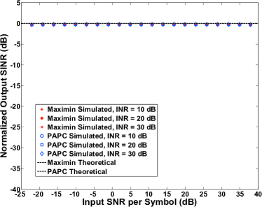
Refer to caption
(a) G(SNR)GSNR\textsf{G}(\textsf{SNR}) of Maximin and PAPC under BPSK jammers.
Refer to caption
(b) G(SNR)GSNR\textsf{G}(\textsf{SNR}) of Maximin and PAPC under periodical noise.
Refer to caption
(c) G(SNR)GSNR\textsf{G}(\textsf{SNR}) of Maximin and PAPC under tone jammers.
Refer to caption
(d) G(SNR)GSNR\textsf{G}(\textsf{SNR}) of Maximin and PAPC under multipath MAI.
Figure 5: Simulated and theoretical operating curve G(SNR)GSNR\textsf{G}(\textsf{SNR}) under different kinds of interference for Maximin and PAPC.

In Fig. 5(a), the interferers are three uncorrelated BPSK modulated signals, i.e. random sequences of ±1plus-or-minus1\pm 1. The rates of the interferers are all 3.1Mbps, which is the same as the chip rate of the SOI and covers its whole bandwidth. Therefore, they belong to the type of directional white noise. We can see that G(SNR)1GSNR1\textsf{G}(\textsf{SNR})\approx 1 and there is no threshold effect, which is consistent with the analysis in Section IV-B1.

Fig. 5(b)–Fig. 5(d) show the results for three types of directional periodical interferences: periodical noise, tones and multiple access interference (MAI) with multipath. In Fig. 5(b), we consider two periodical noises, which arrives from 30superscript3030^{\circ} and 40superscript40-40^{\circ}, respectively, and each of them is generated by repeating a segment of Gaussian white noise over times, with the repeating frequency being 100100100 kHz (same as that of SOI’s symbol rate). The frequency offsets of the tones with respect to the carrier in Fig. 5(c) are 100100100kHz, 300300-300kHz, 00Hz, 400400400kHz and 100100-100kHz, respectively, and their DOAs are 30superscript3030^{\circ}, 50superscript50-50^{\circ}, 20superscript20-20^{\circ}, 19superscript1919^{\circ} and 45superscript4545^{\circ}. In Fig. 5(d), there is one incident MAI signal with three-ray multipath delays of 333 chips, 555 chips and 444 chips arriving from 30superscript3030^{\circ}, 20superscript20-20^{\circ} and 50superscript50-50^{\circ}, respectively. We can see that the theoretical values of G(SNR)GSNR\textsf{G}(\textsf{SNR}) match with the simulated ones very well.

To verify the validity of the approximation given by Lemma 4, in Fig. 6(a) and Fig. 6(b), we also show the curves of γ0+1subscript𝛾01\gamma_{0}\!+\!1, γ1+1subscript𝛾11\gamma_{1}\!+\!1, and λmaxsubscript𝜆max\lambda_{\mathrm{max}}. We can see that max{γ0+1,γ1+1}subscript𝛾01subscript𝛾11\max\{\gamma_{0}+1,\gamma_{1}+1\} can be an excellent approximation for λmaxsubscript𝜆max\lambda_{\mathrm{max}}. In Fig. 7(a) and Fig. 7(b), we show the array patterns that are below and above the threshold. The results in these four figures are simulated under two periodical noises, with the same parameter as Fig. 5(b). The case for the tone jammers and the multiple access interference cases are quite similar, and is thus omitted.

For the Maximin algorithm, all the curves of G(SNR)GSNR\textsf{G}(\textsf{SNR}) have failure area, threshold area and operating area, which are consistent with the typical curve in Fig. 2. We have also marked the predicted thresholds of SNRT1subscriptSNRT1\textsf{SNR}_{\textsf{T}1} and SNRT2subscriptSNRT2\textsf{SNR}_{\textsf{T}2}, computed by (24), in the figures as well, which confirm our theoretical calculations. Furthermore, they also show that the threshold SNR would increase with the interference INR. This is because γ1+1subscript𝛾11\gamma_{1}+1 (c.f. Fig. 6(a)) would moving upward as INR increases, making the intersecting point of γ0+1subscript𝛾01\gamma_{0}+1 and γ1+1subscript𝛾11\gamma_{1}+1 move rightwards. This is consistent with our claim in Section IV-B2 that γ1subscript𝛾1\gamma_{1} would increase unboundedly with the INR. Fig. 7(a) and Fig. 7(b) show its array pattern below and above threshold, respectively. We can see that the mainlobe of the beamformer would mistakenly point to the interferers once the SNR is below the threshold, as we have predicted in Section III-C.

For the PAPC algorithm, Fig. 5(b)–Fig. 5(d) show that there are only failure areas. This is because, no matter how large SNR is, γ0+1subscript𝛾01\gamma_{0}\!\!+\!\!1 will never exceeds γ1+1subscript𝛾11\gamma_{1}\!\!+\!\!1, as shown by Fig. 6(b). Therefore, the threshold of PAPC in this case is infinity. The array pattern shown in Fig. 7(a) also indicates that its mainlobe has pointed to the interferers. We have stated in section III-C that the presence of SOI in 𝐑subscript𝐑\mathbf{R}_{\mathcal{I}} will make the beamformer mistakenly null the SOI. The curves of PAPC in Fig. 5(b)–Fig. 5(d) confirms this observation, and Fig. 7(b) shows that PAPC beamformer has a deep null in the direction of the SOI.
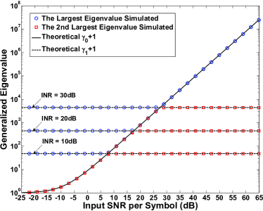
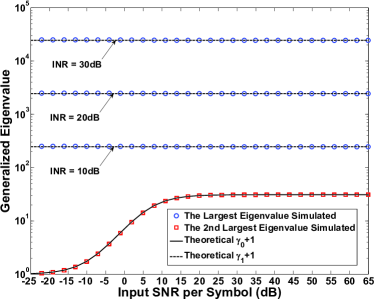
Refer to caption
(a) Maximin scheme
Refer to caption
(b) PAPC scheme
Figure 6: The largest and second largest generalized eigenvalues of the Maximin scheme vs SNR under two periodical noises.
Refer to caption
(a) Case I: below threshold (SNR=10.1SNR10.1\textsf{SNR}\!\!=\!\!-10.1dB, INR=30INR30\textrm{INR}\!\!=\!\!30dB)
Refer to caption
(b) Case II: above threshold (SNR=40.9SNR40.9\textsf{SNR}\!\!=\!\!40.9dB, INR=30INR30\textrm{INR}\!\!=\!\!30dB)
Figure 7: The array patterns corresponding to the Maximin and PAPC under two periodical noises.

In summary, the conventional MPB like Maximin and PAPC work well in the presence of directional white noise, even when the INR is large. However, they are very vulnerable to multiple directional periodical interferers with repeating structures in the time domain and arrive from different directions.

VI Conclusions

Matrix pair beamformer (MPB) is a general framework we proposed to model a class of blind beamformers that exploit the temporal signature of the signal of interest (SOI). It has the advantages only relying on the second order statistics to achieve blind processing. In this paper, we have analyzed the mechanism of MPB with matrix mismatch, and showed how it worked “blindly”. We have discovered that there is a threshold effect in MPB, i.e. the beamformer would fail completely if the SOI’s input SNR is below that threshold. Meanwhile, its normalized output SINR has been derived as the performance measure, and the threshold SNR has also been predicted. We have also observed that the existence of infinite generalized eigenvalue in what is called noise free pair makes the threshold increase unboundedly with the interference power. This is highly probable when there are multiple periodical interferers. All our theoretical analysis matches with the simulation results very well.

Our analysis indicates that the conventional MPB is very vulnerable to multiple periodical interferers. Moreover, it also implies the importance of choosing the appropriate projection space for the interference channel. And we will address this issue in another paper[36].

Appendix A Approximation of λmaxsubscript𝜆max\lambda_{\mathrm{max}} and γisubscript𝛾𝑖\gamma_{i}

A-A Approximation of λmaxsubscript𝜆max\lambda_{\mathrm{max}}

Since similarity transform does not change the eigenvalues, we can apply it to 𝐌𝐌\mathbf{M} before using Lemma 2. As we will see later, the bounds derived in this way can be surprisingly tight. Though any transform matrix can be used, we prefer the following diagonal matrix that can preserve the diagonal terms of 𝐌𝐌\mathbf{M}

𝐅=diag{1,f1,f2,,fD},(fi>0,i=1,2,,D)𝐅diag1subscript𝑓1subscript𝑓2subscript𝑓𝐷formulae-sequencesubscript𝑓𝑖0𝑖12𝐷\displaystyle\mathbf{F}=\mathrm{diag}\{1,f_{1},f_{2},\ldots,f_{D}\},\quad(f_{i}>0,\;i=1,2,\ldots,D)

Applying it to 𝐌𝐌\mathbf{M} in (33) and using Lemma 2, we can have the following Gerschgorin disks for 𝐅𝐌𝐅1superscript𝐅𝐌𝐅1\mathbf{F}\mathbf{M}\mathbf{F}^{-1}:

Gisubscript𝐺𝑖\displaystyle G_{i} ={λ:|λ(γi+1)|<Ri(𝐅)},i=0,1,2,,D,formulae-sequenceabsentconditional-set𝜆𝜆subscript𝛾𝑖1subscript𝑅𝑖𝐅𝑖012𝐷\displaystyle=\{\lambda:\;|\lambda-(\gamma_{i}+1)|<R_{i}(\mathbf{F})\},\qquad i=0,1,2,\ldots,D,

where the radii of the disks are

R0(𝐅)subscript𝑅0𝐅\displaystyle R_{0}(\mathbf{F}) =γ0σ2Li=1D|ψTi|1fiabsentsubscript𝛾0superscript𝜎2𝐿superscriptsubscript𝑖1𝐷subscript𝜓subscript𝑇𝑖1subscript𝑓𝑖\displaystyle=\gamma_{0}\sqrt{\frac{\sigma^{2}}{L}}\sum_{i=1}^{D}|\psi_{T_{i}}|\frac{1}{f_{i}} (51)
Ri(𝐅)subscript𝑅𝑖𝐅\displaystyle R_{i}(\mathbf{F}) =γiσ2L|ψTi|sgn(γi)LβNSNR+1fi,1iD,formulae-sequenceabsentsubscript𝛾𝑖superscript𝜎2𝐿subscript𝜓subscript𝑇𝑖sgnsubscript𝛾𝑖𝐿𝛽𝑁SNR1subscript𝑓𝑖1𝑖𝐷\displaystyle=\gamma_{i}\frac{\sqrt{\frac{\sigma^{2}}{L}}|\psi_{T_{i}}|\cdot\mathrm{sgn}(\gamma_{i})}{\frac{L\beta}{N}\textsf{SNR}+1}f_{i},\quad 1\leq i\leq D, (52)

with ψTisubscript𝜓subscript𝑇𝑖\psi_{T_{i}} being the i𝑖ith component of 𝝍Tsubscript𝝍𝑇\bm{\psi}_{T}. Now, we are going to optimize f1,,fDsubscript𝑓1subscript𝑓𝐷f_{1},\ldots,f_{D}. To derive an effective bound for λmaxsubscript𝜆max\lambda_{\mathrm{max}}, we should ensure the rightmost disk is separated from the others (c.f. Lemma 2). Therefore, our criterion for finding the optimal 𝐅𝐅\mathbf{F} is minimizing the radius of the rightmost Gerschgorin disk subject to the constraint that it is separated from all the remaining ones. Depending on γ0+1>γ1+1subscript𝛾01subscript𝛾11\gamma_{0}+1>\gamma_{1}+1 or γ0+1<γ1+1subscript𝛾01subscript𝛾11\gamma_{0}+1<\gamma_{1}+1, the rightmost disk might be G0subscript𝐺0G_{0} or G1subscript𝐺1G_{1}, and we now discuss them separately.

If γ0+1>γ1+1subscript𝛾01subscript𝛾11\gamma_{0}+1>\gamma_{1}+1, then G0subscript𝐺0G_{0} is the rightmost disk, and we can formulate the optimization of 𝐅𝐅\mathbf{F} as

min\displaystyle\min~{} R0(𝐅)=γ0σ2Li=1D|ψTi|1fisubscript𝑅0𝐅subscript𝛾0superscript𝜎2𝐿superscriptsubscript𝑖1𝐷subscript𝜓subscript𝑇𝑖1subscript𝑓𝑖\displaystyle~{}R_{0}(\mathbf{F})=\gamma_{0}\sqrt{\frac{\sigma^{2}}{L}}\sum_{i=1}^{D}|\psi_{T_{i}}|\frac{1}{f_{i}} (53)
s.t.formulae-sequencest\displaystyle\mathrm{s.t.}~{} γi+1+Ri(F)γ0+1R0(𝐅),1iD.formulae-sequencesubscript𝛾𝑖1subscript𝑅𝑖𝐹subscript𝛾01subscript𝑅0𝐅1𝑖𝐷\displaystyle~{}\gamma_{i}+1+R_{i}(F)\leq\gamma_{0}+1-R_{0}(\mathbf{F}),\quad 1\leq i\leq D. (54)

To minimize R0(𝐅)subscript𝑅0𝐅R_{0}(\mathbf{F}), we want f1,,fDsubscript𝑓1subscript𝑓𝐷f_{1},\ldots,f_{D} to be as large as possible. But this will increase the radius of G1,,GDsubscript𝐺1subscript𝐺𝐷G_{1},\ldots,G_{D}, and to avoid connecting G0subscript𝐺0G_{0}, they cannot be too large. In fact, f1,,fDsubscript𝑓1subscript𝑓𝐷f_{1},\ldots,f_{D} have different importance in this tradeoff. Since γ0>>γDsubscript𝛾0subscript𝛾𝐷\gamma_{0}>\ldots>\gamma_{D}, G2,,GDsubscript𝐺2subscript𝐺𝐷G_{2},\ldots,G_{D} are farther away from G0subscript𝐺0G_{0} than G1subscript𝐺1G_{1}. Therefore, f2,,fDsubscript𝑓2subscript𝑓𝐷f_{2},\ldots,f_{D} can be reasonably larger than f1subscript𝑓1f_{1} when keeping separate from G0subscript𝐺0G_{0}. Thus, to simplify analysis, we can ignore all the terms except |ψT1|/f1subscript𝜓subscript𝑇1subscript𝑓1|\psi_{T_{1}}|/f_{1} in R0(𝐅)subscript𝑅0𝐅R_{0}(\mathbf{F}), i.e. R0(𝐅)γ0σ2L|ψT1|f1subscript𝑅0𝐅subscript𝛾0superscript𝜎2𝐿subscript𝜓subscript𝑇1subscript𝑓1R_{0}(\mathbf{F})\approx\gamma_{0}\sqrt{\frac{\sigma^{2}}{L}}\frac{|\psi_{T_{1}}|}{f_{1}} in (53) and (54), and only the constraint for i=1𝑖1i=1 is effective in (54). Then, the problem can be reduced to

min\displaystyle\min~{} R0(𝐅)γ0σ2L|ψT1|1f1subscript𝑅0𝐅subscript𝛾0superscript𝜎2𝐿subscript𝜓subscript𝑇11subscript𝑓1\displaystyle~{}R_{0}(\mathbf{F})\approx\gamma_{0}\sqrt{\frac{\sigma^{2}}{L}}|\psi_{T_{1}}|\frac{1}{f_{1}}
s.t.formulae-sequencest\displaystyle\mathrm{s.t.}~{} γ1σ2L|ψT1|sgn(γ1)LβNSNR+1f12(γ0γ1)f1+γ0σ2L|ψT1|0.subscript𝛾1superscript𝜎2𝐿subscript𝜓subscript𝑇1sgnsubscript𝛾1𝐿𝛽𝑁SNR1superscriptsubscript𝑓12subscript𝛾0subscript𝛾1subscript𝑓1subscript𝛾0superscript𝜎2𝐿subscript𝜓subscript𝑇10\displaystyle~{}\gamma_{1}\frac{\sqrt{\frac{\sigma^{2}}{L}}|\psi_{T_{1}}|\cdot\mathrm{sgn}(\gamma_{1})}{\frac{L\beta}{N}\textsf{SNR}+1}f_{1}^{2}-(\gamma_{0}-\gamma_{1})f_{1}+\gamma_{0}\sqrt{\frac{\sigma^{2}}{L}}|\psi_{T_{1}}|\leq 0.

This is a simple convex optimization problem, feasible when γ1γ0(,1+2δ(1+2δ)21]subscript𝛾1subscript𝛾012𝛿superscript12𝛿21\frac{\gamma_{1}}{\gamma_{0}}\in(-\infty,1+2\delta-\sqrt{(1+2\delta)^{2}-1}], where δσ2L|ψT1|2/(LβNSNR+1)1𝛿superscript𝜎2𝐿superscriptsubscript𝜓subscript𝑇12𝐿𝛽𝑁SNR1much-less-than1\delta\triangleq\frac{\sigma^{2}}{L}|\psi_{T_{1}}|^{2}/(\frac{L\beta}{N}\textsf{SNR}+1)\ll 1. Thus, we can easily solve the above optimization and get

|λmax(γ0+1)|<γ0f(γ1γ0)subscript𝜆maxsubscript𝛾01subscript𝛾0𝑓subscript𝛾1subscript𝛾0\displaystyle|\lambda_{\mathrm{max}}-(\gamma_{0}+1)|<\gamma_{0}\cdot f\left(\frac{\gamma_{1}}{\gamma_{0}}\right)

where f(x)12[1x(1x)24δ|x|]𝑓𝑥12delimited-[]1𝑥superscript1𝑥24𝛿𝑥f(x)\triangleq\frac{1}{2}[1\!-\!x\!-\!\sqrt{(1\!-\!x)^{2}\!-\!4\delta|x|}] with x(,12δ+δ2+2δ][1+2δ+δ2+2δ,+)𝑥12𝛿superscript𝛿22𝛿12𝛿superscript𝛿22𝛿x\in(-\infty,1\!-\!2\sqrt{\delta\!+\!\delta^{2}}\!+\!2\delta]\!\cup\![1\!+\!2\sqrt{\delta\!+\!\delta^{2}}\!+\!2\delta,+\infty). Furthermore, by taking the derivative of f(x)𝑓𝑥f(x), we can easily get 0f(x)max{δ,δ2+δδ}10𝑓𝑥𝛿superscript𝛿2𝛿𝛿much-less-than10\!\!\leq\!\!f(x)\!\!\leq\!\!\max\{\delta,\sqrt{\delta^{2}\!\!+\!\!\delta}\!\!-\!\!\delta\}\!\!\ll\!\!1 when x(,12δ+δ2+2δ]𝑥12𝛿superscript𝛿22𝛿x\in(-\infty,1\!-\!2\sqrt{\delta\!+\!\delta^{2}}\!+\!2\delta].

If γ0+1<γ1+1subscript𝛾01subscript𝛾11\gamma_{0}+1<\gamma_{1}+1, then G1subscript𝐺1G_{1} is the rightmost disk and γ1>0subscript𝛾10\gamma_{1}>0. The optimization problem is

min\displaystyle\min~{} R1(𝐅)=γ1σ2L|ψT1|LβNSNR+1f1subscript𝑅1𝐅subscript𝛾1superscript𝜎2𝐿subscript𝜓subscript𝑇1𝐿𝛽𝑁SNR1subscript𝑓1\displaystyle~{}R_{1}(\mathbf{F})=\gamma_{1}\frac{\sqrt{\frac{\sigma^{2}}{L}}|\psi_{T_{1}}|}{\frac{L\beta}{N}\textsf{SNR}+1}f_{1} (55)
s.t.formulae-sequencest\displaystyle\mathrm{s.t.}~{} γ0+1+R0(F)γ1+1R1(𝐅),subscript𝛾01subscript𝑅0𝐹subscript𝛾11subscript𝑅1𝐅\displaystyle~{}\gamma_{0}+1+R_{0}(F)\leq\gamma_{1}+1-R_{1}(\mathbf{F}), (56)
γi+1+Ri(F)γ1+1R1(𝐅),2iD.formulae-sequencesubscript𝛾𝑖1subscript𝑅𝑖𝐹subscript𝛾11subscript𝑅1𝐅2𝑖𝐷\displaystyle~{}\gamma_{i}+1+R_{i}(F)\leq\gamma_{1}+1-R_{1}(\mathbf{F}),\quad 2\leq i\leq D. (57)

According to (51) and (52), f1subscript𝑓1f_{1} should be as small as possible to minimize R1(𝐅)subscript𝑅1𝐅R_{1}(\mathbf{F}) in (55), (56) and (57). However, this will increase R0(𝐅)subscript𝑅0𝐅R_{0}(\mathbf{F}) in (56), making G0subscript𝐺0G_{0} connect with G1subscript𝐺1G_{1}. Therefore, f1subscript𝑓1f_{1} cannot be arbitrarily small. On the other hand, f2,,fDsubscript𝑓2subscript𝑓𝐷f_{2},\ldots,f_{D} should be as large as possible to reduce R0(𝐅)subscript𝑅0𝐅R_{0}(\mathbf{F}) in (56) while keeping (57) valid. As a result, |ψT1|/f1subscript𝜓subscript𝑇1subscript𝑓1|\psi_{T_{1}}|/f_{1} is still the dominant term in R0(𝐅)subscript𝑅0𝐅R_{0}(\mathbf{F}) (c.f. (51)) and the key point here remains the tradeoff between R1(𝐅)subscript𝑅1𝐅R_{1}(\mathbf{F}) and R0(𝐅)subscript𝑅0𝐅R_{0}(\mathbf{F}). In other words, the optimization becomes

min\displaystyle\min~{} R1(𝐅)=γ1σ2L|ψT1|LβNSNR+1f1subscript𝑅1𝐅subscript𝛾1superscript𝜎2𝐿subscript𝜓subscript𝑇1𝐿𝛽𝑁SNR1subscript𝑓1\displaystyle~{}R_{1}(\mathbf{F})=\gamma_{1}\frac{\sqrt{\frac{\sigma^{2}}{L}}|\psi_{T_{1}}|}{\frac{L\beta}{N}\textsf{SNR}+1}f_{1}
s.t.formulae-sequencest\displaystyle\mathrm{s.t.}~{} γ1σ2L|ψT1|LβNSNR+1f12(γ1γ0)f1+γ0σ2L|ψT1|0.subscript𝛾1superscript𝜎2𝐿subscript𝜓subscript𝑇1𝐿𝛽𝑁SNR1superscriptsubscript𝑓12subscript𝛾1subscript𝛾0subscript𝑓1subscript𝛾0superscript𝜎2𝐿subscript𝜓subscript𝑇10\displaystyle~{}\gamma_{1}\frac{\sqrt{\frac{\sigma^{2}}{L}}|\psi_{T_{1}}|}{\frac{L\beta}{N}\textsf{SNR}+1}f_{1}^{2}-(\gamma_{1}-\gamma_{0})f_{1}+\gamma_{0}\sqrt{\frac{\sigma^{2}}{L}}|\psi_{T_{1}}|\leq 0.

The feasible region for this convex optimization is γ1γ0[1+2δ+(1+2δ)21,+)subscript𝛾1subscript𝛾012𝛿superscript12𝛿21\frac{\gamma_{1}}{\gamma_{0}}\in[1+2\delta+\sqrt{(1+2\delta)^{2}-1},+\infty), with δ𝛿\delta defined in the previous case. By solving it, we can finally get the bound for λmaxsubscript𝜆max\lambda_{\mathrm{max}} as

|λmax(γ1+1)|γ1f(γ0γ1)subscript𝜆maxsubscript𝛾11subscript𝛾1𝑓subscript𝛾0subscript𝛾1\displaystyle|\lambda_{\mathrm{max}}-(\gamma_{1}+1)|\leq\gamma_{1}\cdot f\left(\frac{\gamma_{0}}{\gamma_{1}}\right)

where f(x)𝑓𝑥f(x) is the same as in the previous case.

A-B Approximation of γisubscript𝛾𝑖\gamma_{i}

Then, we discuss the approximation of γisubscript𝛾𝑖\gamma_{i}. By substituting (5) into (30) and using matrix inversion lemma, we can have the equivalent equation of (30) as

det(𝐀IH𝐑1𝐀I)1det{λ𝐈[𝐀IH𝐐1𝐀Iσ2𝐀IH𝐐1𝐚0𝐚0H𝐐1𝐀I1+σ2𝐚0H𝐐1𝐚0]𝚽Δ}=0superscriptsuperscriptsubscript𝐀𝐼𝐻superscriptsubscript𝐑1subscript𝐀𝐼1𝜆𝐈delimited-[]superscriptsubscript𝐀𝐼𝐻superscriptsubscript𝐐1subscript𝐀𝐼superscriptsubscript𝜎2superscriptsubscript𝐀𝐼𝐻superscriptsubscript𝐐1subscript𝐚0superscriptsubscript𝐚0𝐻superscriptsubscript𝐐1subscript𝐀𝐼1superscriptsubscript𝜎2superscriptsubscript𝐚0𝐻superscriptsubscript𝐐1subscript𝐚0subscript𝚽Δ0\displaystyle\det(\mathbf{A}_{I}^{H}\mathbf{R}_{\mathcal{I}}^{-1}\mathbf{A}_{I})^{-1}\cdot\det\left\{\lambda\mathbf{I}-\left[\mathbf{A}_{I}^{H}\mathbf{Q}_{\mathcal{I}}^{-1}\mathbf{A}_{I}-\frac{\sigma_{\mathcal{I}}^{2}\mathbf{A}_{I}^{H}\mathbf{Q}_{\mathcal{I}}^{-1}\mathbf{a}_{0}\cdot\mathbf{a}_{0}^{H}\mathbf{Q}_{\mathcal{I}}^{-1}\mathbf{A}_{I}}{1+\sigma_{\mathcal{I}}^{2}\mathbf{a}_{0}^{H}\mathbf{Q}_{\mathcal{I}}^{-1}\mathbf{a}_{0}}\right]\bm{\Phi}_{\Delta}\right\}=0 (58)

To further reduce the above expression, we need factorizations of 𝐀IH𝐐1𝐀Isuperscriptsubscript𝐀𝐼𝐻superscriptsubscript𝐐1subscript𝐀𝐼\mathbf{A}_{I}^{H}\mathbf{Q}_{\mathcal{I}}^{-1}\mathbf{A}_{I} and 𝚽Δsubscript𝚽Δ\bm{\Phi}_{\Delta} like (28). Let σ02=0superscriptsubscript𝜎subscript020\sigma_{\mathcal{I}_{0}}^{2}=0 in (28). Then, 𝐑=𝐐subscript𝐑subscript𝐐\mathbf{R}_{\mathcal{I}}=\mathbf{Q}_{\mathcal{I}}, and (28) become

𝐓0H𝚽Δ𝐓0=𝚪0,𝐓0H(𝐀IH𝐐1𝐀I)1𝐓0=𝐈.formulae-sequencesubscriptsuperscript𝐓𝐻0subscript𝚽Δsubscript𝐓0subscript𝚪0subscriptsuperscript𝐓𝐻0superscriptsuperscriptsubscript𝐀𝐼𝐻superscriptsubscript𝐐1subscript𝐀𝐼1subscript𝐓0𝐈\displaystyle\mathbf{T}^{H}_{0}\bm{\Phi}_{\Delta}\mathbf{T}_{0}=\bm{\Gamma}_{0},\qquad\mathbf{T}^{H}_{0}(\mathbf{A}_{I}^{H}\mathbf{Q}_{\mathcal{I}}^{-1}\mathbf{A}_{I})^{-1}\mathbf{T}_{0}=\mathbf{I}.

where 𝐓0subscript𝐓0\mathbf{T}_{0} and 𝚪0subscript𝚪0\bm{\Gamma}_{0} are the counterparts of 𝐓𝐓\mathbf{T} and 𝚪𝚪\bm{\Gamma}, respectively. Substituting them into (58), we have

det(𝐀IH𝐑1𝐀I)1det{λ𝐈[𝐈σ2𝝍~T0𝝍~T0H1+σ2𝐚0H𝐐1𝐚0]𝚪0}=0superscriptsuperscriptsubscript𝐀𝐼𝐻superscriptsubscript𝐑1subscript𝐀𝐼1𝜆𝐈delimited-[]𝐈superscriptsubscript𝜎2subscript~𝝍subscript𝑇0superscriptsubscript~𝝍subscript𝑇0𝐻1superscriptsubscript𝜎2superscriptsubscript𝐚0𝐻superscriptsubscript𝐐1subscript𝐚0subscript𝚪00\displaystyle\det(\mathbf{A}_{I}^{H}\mathbf{R}_{\mathcal{I}}^{-1}\mathbf{A}_{I})^{-1}\cdot\det\left\{\lambda\mathbf{I}-\left[\mathbf{I}-\frac{\sigma_{\mathcal{I}}^{2}\tilde{\bm{\psi}}_{T_{0}}\tilde{\bm{\psi}}_{T_{0}}^{H}}{1+\sigma_{\mathcal{I}}^{2}\mathbf{a}_{0}^{H}\mathbf{Q}_{\mathcal{I}}^{-1}\mathbf{a}_{0}}\right]\bm{\Gamma}_{0}\right\}=0

where 𝝍~T0=𝐓01𝐀IH𝐐1𝐚0subscript~𝝍subscript𝑇0superscriptsubscript𝐓01superscriptsubscript𝐀𝐼𝐻superscriptsubscript𝐐1subscript𝐚0\tilde{\bm{\psi}}_{T_{0}}=\mathbf{T}_{0}^{-1}\mathbf{A}_{I}^{H}\mathbf{Q}_{\mathcal{I}}^{-1}\mathbf{a}_{0} is the counterpart of 𝝍~Tsubscript~𝝍𝑇\tilde{\bm{\psi}}_{T} when σ02=0superscriptsubscript𝜎subscript020\sigma_{\mathcal{I}_{0}}^{2}=0. By letting SNR=0SNR0\textsf{SNR}=0 in Lemma 1, 𝐑subscript𝐑\mathbf{R}_{\mathcal{I}} becomes 𝐐subscript𝐐\mathbf{Q}_{\mathcal{I}} and we can have 𝐚0H𝐐1𝐚0L/σ2superscriptsubscript𝐚0𝐻superscriptsubscript𝐐1subscript𝐚0𝐿superscript𝜎2\mathbf{a}_{0}^{H}\mathbf{Q}_{\mathcal{I}}^{-1}\mathbf{a}_{0}\approx L/\sigma^{2} and 𝝍T02=Lκ0/σ2L/σ2superscriptnormsubscript𝝍subscript𝑇02𝐿subscript𝜅0superscript𝜎2much-less-than𝐿superscript𝜎2\|\bm{\psi}_{T_{0}}\|^{2}=L\kappa_{0}/\sigma^{2}\ll L/\sigma^{2}. Therefore, by the similar argument of λmaxsubscript𝜆max\lambda_{\mathrm{max}} using Gerschgorin theorem, we can have γiλi,0subscript𝛾𝑖subscript𝜆𝑖0\gamma_{i}\approx\lambda_{i,0}, where λi,0subscript𝜆𝑖0\lambda_{i,0} is the i𝑖ith diagonal term of 𝚪0subscript𝚪0\bm{\Gamma}_{0}, namely, the i𝑖ith eigenvalue of (𝚽Δ,(𝐀IH𝐐1𝐀I)1)subscript𝚽Δsuperscriptsuperscriptsubscript𝐀𝐼𝐻superscriptsubscript𝐐1subscript𝐀𝐼1(\bm{\Phi}_{\Delta},(\mathbf{A}_{I}^{H}\mathbf{Q}_{\mathcal{I}}^{-1}\mathbf{A}_{I})^{-1}). In fact, there is a correspondence between λi,0subscript𝜆𝑖0\lambda_{i,0} and the generalized eigenvalue of (𝐐𝒮𝐐,𝐐)subscript𝐐𝒮subscript𝐐subscript𝐐(\mathbf{Q}_{\mathcal{S}}-\mathbf{Q}_{\mathcal{I}},\mathbf{Q}_{\mathcal{I}}). By (31),

det{λ(𝐀IH𝐐1𝐀I)1𝚽Δ}𝜆superscriptsuperscriptsubscript𝐀𝐼𝐻superscriptsubscript𝐐1subscript𝐀𝐼1subscript𝚽Δ\displaystyle\det\left\{\lambda(\mathbf{A}_{I}^{H}\mathbf{Q}_{\mathcal{I}}^{-1}\mathbf{A}_{I})^{-1}-\bm{\Phi}_{\Delta}\right\} =λDLdet(𝐀IH𝐐1𝐀I)1det𝐐1det{λ𝐐𝐀I𝚽Δ𝐀IH}.absentsuperscript𝜆𝐷𝐿superscriptsuperscriptsubscript𝐀𝐼𝐻superscriptsubscript𝐐1subscript𝐀𝐼1superscriptsubscript𝐐1𝜆subscript𝐐subscript𝐀𝐼subscript𝚽Δsuperscriptsubscript𝐀𝐼𝐻\displaystyle=\lambda^{D-L}\cdot\det(\mathbf{A}_{I}^{H}\mathbf{Q}_{\mathcal{I}}^{-1}\mathbf{A}_{I})^{-1}\det\mathbf{Q}_{\mathcal{I}}^{-1}\cdot\det\{\lambda\mathbf{Q}_{\mathcal{I}}-\mathbf{A}_{I}\bm{\Phi}_{\Delta}\mathbf{A}_{I}^{H}\}.

Since 𝐐𝒮𝐐=𝐀I𝚽Δ𝐀IHsubscript𝐐𝒮subscript𝐐subscript𝐀𝐼subscript𝚽Δsuperscriptsubscript𝐀𝐼𝐻\mathbf{Q}_{\mathcal{S}}-\mathbf{Q}_{\mathcal{I}}=\mathbf{A}_{I}\bm{\Phi}_{\Delta}\mathbf{A}_{I}^{H}, the above expression implies that (𝚽Δ,(𝐀IH𝐐1𝐀I)1)subscript𝚽Δsuperscriptsuperscriptsubscript𝐀𝐼𝐻superscriptsubscript𝐐1subscript𝐀𝐼1(\bm{\Phi}_{\Delta},(\mathbf{A}_{I}^{H}\mathbf{Q}_{\mathcal{I}}^{-1}\mathbf{A}_{I})^{-1}) has the same eigenvalues as (𝐐𝒮𝐐,𝐐)subscript𝐐𝒮subscript𝐐subscript𝐐(\mathbf{Q}_{\mathcal{S}}-\mathbf{Q}_{\mathcal{I}},\mathbf{Q}_{\mathcal{I}}) except for multiplicity of zeros. Thus, we can estimate γisubscript𝛾𝑖\gamma_{i} like this: 1) take out all nonzero eigenvalues of (𝐐𝒮𝐐,𝐐)subscript𝐐𝒮subscript𝐐subscript𝐐(\mathbf{Q}_{\mathcal{S}}-\mathbf{Q}_{\mathcal{I}},\mathbf{Q}_{\mathcal{I}}), 2) pad them up to D𝐷D eigenvalues with zeros, 3) order them decreasingly to get λ1,0,,λD,0subscript𝜆10subscript𝜆𝐷0\lambda_{1,0},\ldots,\lambda_{D,0}, and 4) let γiλi,0subscript𝛾𝑖subscript𝜆𝑖0\gamma_{i}\approx\lambda_{i,0}.

Appendix B Proof of Lemma 3

Substituting the definitions of yS(k)subscript𝑦𝑆𝑘y_{S}(k) and yI(k)subscript𝑦𝐼𝑘y_{I}(k) (c.f. (10)), (6) and (14) into (17) , we can have

G(SNR)GSNR\displaystyle\textsf{G}(\textsf{SNR}) =|𝐰H𝐚0|2𝐰H𝐀I𝚽𝒮𝐀IH𝐰+σ2𝐰21𝐚0H𝐐𝒮1𝐚0|𝐰H𝐚0|2𝐰H𝐀I𝚽𝒮𝐀IH𝐰+σ2𝐰2/Lσ2,absentsuperscriptsuperscript𝐰𝐻subscript𝐚02superscript𝐰𝐻subscript𝐀𝐼subscript𝚽𝒮superscriptsubscript𝐀𝐼𝐻𝐰superscript𝜎2superscriptnorm𝐰21superscriptsubscript𝐚0𝐻superscriptsubscript𝐐𝒮1subscript𝐚0superscriptsuperscript𝐰𝐻subscript𝐚02superscript𝐰𝐻subscript𝐀𝐼subscript𝚽𝒮superscriptsubscript𝐀𝐼𝐻𝐰superscript𝜎2superscriptnorm𝐰2𝐿superscript𝜎2\displaystyle=\frac{|\mathbf{w}^{H}\mathbf{a}_{0}|^{2}}{\mathbf{w}^{H}\mathbf{A}_{I}\bm{\Phi}_{\mathcal{S}}\mathbf{A}_{I}^{H}\mathbf{w}+\sigma^{2}\|\mathbf{w}\|^{2}}\frac{1}{\mathbf{a}_{0}^{H}\mathbf{Q}_{\mathcal{S}}^{-1}\mathbf{a}_{0}}\approx\frac{|\mathbf{w}^{H}\mathbf{a}_{0}|^{2}}{\mathbf{w}^{H}\mathbf{A}_{I}\bm{\Phi}_{\mathcal{S}}\mathbf{A}_{I}^{H}\mathbf{w}+\sigma^{2}\|\mathbf{w}\|^{2}}\big{/}\frac{L}{\sigma^{2}}, (59)

where we used 𝐚0H𝐐𝒮1𝐚0L/σ2superscriptsubscript𝐚0𝐻superscriptsubscript𝐐𝒮1subscript𝐚0𝐿superscript𝜎2\mathbf{a}_{0}^{H}\mathbf{Q}_{\mathcal{S}}^{-1}\mathbf{a}_{0}\!\!\approx\!\!{L}/{\sigma^{2}}, derived by replacing 𝐑subscript𝐑\mathbf{R}_{\mathcal{I}} with 𝐑𝒮subscript𝐑𝒮\mathbf{R}_{\mathcal{S}} and letting σ𝒮02=0superscriptsubscript𝜎subscript𝒮020\sigma_{\mathcal{S}_{0}}^{2}\!\!=\!\!0 in Lemma 1.

To further derive G, we first need the expression for 𝐰2superscriptnorm𝐰2\|\mathbf{w}\|^{2}. The key trick is to recognize that 𝐰(𝐀)𝐰𝐀\mathbf{w}\in\mathcal{R}(\mathbf{A}) so that its projection onto (𝐀)𝐀\mathcal{R}(\mathbf{A}) equals itself, where ()\mathcal{R}(\cdot) is the range space of a matrix and 𝐀[𝐚0𝐀I]𝐀delimited-[]subscript𝐚0subscript𝐀𝐼\mathbf{A}\triangleq[\mathbf{a}_{0}\;\mathbf{A}_{I}]. This can be proved by substituting (7) into (5), applying matrix inversion lemma and pluging it into (27). Furthermore, (𝐀I)subscript𝐀𝐼\mathcal{R}(\mathbf{A}_{I}) is a subspace of (𝐀)𝐀\mathcal{R}(\mathbf{A}) with the dimension lower by one. Thus, (𝐀)=(𝐀)(𝐛^0)𝐀direct-sum𝐀subscript^𝐛0\mathcal{R}(\mathbf{A})\!\!=\!\!\mathcal{R}(\mathbf{A})\!\oplus\!\mathcal{R}(\hat{\mathbf{b}}_{0}), where direct-sum\oplus denotes the direct sum and 𝐛^0subscript^𝐛0\hat{\mathbf{b}}_{0} is the unit vector in (𝐀)𝐀\mathcal{R}(\mathbf{A}) that is orthogonal to (𝐀I)subscript𝐀𝐼\mathcal{R}(\mathbf{A}_{I}). Then, the projection matrix of (𝐀)𝐀\mathcal{R}(\mathbf{A}) can be written as

𝐏A=𝐀I(𝐀IH𝐀I)1𝐀IH+𝐛^0𝐛^0H.subscript𝐏𝐴subscript𝐀𝐼superscriptsuperscriptsubscript𝐀𝐼𝐻subscript𝐀𝐼1superscriptsubscript𝐀𝐼𝐻subscript^𝐛0superscriptsubscript^𝐛0𝐻\displaystyle\mathbf{P}_{A}=\mathbf{A}_{I}(\mathbf{A}_{I}^{H}\mathbf{A}_{I})^{-1}\mathbf{A}_{I}^{H}+\mathbf{\hat{b}}_{0}\mathbf{\hat{b}}_{0}^{H}.

This together with 𝐏A𝐰=𝐰subscript𝐏𝐴𝐰𝐰\mathbf{P}_{A}\mathbf{w}=\mathbf{w} and 𝐏A2=𝐏Asuperscriptsubscript𝐏𝐴2subscript𝐏𝐴\mathbf{P}_{A}^{2}=\mathbf{P}_{A} yields

𝐰2=𝐰H𝐏A𝐰=𝐰H𝐀I(𝐀IH𝐀I)1𝐀IH𝐰+|𝐰H𝐛^0|2superscriptnorm𝐰2superscript𝐰𝐻subscript𝐏𝐴𝐰superscript𝐰𝐻subscript𝐀𝐼superscriptsuperscriptsubscript𝐀𝐼𝐻subscript𝐀𝐼1superscriptsubscript𝐀𝐼𝐻𝐰superscriptsuperscript𝐰𝐻subscript^𝐛02\displaystyle\|\mathbf{w}\|^{2}=\mathbf{w}^{H}\mathbf{P}_{A}\mathbf{w}=\mathbf{w}^{H}\mathbf{A}_{I}(\mathbf{A}_{I}^{H}\mathbf{A}_{I})^{-1}\mathbf{A}_{I}^{H}\mathbf{w}+|\mathbf{w}^{H}\mathbf{\hat{b}}_{0}|^{2} (60)

Assumption 1 in Sec. III-A implies that 𝐚0subscript𝐚0\mathbf{a}_{0} is almost orthogonal to (𝐀I)subscript𝐀𝐼\mathcal{R}(\mathbf{A}_{I}). Thus, it is nearly aligned with 𝐛^0subscript^𝐛0\hat{\mathbf{b}}_{0}, and intuitively, |𝐰H𝐛^0||𝐰H𝐚^0|superscript𝐰𝐻subscript^𝐛0superscript𝐰𝐻subscript^𝐚0|\mathbf{w}^{H}\hat{\mathbf{b}}_{0}|\!\!\approx\!\!|\mathbf{w}^{H}\hat{\mathbf{a}}_{0}|, where 𝐚^0𝐚0/𝐚0subscript^𝐚0subscript𝐚0normsubscript𝐚0\hat{\mathbf{a}}_{0}\!\!\triangleq\!\!\mathbf{a}_{0}/\|\mathbf{a}_{0}\| is the unit vector of 𝐚0subscript𝐚0\mathbf{a}_{0}. To prove it, let 0span{𝐚^0,𝐛^0}subscript0spansubscript^𝐚0subscript^𝐛0\mathcal{R}_{0}\!\!\triangleq\!\!\mathrm{span}\{\hat{\mathbf{a}}_{0},\hat{\mathbf{b}}_{0}\} and {𝐛^0,𝐛^1}subscript^𝐛0subscript^𝐛1\{\hat{\mathbf{b}}_{0},\hat{\mathbf{b}}_{1}\} be the orthonormal basis of 0subscript0\mathcal{R}_{0}. Its projection matrix becomes 𝐏0=𝐛^0𝐛^0H+𝐛^1𝐛^1Hsubscript𝐏subscript0subscript^𝐛0superscriptsubscript^𝐛0𝐻subscript^𝐛1superscriptsubscript^𝐛1𝐻\mathbf{P}_{\mathcal{R}_{0}}\!\!=\!\!\hat{\mathbf{b}}_{0}\hat{\mathbf{b}}_{0}^{H}\!\!+\!\!\hat{\mathbf{b}}_{1}\hat{\mathbf{b}}_{1}^{H}, which satisfies 𝐏0𝐚^0=𝐚^0subscript𝐏subscript0subscript^𝐚0subscript^𝐚0\mathbf{P}_{\mathcal{R}_{0}}\hat{\mathbf{a}}_{0}\!\!=\!\!\hat{\mathbf{a}}_{0} and 𝐏0𝐛^0=𝐛^0subscript𝐏subscript0subscript^𝐛0subscript^𝐛0\mathbf{P}_{\mathcal{R}_{0}}\hat{\mathbf{b}}_{0}\!\!=\!\!\hat{\mathbf{b}}_{0}. Define 𝐰0=𝐏0𝐰/𝐏0𝐰subscript𝐰0subscript𝐏subscript0𝐰normsubscript𝐏subscript0𝐰\mathbf{w}_{0}\!\!=\!\!\mathbf{P}_{\mathcal{R}_{0}}\mathbf{w}/\|\mathbf{P}_{\mathcal{R}_{0}}\mathbf{w}\|. Then,

|𝐰H𝐛^0|2superscriptsuperscript𝐰𝐻subscript^𝐛02\displaystyle|\mathbf{w}^{H}\mathbf{\hat{b}}_{0}|^{2} =|𝐰H𝐚^0|2+[|𝐰H𝐛^0|2|𝐰H𝐚^0|2]=|𝐰H𝐚^0|2+[|𝐰H𝐏0𝐛^0|2|𝐰H𝐏0𝐏0𝐚^0|2]absentsuperscriptsuperscript𝐰𝐻subscript^𝐚02delimited-[]superscriptsuperscript𝐰𝐻subscript^𝐛02superscriptsuperscript𝐰𝐻subscript^𝐚02superscriptsuperscript𝐰𝐻subscript^𝐚02delimited-[]superscriptsuperscript𝐰𝐻subscript𝐏subscript0subscript^𝐛02superscriptsuperscript𝐰𝐻subscript𝐏subscript0subscript𝐏subscript0subscript^𝐚02\displaystyle=|\mathbf{w}^{H}\mathbf{\hat{a}}_{0}|^{2}\!\!+\!\!\left[|\mathbf{w}^{H}\mathbf{\hat{b}}_{0}|^{2}\!\!-\!\!|\mathbf{w}^{H}\mathbf{\hat{a}}_{0}|^{2}\right]=|\mathbf{w}^{H}\mathbf{\hat{a}}_{0}|^{2}\!\!+\!\!\left[|\mathbf{w}^{H}\mathbf{P}_{\mathcal{R}_{0}}\mathbf{\hat{b}}_{0}|^{2}\!\!-\!\!|\mathbf{w}^{H}\mathbf{P}_{\mathcal{R}_{0}}\mathbf{P}_{\mathcal{R}_{0}}\mathbf{\hat{a}}_{0}|^{2}\right]
=|𝐰H𝐚^0|2+𝐏0𝐰2[|𝐰0H𝐛^0|2|𝐰0H𝐛^0𝐛^0H𝐚^0+𝐰0H𝐛^1𝐛^1H𝐚^0|2]absentsuperscriptsuperscript𝐰𝐻subscript^𝐚02superscriptnormsubscript𝐏subscript0𝐰2delimited-[]superscriptsuperscriptsubscript𝐰0𝐻subscript^𝐛02superscriptsuperscriptsubscript𝐰0𝐻subscript^𝐛0superscriptsubscript^𝐛0𝐻subscript^𝐚0superscriptsubscript𝐰0𝐻subscript^𝐛1superscriptsubscript^𝐛1𝐻subscript^𝐚02\displaystyle=|\mathbf{w}^{H}\mathbf{\hat{a}}_{0}|^{2}\!\!+\!\!\|\mathbf{P}_{\mathcal{R}_{0}}\mathbf{w}\|^{2}\left[|\mathbf{w}_{0}^{H}\mathbf{\hat{b}}_{0}|^{2}\!\!-\!\!|\mathbf{w}_{0}^{H}\hat{\mathbf{b}}_{0}\cdot\hat{\mathbf{b}}_{0}^{H}\mathbf{\hat{a}}_{0}\!\!+\!\!\mathbf{w}_{0}^{H}\hat{\mathbf{b}}_{1}\cdot\hat{\mathbf{b}}_{1}^{H}\mathbf{\hat{a}}_{0}|^{2}\right]
=|𝐰H𝐚^0|2+𝐏0𝐰2cosϕIcos(ϕ1+2ϕI)absentsuperscriptsuperscript𝐰𝐻subscript^𝐚02superscriptnormsubscript𝐏subscript0𝐰2subscriptitalic-ϕ𝐼subscriptitalic-ϕ12subscriptitalic-ϕ𝐼\displaystyle=|\mathbf{w}^{H}\mathbf{\hat{a}}_{0}|^{2}\!\!+\!\!\|\mathbf{P}_{\mathcal{R}_{0}}\mathbf{w}\|^{2}\cdot\cos\phi_{I}\cdot\cos(\phi_{1}+2\phi_{I}) (61)

where ϕIsubscriptitalic-ϕ𝐼\phi_{I} is the angle between 𝐚^0subscript^𝐚0\hat{\mathbf{a}}_{0} and (𝐀I)subscript𝐀𝐼\mathcal{R}(\mathbf{A}_{I}), and ϕ1subscriptitalic-ϕ1\phi_{1} is the angle between 𝐚^0subscript^𝐚0\hat{\mathbf{a}}_{0} and 𝐛^0subscript^𝐛0\hat{\mathbf{b}}_{0}. And the derivation of the last step in (61) involves some simple trigonometry identities like product-to-sum formula. Let 𝚿I𝐀IH𝐀I/Lsubscript𝚿𝐼superscriptsubscript𝐀𝐼𝐻subscript𝐀𝐼𝐿\boldsymbol{\Psi}_{I}\!\!\triangleq\!\!\mathbf{A}_{I}^{H}\mathbf{A}_{I}/L. Combining (60), (61), 𝐏0𝐰𝐰normsubscript𝐏subscript0𝐰norm𝐰\|\mathbf{P}_{\mathcal{R}_{0}}\mathbf{w}\|\!\!\leq\!\!\|\mathbf{w}\| and |cosϕI|1much-less-thansubscriptitalic-ϕ𝐼1|\cos\phi_{I}|\!\!\ll\!\!1 (c.f. Assumption 1), we can have

𝐰2superscriptnorm𝐰2\displaystyle\|\mathbf{w}\|^{2} =1L[|𝐚0H𝐰|2+𝐰H𝐀I𝚿I1𝐀IH𝐰]1𝐏0𝐰2𝐰2cosϕIcos(ϕ1+2ϕI)1L[|𝐚0H𝐰|2+𝐰H𝐀I𝚿I1𝐀IH𝐰],absent1𝐿delimited-[]superscriptsuperscriptsubscript𝐚0𝐻𝐰2superscript𝐰𝐻subscript𝐀𝐼superscriptsubscript𝚿𝐼1superscriptsubscript𝐀𝐼𝐻𝐰1superscriptnormsubscript𝐏subscript0𝐰2superscriptnorm𝐰2subscriptitalic-ϕ𝐼subscriptitalic-ϕ12subscriptitalic-ϕ𝐼1𝐿delimited-[]superscriptsuperscriptsubscript𝐚0𝐻𝐰2superscript𝐰𝐻subscript𝐀𝐼superscriptsubscript𝚿𝐼1superscriptsubscript𝐀𝐼𝐻𝐰\displaystyle=\frac{\frac{1}{L}\left[|\mathbf{a}_{0}^{H}\mathbf{w}|^{2}+\mathbf{w}^{H}\mathbf{A}_{I}\boldsymbol{\Psi}_{I}^{-1}\mathbf{A}_{I}^{H}\mathbf{w}\right]}{1-\frac{\|\mathbf{P}_{\mathcal{R}_{0}}\mathbf{w}\|^{2}}{\|\mathbf{w}\|^{2}}\cdot\cos\phi_{I}\cdot\cos(\phi_{1}+2\phi_{I})}\approx\frac{1}{L}\left[|\mathbf{a}_{0}^{H}\mathbf{w}|^{2}+\mathbf{w}^{H}\mathbf{A}_{I}\boldsymbol{\Psi}_{I}^{-1}\mathbf{A}_{I}^{H}\mathbf{w}\right],

where we also used 𝐚02=Lsuperscriptnormsubscript𝐚02𝐿\|\mathbf{a}_{0}\|^{2}\!\!=\!\!L in Assumption 2. Substitute the above expression back to (59), and we get

G(SNR)|𝐰H𝐚0|2𝐰H𝐀I[Lσ2𝚽𝒮+𝚿I1]𝐀IH𝐰+|𝐰H𝐚0|2.\displaystyle\textsf{G}(\textsf{SNR})\approx\ \frac{|\mathbf{w}^{H}\mathbf{a}_{0}|^{2}}{\mathbf{w}^{H}\mathbf{A}_{I}\!\left[\frac{L}{\sigma^{2}}\bm{\Phi}_{\mathcal{S}}\!\!+\!\!\boldsymbol{\Psi}_{I}^{-1}\right]\!\mathbf{A}_{I}^{H}\mathbf{w}\!\!+\!\!|\mathbf{w}^{H}\mathbf{a}_{0}|^{2}}. (62)

Next, we are going to evaluate 𝐰H𝐚0superscript𝐰𝐻subscript𝐚0\mathbf{w}^{H}\mathbf{a}_{0} and 𝐰H𝐀I[Lσ2𝚽𝒮+𝚿I1]𝐀IH𝐰superscript𝐰𝐻subscript𝐀𝐼delimited-[]𝐿superscript𝜎2subscript𝚽𝒮superscriptsubscript𝚿𝐼1superscriptsubscript𝐀𝐼𝐻𝐰\mathbf{w}^{H}\mathbf{A}_{I}[\frac{L}{\sigma^{2}}\bm{\Phi}_{\mathcal{S}}\!\!+\!\!\boldsymbol{\Psi}_{I}^{-1}]\mathbf{A}_{I}^{H}\mathbf{w}. By the expression of 𝐰𝐰\mathbf{w} in (27),

𝐚0H𝐰superscriptsubscript𝐚0𝐻𝐰\displaystyle\mathbf{a}_{0}^{H}\mathbf{w} =𝐚0H𝐑1𝐚0+i=1Dγiλmax(γi+1)|ψ~Ti|2=𝐚0H𝐑1𝐚0𝝍~T2+i=1Dλmax1λmax(γi+1)|ψ~Ti|2absentsuperscriptsubscript𝐚0𝐻superscriptsubscript𝐑1subscript𝐚0superscriptsubscript𝑖1𝐷subscript𝛾𝑖subscript𝜆maxsubscript𝛾𝑖1superscriptsubscript~𝜓subscript𝑇𝑖2superscriptsubscript𝐚0𝐻superscriptsubscript𝐑1subscript𝐚0superscriptnormsubscript~𝝍𝑇2superscriptsubscript𝑖1𝐷subscript𝜆max1subscript𝜆maxsubscript𝛾𝑖1superscriptsubscript~𝜓subscript𝑇𝑖2\displaystyle=\mathbf{a}_{0}^{H}\mathbf{R}_{\mathcal{I}}^{-1}\mathbf{a}_{0}+\sum_{i=1}^{D}\frac{\gamma_{i}}{\lambda_{\mathrm{max}}\!-\!(\gamma_{i}\!+\!1)}|\widetilde{\psi}_{T_{i}}|^{2}=\mathbf{a}_{0}^{H}\mathbf{R}_{\mathcal{I}}^{-1}\mathbf{a}_{0}\!\!-\!\!\|\widetilde{\boldsymbol{\psi}}_{T}\|^{2}\!\!+\!\!\sum_{i=1}^{D}\frac{\lambda_{\mathrm{max}}\!\!-\!\!1}{\lambda_{\mathrm{max}}\!-\!(\gamma_{i}+1)}|\widetilde{\psi}_{T_{i}}|^{2}
Lσ2(LβNSNR+1)[1+(LβNSNR+1)1ψS(λmax)],absent𝐿superscript𝜎2𝐿𝛽𝑁SNR1delimited-[]1superscript𝐿𝛽𝑁SNR11subscript𝜓𝑆subscript𝜆max\displaystyle\approx\frac{L}{\sigma^{2}}\left(\frac{L\beta}{N}\textsf{SNR}+1\right)\left[1+\left(\frac{L\beta}{N}\textsf{SNR}+1\right)^{-1}\psi_{S}(\lambda_{\mathrm{max}})\right], (63)

where we used Lemma 1 in the approximation and ψS(λmax)subscript𝜓𝑆subscript𝜆max\psi_{S}(\lambda_{\mathrm{max}}) is defined as (39) in Lemma 3. Before the derivation of 𝐰H𝐀I[Lσ2𝚽𝒮+𝚿I1]𝐀IH𝐰superscript𝐰𝐻subscript𝐀𝐼delimited-[]𝐿superscript𝜎2subscript𝚽𝒮superscriptsubscript𝚿𝐼1superscriptsubscript𝐀𝐼𝐻𝐰\mathbf{w}^{H}\mathbf{A}_{I}[\frac{L}{\sigma^{2}}\bm{\Phi}_{\mathcal{S}}\!\!+\!\!\boldsymbol{\Psi}_{I}^{-1}]\mathbf{A}_{I}^{H}\mathbf{w}, we first cite the following identity from Lemma 2 in [35].

Lσ2𝚽+𝚿I1=Lσ2(𝐓1)H[𝐈LβSNRσ2L𝝍T𝝍THLβ(1ρ0)SNR+N]𝐓1.𝐿superscript𝜎2subscript𝚽superscriptsubscript𝚿𝐼1𝐿superscript𝜎2superscriptsuperscript𝐓1𝐻delimited-[]𝐈𝐿𝛽SNRsuperscript𝜎2𝐿subscript𝝍𝑇superscriptsubscript𝝍𝑇𝐻𝐿𝛽1subscript𝜌0SNR𝑁superscript𝐓1\displaystyle\frac{L}{\sigma^{2}}\bm{\Phi}_{\mathcal{I}}\!\!+\!\!\boldsymbol{\Psi}_{I}^{-1}\!\!=\!\!\frac{L}{\sigma^{2}}(\mathbf{T}^{-1})^{H}\!\!\left[\mathbf{I}\!-\!\frac{{L\beta}\textsf{SNR}\cdot\frac{\sigma^{2}}{L}\boldsymbol{\psi}_{T}\boldsymbol{\psi}_{T}^{H}}{{L\beta}(1\!\!-\!\!\rho_{0})\textsf{SNR}\!\!+\!\!N}\right]\!\!\mathbf{T}^{-1}.

Then, combining the above expression together with 𝚽Δ=𝚽𝒮𝚽subscript𝚽Δsubscript𝚽𝒮subscript𝚽\bm{\Phi}_{\Delta}\!\!=\!\!\bm{\Phi}_{\mathcal{S}}\!\!-\!\!\bm{\Phi}_{\mathcal{I}}, (28) and 𝐀ϵ𝐀I(𝐓1)Hsubscript𝐀italic-ϵsubscript𝐀𝐼superscriptsuperscript𝐓1𝐻\mathbf{A}_{\epsilon}\!\!\triangleq\!\!\mathbf{A}_{I}(\mathbf{T}^{-1})^{H} we can have

𝐰H𝐀I[Lσ2𝚽𝒮+𝚿I1]𝐀IH𝐰superscript𝐰𝐻subscript𝐀𝐼delimited-[]𝐿superscript𝜎2subscript𝚽𝒮superscriptsubscript𝚿𝐼1superscriptsubscript𝐀𝐼𝐻𝐰\displaystyle\mathbf{w}^{H}\mathbf{A}_{I}\left[\frac{L}{\sigma^{2}}\bm{\Phi}_{\mathcal{S}}\!\!+\!\!\boldsymbol{\Psi}_{I}^{-1}\right]\mathbf{A}_{I}^{H}\mathbf{w} =Lσ2𝐰H𝐀I(𝐓1)H[𝐈+𝚪LβSNRσ2L𝝍T𝝍THLβ(1ρ0)SNR+N]𝐓1𝐀IH𝐰absent𝐿superscript𝜎2superscript𝐰𝐻subscript𝐀𝐼superscriptsuperscript𝐓1𝐻delimited-[]𝐈𝚪𝐿𝛽SNRsuperscript𝜎2𝐿subscript𝝍𝑇superscriptsubscript𝝍𝑇𝐻𝐿𝛽1subscript𝜌0SNR𝑁superscript𝐓1superscriptsubscript𝐀𝐼𝐻𝐰\displaystyle=\frac{L}{\sigma^{2}}\mathbf{w}^{H}\mathbf{A}_{I}(\mathbf{T}^{-1})^{H}\!\!\left[\mathbf{I}\!+\!\bm{\Gamma}\!-\!\frac{{L\beta}\textsf{SNR}\cdot\frac{\sigma^{2}}{L}\boldsymbol{\psi}_{T}\boldsymbol{\psi}_{T}^{H}}{{L\beta}(1\!\!-\!\!\rho_{0})\textsf{SNR}\!\!+\!\!N}\right]\!\!\mathbf{T}^{-1}\mathbf{A}_{I}^{H}\mathbf{w}
[NL/σ2LβSNR+N]2[ψI(λmax)LβSNRLβSNR+NψS2(λmax)],absentsuperscriptdelimited-[]𝑁𝐿superscript𝜎2𝐿𝛽SNR𝑁2delimited-[]subscript𝜓𝐼subscript𝜆max𝐿𝛽SNR𝐿𝛽SNR𝑁superscriptsubscript𝜓𝑆2subscript𝜆max\displaystyle\approx\left[\frac{N{L}/{\sigma^{2}}}{{L\beta}\textsf{SNR}+N}\right]^{2}\left[\psi_{I}(\lambda_{\mathrm{max}})\!-\!\frac{{L\beta}\textsf{SNR}}{{L\beta}\textsf{SNR}+N}\psi_{S}^{2}(\lambda_{\mathrm{max}})\right], (64)

where ψI(λmax)subscript𝜓𝐼subscript𝜆max\psi_{I}(\lambda_{\mathrm{max}}) is also given by (39) in Lemma 3, and ρ01much-less-thansubscript𝜌01\rho_{0}\!\!\ll\!\!1 is a small number independent of SNR.

Finally, substituting (63) and (64) into (62), we can derive G(SNR)GSNR\textsf{G}(\textsf{SNR}) in (38) immediately.

References

  • [1] P. Howells, “Intermediate frequency side-lobe canceller,” Patent, 1965, US Patent 3,202,990.
  • [2] S. Applebaum, “Adaptive arrays,” IEEE Trans. Antennas Propag., vol. 24, no. 5, pp. 585–598, 1976.
  • [3] B. Widrow, P. Mantey, L. Griffiths, and B. Goode, “Adaptive antenna systems,” Proc. IEEE, vol. 55, no. 12, pp. 2143–2159, 1967.
  • [4] B. Widrow, J. Glover Jr, J. McCool, J. Kaunitz, C. Williams, R. Hearn, J. Zeidler, E. Dong Jr, and R. Goodlin, “Adaptive noise cancelling: Principles and applications,” Proc. IEEE, vol. 63, no. 12, pp. 1692–1716, 1975.
  • [5] W. Gabriel, “Adaptive arrays An introduction,” Proc. IEEE, vol. 64, no. 2, pp. 239–272, 1976.
  • [6] J. Compton, R.T., “An adaptive array in a spread-spectrum communication system,” Proc. IEEE, vol. 66, no. 3, pp. 289–298, 1978.
  • [7] R. Compton Jr, R. Huff, and W. Swarner, “Adaptive Arrays for Communication Systems: An Overview sf Research at The Ohio State University,” IEEE Trans. Antennas Propag., vol. 24, no. 5, pp. 599–607, 1976.
  • [8] S. Haykin, “Array processing-Applications to radar,” NASA STI/Recon Technical Report A, vol. 80, 1980.
  • [9] L. Godara, “Application of Antenna Arrays to Mobile Communications. Part I: Performance Improvement, Feasibility and System Considerations,” Proc. IEEE, vol. 85, no. 7, pp. 1031–1060, 1997.
  • [10] ——, “Application of antenna arrays to mobile communications. II. Beam-forming and direction-of-arrival considerations,” Proc. IEEE, vol. 85, no. 8, pp. 1195–1245, 1997.
  • [11] A. Paulraj and C. Papadias, “Space-time processing for wireless communications,” IEEE Signal Process. Mag., vol. 14, no. 6, pp. 49–83, 1997.
  • [12] B. Van Veen and K. Buckley, “Beamforming: a versatile approach to spatial filtering,” IEEE ASSP Mag., vol. 5, no. 2, pp. 4–24, 1988.
  • [13] S. Haykin and A. Steinhardt, “Adaptive radar detection and estimation,” New York: John Wiley & Sons, Inc., 1992.
  • [14] H. Krim and M. Viberg, “Two decades of array signal processing research: the parametric approach,” IEEE Signal Process. Mag., vol. 13, no. 4, pp. 67–94, 1996.
  • [15] H. L. Van Trees, Optimum Array Processing–Part IV of Detection, Estimation and Modulation Theory.   New York: John Wiley & Sons, Inc., 2002.
  • [16] I. Reed, J. Mallett, and L. Brennan, “Rapid Convergence Rate in Adaptive Arrays,” IEEE Trans. Aerosp. Electron. Syst., vol. AES-10, no. 6, pp. 853–863, 1974.
  • [17] S. Tanaka, A. Harada, M. Sawahashi, and F. Adachi, “Experiments on coherent adaptive antenna array diversity for wideband DS-CDMA mobile radio,” IEEE J. Sel. Areas Comm., vol. 18, no. 8, pp. 1495–1504, 2000.
  • [18] D. Godard, “Self-recovering equalization and carrier tracking in two-dimensional data communication systems,” IEEE Trans. Comm., vol. 28, no. 11, pp. 1867–1875, 1980.
  • [19] J. Treichler and B. Agee, “A new approach to multipath correction of constant modulus signals,” IEEE Trans. Acoust., Speech, Signal Process., vol. 31, no. 2, pp. 459–472, 1983.
  • [20] J. Shynk and C. Chan, “Performance surfaces of the constant modulus algorithm based on a conditional Gaussian model,” IEEE Trans. Signal Process., vol. 41, no. 5, pp. 1965–1969, 1993.
  • [21] T. Ohgane, “Characteristics of CMA adaptive array for selective fading compensation in digital land mobile radio communications,” Electronics and Communications in Japan (Part I: Communications), vol. 74, no. 9, pp. 43–53, 1991.
  • [22] T. Ohgane, T. Shimura, N. Matsuzawa, and H. Sasaoka, “An implementation of a CMA adaptive array for high speed GMSK transmission in mobile communications,” IEEE Trans. Veh. Technol., vol. 42, no. 3, pp. 282–288, 1993.
  • [23] A. F. Naguib, “Adaptive Antennas for CDMA Wireless Networks,” Ph.D. Dissertation, Stanford University, August 1996.
  • [24] B. Suard, A. Naguib, G. Xu, and A. Paulraj, “Performance of CDMA mobile communication systems using antennaarrays,” IEEE International Conference on Acoustics, Speech, and Signal Processing, vol. 4, pp. 153–156, 1993.
  • [25] S. Choi, J. Choi, H. Im, and B. Choi, “A Novel Adaptive Beamforming Algorithm for Antenna Array CDMA Systems With Strong Interferers,” in IEEE Trans. Veh. Technol., vol. 51, no. 5, pp. 808–816, 2002.
  • [26] J. Yang, H. Xi, F. Yang, and Y. Zhao, “Fast adaptive blind beamforming algorithm for antenna array in CDMA systems,” IEEE Trans. Veh. Technol., vol. 55, no. 2, pp. 549–558, 2006.
  • [27] Y. Song, H. Kwon, and B. Min, “Computationally efficient smart antennas for CDMA wireless communications,” IEEE Trans. Veh. Technol., vol. 50, no. 6, pp. 1613–1628, 2001.
  • [28] D. Torrieri and K. Bakhru, “A direct-sequence adaptive array,” in IEEE Military Communications Conference, vol. 3, 2004, pp. 1444–1450.
  • [29] ——, “The Maximin Adaptive-Array Algorithm for Direct-Sequence Systems,” IEEE Trans. Signal Process., vol. 55, no. 5 Part 1, pp. 1853–1861, 2007.
  • [30] J. Chen, J. Wang, P. Zhang, J. Yuan, and X. Shan, “An Orthogonal Projection Approach for Blind Beamforming in Multipath CDMA Channels,” in 6th Annual Communication Networks and Services Research Conference, 2008, pp. 496–503.
  • [31] ——, “An Orthogonal Projection Based Blind Beamformer for DS-CDMA Systems,” in 5th IEEE Sensor Array and Multichannel Signal Processing Workshop, 2008, pp. 37–40.
  • [32] G. Stewart and J. Sun, Matrix perturbation theory (Computer science and scientific computing).   Academic Press, 1990.
  • [33] R. Horn and C. Johnson, Matrix analysis.   Cambridge University Press, 1990.
  • [34] A. Laub, Matrix analysis for scientists & engineers.   Society for Industrial and Applied Mathematics, 2004.
  • [35] J. Chen and J. Wang, “Some Fundamental Results of Matrix for the Paper: Performance Analysis of the Matrix Pair Beamformer with Matrix Mismatch.” [Online]. Available: http://arxiv.org/abs/1009.5979
  • [36] J. Wang, J. Chen, J. Yuan, N. Ge, and S. Wei, “An Adaptive Beamforming Algorithm for Direct Spread Systems with Mitigated Threshold Effect,” Submitted.