Measurement of dynamic Stark polarizabilities by analyzing spectral lineshapes of forbidden transitions

Abstract

We present a measurement of the dynamic scalar and tensor polarizabilities of the excited state $|\mathrm{5d6s}\>\mathrm{{}^{3}D_{1}}\rangle$ in atomic ytterbium. The polarizabilities were measured by analyzing the spectral lineshape of the 408-nm $\mathrm{6s^{2}}\>\mathrm{{}^{1}S_{0}}\rightarrow\mathrm{5d6s}\>\mathrm{{}^{3}D_{1}}$ transition driven by a standing wave of resonant light in the presence of static electric and magnetic fields. Due to the interaction of atoms with the standing wave, the lineshape has a characteristic polarizability-dependent distortion. A theoretical model was used to simulate the lineshape and determine a combination of the polarizabilities of the ground and excited states by fitting the model to experimental data. This combination was measured with a 13% uncertainty, only 3% of which is due to uncertainty in the simulation and fitting procedure. The scalar and tensor polarizabilities of the state $|\mathrm{5d6s}\>\mathrm{{}^{3}D_{1}}\rangle$ were measured for the first time by comparing two different combinations of polarizabilities. We show that this technique can be applied to similar atomic systems.

I Introduction

Static (dc) and dynamic (ac) electric dipole polarizabilities determine the response of neutral particles to applied electric fields. They are related to a host of atomic and molecular quantities, including the dielectric constant, refractive index, and Stark shift Autler and Townes (1955); Angel and Sandars (1968); Bonin and Kadar-Kallen (1994); Bonin and Kresin (1997), and are an important consideration for many current atomic, molecular, and optical physics experiments Mitroy et al. (2010). For example, polarizabilities play a vital role in the production of light traps for quantum information processing applications Ye et al. (2008). In the context of optical atomic clocks, Stark shifts constitute an important systematic effect that must be controlled Udem (2005); Takamoto et al. (2005); Barber et al. (2008); Chou et al. (2010). Similarly, Stark shifts also contribute to systematic effects in atomic parity violation (APV) measurements Wieman et al. (1987); Wood et al. (1999); Tsigutkin et al. (2009, 2010). Hence the determination of polarizabilities is a priority for high-precision atomic physics.

Present experiments typically rely on theoretical calculations of electric dipole polarizabilities Dzuba and Derevianko (2010); Safronova and Safronova (2010); Beck and Pan (2010). Several methods for measuring polarizabilities also exist. Early schemes involved the deflection of atoms in an inhomogeneous electric field Bonin and Kadar-Kallen (1994). More recent techniques include absolute frequency measurements Barber et al. (2008), atom interferometry Morinaga et al. (1993); Ekstrom et al. (1995); Deissler et al. (2008), and a technique that uses light force Kadar-Kallen and Bonin (1992, 1994). However, these methods typically provide information about the polarizability of an atom in its ground state Mitroy et al. (2010). Therefore, they are inappropriate for high-precision experiments where the polarizabilities of excited states are relevant.

As part of an ongoing investigation of parity violation in atomic ytterbium (Yb) Tsigutkin et al. (2009, 2010), a scheme for measuring a combination of polarizabilities of the ground and an excited state of Yb was developed Stalnaker et al. (2006). The scheme involves the simulation and measurement of the spectral lineshape of a forbidden electric dipole transition driven by a standing wave of light in the presence of a dc electric field. Due to the standing wave, the ac Stark shifts of the upper and lower states introduce a polarizability-dependent distortion in the lineshape, a phenomenon which was first observed and characterized during a search for APV in cesium Wieman et al. (1987). The difference of polarizabilities of the two states is treated as a variable parameter in the simulation and is measured by fitting the simulated lineshape to experimental data. We call this scheme the Lineshape Simulation Method (LSM). The LSM can be generalized to an arbitrary atomic species.

In this paper, we present the next generation of the LSM. The numerical procedures accommodate for a broad domain of values of input parameters, e.g., the intensity of the standing wave. In addition, the independent dimensionless parameters that determine the lineshape have been explicitly identified, thus facilitating error analysis. In general, the LSM is compatible with a variety of atomic species and field geometries. The LSM is sensitive to the difference of polarizabilities of the atom in its ground and excited states. Nevertheless, this method may yield unambiguous measurements of the vector and tensor components of the excited state polarizability, as we will show. In this sense, we present a versatile method for measuring the excited-state polarizabilities of atoms.

We demonstrate the LSM using the 408-nm $\mathrm{6s^{2}}\>\mathrm{{}^{1}S_{0}}\rightarrow\mathrm{5d6s}\>\mathrm{{}^{3}D_{1}}$ transition in atomic Yb. Whereas the previous results Stalnaker et al. (2006) were obtained in the absence of a magnetic field, the present work uses a magnetic field to isolate Zeeman sublevels of the excited state. The ac Stark shifts of the sublevels are characterized by different combinations of scalar, vector, and tensor polarizabilities. This approach allows for the unambiguous determination of these polarizabilities. The ac scalar and tensor polarizabilities of the excited state $|\mathrm{5d6s}\>\mathrm{{}^{3}D_{1}}\rangle$ in Yb are measured for the first time. Due to improvements in the experimental apparatus, the signal-to-noise ratio of the observed lineshape is an order of magnitude larger than for the previous implementation. In the present work, the statistical error introduced by the LSM is negligible compared to the systematic uncertainty of the experiment.

This paper is organized as follows. In Section II, we introduce our conventions for the polarizabilities and the Stark shift. The theoretical model, numerical procedure, and results of the simulation are discussed in Section III. In Section IV we apply the LSM to the Yb system and present the results. Finally, a summary of the results and an outlook for future experiments are given in Section V.

II Atomic system

Throughout this work, we consider a Stark-induced transition between two atomic states of the same parity. The transition is induced by applying a uniform dc electric field $\mathbf{E}_{\mathrm{dc}}$. We assume that the transition is driven by a standing wave of light formed by two counter-propagating waves with the same polarization traveling in the $\pm\mathbf{k}$ directions. In this case, the electric field of the light is given by

$$\mathbf{E}(\mathbf{r},t)=E(\mathbf{r})\cos(\omega t)\,\boldsymbol{\epsilon},$$ (1)

where

$$E(\mathbf{r})=E_{0}\cos(\mathbf{k}\cdot\mathbf{r})e^{-r_{\perp}^{2}/r_{\mathrm{b}}^{2}}.$$ (2)

Here $E_{0}$, $\mathbf{k}$, $\omega$, and $\boldsymbol{\epsilon}$ are the amplitude, wave-vector, angular frequency, and polarization of the electric field, respectively, $r_{\mathrm{b}}$ is the radius of the standing wave, and $r_{\perp}=|\mathbf{r}-\hat{\mathbf{k}}(\hat{\mathbf{k}}\cdot\mathbf{r})|$ is the perpendicular distance from the center of the standing wave. In addition to these parameters, we define the wave-number $k\equiv|\mathbf{k}|=\omega/c$ and the wavelength $\lambda\equiv 2\pi/k$, where $c$ is the speed of light. We assume that $E_{0}>0$ since the overall sign of the field can be incorporated into the polarization $\boldsymbol{\epsilon}$. Equation (2) is appropriate for the case of a light field with a Gaussian profile. The discussion is limited to optical frequencies. In this regime, $\mathbf{E}(\mathbf{r},t)$ is uniform over atomic length scales. In order to study the influence of the magnetic structure of the transition, we also assume the presence of a uniform dc magnetic field $\mathbf{B}$. The quantization axis ($z$-axis) is chosen so that $\mathbf{B}=B\,\hat{\mathbf{z}}$ for $B>0$.

The dynamics of an atom in the presence of the external magnetic and electric fields described above is governed by the total Hamiltonian

$$H=H_{0}+H_{1}(t),$$ (3)

where $H_{0}\equiv H_{\mathrm{A}}+H_{\mathrm{Z}}+H_{\mathrm{dc}}$ and $H_{1}(t)\equiv H_{\mathrm{ac}}(t)$ are the time-independent and time-dependent parts of $H$. Here $H_{\mathrm{A}}$ is the atomic Hamiltonian, $H_{\mathrm{Z}}=-\boldsymbol{\mu}\cdot\mathbf{B}$ is the Zeeman Hamiltonian, $H_{\mathrm{dc}}=-\mathbf{d}\cdot\mathbf{E}_{\mathrm{dc}}$ and $H_{\mathrm{ac}}(t)=-\mathbf{d}\cdot\mathbf{E}(\mathbf{r},t)$ are the dc and ac Stark Hamiltonians, and $\boldsymbol{\mu}$ and $\mathbf{d}$ are the magnetic and electric dipole moments of the atom, respectively. We assume that $\mathbf{B}$, $\mathbf{E}_{\mathrm{dc}}$, and $\mathbf{E}(\mathbf{r},t)$ are sufficiently weak that $H_{\mathrm{Z}}$, $H_{\mathrm{dc}}$, and $H_{\mathrm{ac}}$ can be treated as successive perturbations to $H_{\mathrm{A}}$.

Let $|\ell\rangle=|\gamma JM\rangle$ and $\mathcal{E}_{\mathrm{A}}(\ell)=\mathcal{E}_{\mathrm{A}}(\gamma J)$ represent the degenerate eigenstates of the atomic Hamiltonian $H_{\mathrm{A}}$ and their corresponding energies, respectively. Here $J$ is the total angular momentum quantum number, $M\in\{J,J-1,\ldots,-J\}$ is the magnetic quantum number corresponding to the projection of the total angular momentum along the $z$-axis, and $\gamma$ is a set of other quantum numbers. Then, to lowest order in the perturbing fields $B$ and $E_{\mathrm{dc}}$, the eigenstates of $H_{0}$ are

$$|\overline{\ell}\rangle=|\ell\rangle+\sum_{\ell^{\prime}\neq\ell}|\ell^{\prime}\rangle\frac{\langle\ell^{\prime}|H_{\mathrm{dc}}||\ell\rangle}{\mathcal{E}_{\mathrm{A}}(\ell)-\mathcal{E}_{\mathrm{A}}(\ell^{\prime})},$$ (4)

with corresponding energies

$$\mathcal{E}(\overline{\ell})=\mathcal{E}_{\mathrm{A}}(\ell)+\mathcal{E}_{\mathrm{Z}}(\ell)+\mathcal{E}_{\mathrm{dc}}(\ell).$$ (5)

Here $\mathcal{E}_{\mathrm{Z}}(\ell)$ and $\mathcal{E}_{\mathrm{dc}}(\ell)$ represent the Zeeman and dc Stark shifts, respectively. The Zeeman shift is given by $\mathcal{E}_{\mathrm{Z}}(\ell)=g_{\ell}\mu_{0}BM$, where $g_{\ell}$ is the Landé factor of the state $|\ell\rangle$ and $\mu_{0}$ is the Bohr magneton. Throughout this work, we assume that $B$ is sufficiently strong to completely isolate the Zeeman sublevels of $|\ell\rangle$. The dc Stark shift is given by $\mathcal{E}_{\mathrm{dc}}(\ell)=-(1/2)\alpha^{\mathrm{dc}}_{\ell}E_{\mathrm{dc}}^{2}$, where $E_{\mathrm{dc}}=|\mathbf{E}_{\mathrm{dc}}|$ is the magnitude of the dc electric field, and $\alpha^{\mathrm{dc}}_{\ell}$ is the dc polarizability of the atom in state $|\ell\rangle$. To derive Eq. (4), we neglected mixing of atomic eigenstates due to the magnetic field.

The atomic energy levels are also shifted by the ac Stark shift Autler and Townes (1955); Angel and Sandars (1968); Bonin and Kadar-Kallen (1994); Bonin and Kresin (1997), which is induced by the dynamic field $\mathbf{E}(\mathbf{r},t)$. We assume that the frequency of the standing wave satisfies $\omega\approx\omega_{ag}$, where $\omega_{ag}$ is the resonant frequency of the electric-dipole (E1) transition from the perturbed electronic ground state $|\overline{g}\rangle$ to a perturbed excited state $|\overline{a}\rangle$. Thus it is appropriate to make a two-level approximation that involves neglecting dynamic interactions between states other than $|\overline{g}\rangle$ and $|\overline{a}\rangle$. However, such an approximation can only account for ac Stark shifts that arise due to mixing of the states $|\overline{g}\rangle$ and $|\overline{a}\rangle$ with each other. To address this situation, we modify the energy of the perturbed ground state as follows:

$$\mathcal{E}(\overline{g})\rightarrow\mathcal{E}(\overline{g})+\mathcal{E}_{\mathrm{ac}}(\overline{g}),$$ (6)

where

$$\mathcal{E}_{\mathrm{ac}}(\overline{g})=-\frac{1}{2}\alpha_{\overline{g}}E(\mathbf{r})^{2},$$ (7)

is the ac Stark shift of $|\overline{g}\rangle$ due to mixing of $|\overline{g}\rangle$ with states other than $|\overline{a}\rangle$, and $\alpha_{\overline{g}}$ is the corresponding ac polarizability of the state $|\overline{g}\rangle$. An analogous modification is made to the energy of the perturbed state $|\overline{a}\rangle$.

We further assume that the unperturbed ground and excited states $|g\rangle=|\gamma_{g}J_{g}M_{g}\rangle$ and $|a\rangle=|\gamma_{a}J_{a}M_{a}\rangle$ have the same parity. In this case, the $\overline{g}\rightarrow\overline{a}$ transition is induced by the dc electric field Bouchiat and Bouchiat (1975) and the mixing of the states $|\overline{g}\rangle$ and $|\overline{a}\rangle$ with each other is characterized by the induced dipole matrix element

$$\langle\overline{a}|\mathbf{d}\cdot\boldsymbol{\epsilon}|\overline{g}\rangle\equiv d_{\mathrm{in}}.$$ (8)

We assume $d_{\mathrm{in}}\geq 0$ since any complex phase can be incorporated into the states $|\overline{a}\rangle$ and $|\overline{g}\rangle$. Note that the value of $d_{\mathrm{in}}$ depends on the dc field $\mathbf{E}_{\mathrm{dc}}$ and the light polarization $\boldsymbol{\epsilon}$. In particular, $d_{\mathrm{in}}\rightarrow 0$ as $\mathbf{E}_{\mathrm{dc}}\rightarrow\mathbf{0}$. Therefore, the dynamic field does not cause mixing of the states $|\overline{g}\rangle$ and $|\overline{a}\rangle$ in the absence of the electric field. The polarizability $\alpha_{\overline{g}}$ in Eq. (7) represents the ac polarizability of the unperturbed ground state $|g\rangle$, provided the effects of the dc field on the ac polarizability can be neglected. In this case, $\alpha_{\overline{g}}=\alpha_{g}$.

In general, ac polarizabilities depend on the polarization $\boldsymbol{\epsilon}$ and frequency $\omega$ of the external light field. The polarizability of an arbitrary atomic state $|\ell\rangle$ can be decomposed into three terms:

$$\alpha_{\ell} =\alpha_{0}(\gamma J)+i\,\alpha_{1}(\gamma J)\,\frac{M}{J}\,(\boldsymbol{\epsilon}\times\boldsymbol{\epsilon}^{\ast})\cdot\hat{\mathbf{z}}$$

$$\quad+\alpha_{2}(\gamma J)\,\frac{3M^{2}-J(J+1)}{J(2J-1)}\,\frac{3|\boldsymbol{\epsilon}\cdot\hat{\mathbf{z}}|^{2}-1}{2}.$$ (9)

The quantities $\alpha_{0}(\gamma J)$, $\alpha_{1}(\gamma J)$, and $\alpha_{2}(\gamma J)$ are referred to as the scalar, vector, and tensor polarizabilities, respectively Bonin and Kadar-Kallen (1994). The scalar, vector, and tensor polarizabilities are independent of the magnetic quantum number $M$ and the polarization $\boldsymbol{\epsilon}$, and hence are independent of the choice of quantization axis and field geometry. However, they depend on the light frequency $\omega$, as described in Appendix A.

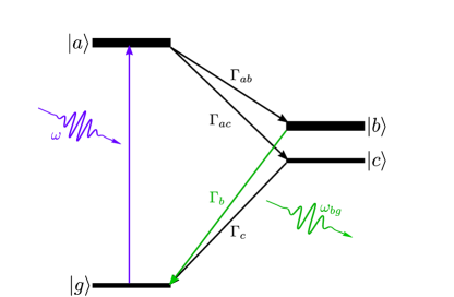
Figure 1: Energy-level diagram. Shown are the energy eigenstates of an atom and the electronic transitions relevant to the LSM.

Hereafter, we abandon the use of the overline to distinguish between perturbed and unperturbed atomic states. Despite the lack of an overline, quantum states should be interpreted as atomic states that have been perturbed by the static electric and magnetic fields $\mathbf{E}_{\mathrm{dc}}$ and $\mathbf{B}$, unless otherwise noted.

We consider a system in which atoms in the excited state undergo spontaneous decay to the lower states $|b\rangle$ and $|c\rangle$ with corresponding rates $\Gamma_{ab}$ and $\Gamma_{ac}=\Gamma_{a}-\Gamma_{ab}$, where $\Gamma_{a}$ is the natural linewidth of the state $|a\rangle$. A schematic of the relevant energy level structure is shown in Fig. 1. As atoms decay from $|b\rangle$ down to $|g\rangle$, they emit fluorescent light of frequency $\omega_{bg}$. The LSM involves both the simulation and measurement of the spectral lineshape of the $g\rightarrow a$ transition. In this context, the “spectral lineshape” refers to the probability of emission of fluorescent light of frequency $\omega_{bg}$ as a function of laser frequency $\omega$. Although polarizabilities $\alpha_{g}$ and $\alpha_{a}$ depend on $\omega$, we assume that they are effectively constant for $\omega\approx\omega_{ag}$. The LSM can be applied to any atomic system with the energy level structure shown in Fig. 1.

III Spectral lineshape

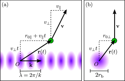
Figure 2: Parameters of atomic trajectory. The atom’s position $\mathbf{r}(t)$ and velocity $\mathbf{v}$ are shown for some time $t>0$ and have been projected onto two planes: (a) the plane formed by the vectors $\mathbf{k}$ and $\mathbf{v}$, where $\mathbf{k}$ is the wave-vector of the standing wave of light, and (b) the plane normal to $\mathbf{k}$ and containing the origin $O$. A contour plot of the spatial extent of the light intensity is shown for reference; white and purple indicate minimal (zero) and maximal intensity, respectively. Here $r_{0\parallel}$ and $r_{0\perp}$ correspond to the components of $\mathbf{r}(t)$ that are parallel and perpendicular to $\mathbf{k}$ when $t=0$.

The ac Stark shifts cause the resonant frequency of the $g\rightarrow a$ transition to shift as atoms travel through the standing wave. As a result, the spectral lineshape depends heavily on the details of the light field. Because the light field amplitude $E(\mathbf{r})$ is not spatially uniform [see Eq. (2) and the discussion thereafter], an atom with coordinate $\mathbf{r}(t)$ will experience a time-dependent electric field in its rest frame.

Assuming constant velocity, the atom’s position is $\mathbf{r}(t)=\mathbf{v}t+\mathbf{r}_{0}$ where $\mathbf{v}$ is the atomic velocity and $\mathbf{r}_{0}$ is the position of the atom when $t=0$. The origin $O$ is chosen to be at one of the nodes of the standing wave. A diagram of the geometry is shown in Fig. 2. The time-dependent field experienced by the atom is given by

$$E[\mathbf{r}(t)]=E_{0}\cos(kv_{\parallel}t+kr_{0\parallel})\,e^{-(v_{\perp}^{2}t^{2}+r_{0\perp}^{2})/r_{\mathrm{b}}^{2}},$$ (10)

where $E(\mathbf{r})$ is given by Eq. (2). Here $v_{\parallel}=\hat{\mathbf{k}}\cdot\mathbf{v}$ and $v_{\perp}=|\mathbf{v}-\hat{\mathbf{k}}\,v_{\parallel}|$ are the components of the velocity that are perpendicular and parallel to $\mathbf{k}$. Similarly, $r_{0\parallel}$ and $r_{0\perp}$ correspond to the perpendicular and parallel components of the position $\mathbf{r}_{0}$.

The total time dependence of the electric field in Eq. (1) is due to the fast oscillation of the light at frequency $\omega$ and the slow modulation of the amplitude with a frequency $kv_{\parallel}$. The amplitude modulation is additionally characterized by a temporal Gaussian envelope with a characteristic width $r_{\mathrm{b}}/v_{\perp}$, which is the amount of time an atom spends within the radius of the standing wave. We consider non-relativistic atoms for which the conditions $\omega\gg kv_{\parallel}$ and $\omega\gg v_{\perp}/r_{\mathrm{b}}$ are valid, and the optical oscillations are much faster than the modulation of the amplitude $E[\mathbf{r}(t)]$. In this case, the ac Stark shift is obtained by substituting Eq. (10) into Eq. (7).

III.1 Absorption profile

In order to gain a qualitative understanding of the physics, we make the simplifying assumption

$$E(t)\approx E_{0}\cos(kv_{\parallel}t).$$ (11)

In this case, the Stark shifts of the ground and excited states lead to the following shift of the resonant energy of the $g\rightarrow a$ transition:

$$\mathcal{E}_{\mathrm{ac}}(a)-\mathcal{E}_{\mathrm{ac}}(g)=-\frac{1}{2}\alpha_{ag}E_{0}^{2}\cos^{2}(kv_{\parallel}t),$$ (12)

where

$$\alpha_{ag}\equiv\alpha_{a}-\alpha_{g},$$ (13)

is the difference of the polarizabilities of the ground and excited states. From an atom’s perspective, this is equivalent to a polarizability-dependent frequency modulation of the two counterpropagting light fields. Thus, the features of the $g\rightarrow a$ lineshape can be understood by studying a related system: stationary atoms with fixed energy levels in the presence of two counter-propagating, frequency-modulated electric fields. In this subsection, we turn our attention to such a system.

The frequency-modulated electric fields have instantaneous frequencies $\omega_{+}$ and $\omega_{-}$ given by

$$\omega_{\pm}(t)=\omega\pm kv_{\parallel}+\omega_{\mathrm{m}}A_{\mathrm{m}}\cos(\omega_{\mathrm{m}}t),$$ (14)

where

$$\omega_{\mathrm{m}}\equiv 2kv_{\parallel}\quad\mathrm{and}\quad A_{\mathrm{m}}\equiv\frac{\alpha_{ag}E_{0}^{2}}{8\hbar kv_{\parallel}},$$ (15)

are the modulation frequency and modulation index, respectively. Equation (14) includes the term $\pm kv_{\parallel}$ which accounts for the Doppler shifts of the frequencies of the two counter-propagating waves. To derive Eq. (14), we used a trigonometric identity to write $\cos^{2}(kv_{\parallel}t)=(1/2)[1+\cos(2kv_{\parallel}t)]$ and we neglected the time-independent term because it can be interpreted as an overall shift of the optical frequency: $\omega\rightarrow\omega+\omega_{\mathrm{m}}A_{\mathrm{m}}$. The instantaneous frequency $\omega_{\pm}(t)$ is characteristic of a light field with a time-dependent phase Silver (1992). Such a field is given by

$$E_{\pm}=(1/2)E_{0}e^{i[(\omega\pm kv_{\parallel})t+A_{\mathrm{m}}\sin(\omega_{\mathrm{m}}t)]},$$ (16)

where the factor of 1/2 is included so that the total field, which is the sum of two traveling waves, has an amplitude of $E_{0}$. The effective field $E_{\pm}$ can be decomposed in the following way:

$$E_{\pm}=\sum_{n=-\infty}^{\infty}(1/2)E_{0}J_{n}(A_{\mathrm{m}})e^{i(\omega\pm kv_{\parallel}+n\omega_{\mathrm{m}})t},$$ (17)

where $J_{n}$ are Bessel functions of the first kind. Thus the effective field consists of a principal field ($n=0$) which oscillates at a frequency $\omega\pm kv_{\parallel}$, and infinitely many sidebands $(n\neq 0)$ which oscillate at frequencies $\omega\pm kv_{\parallel}+n\omega_{\mathrm{m}}$. The amplitude of the electric field of $n$th sideband is $(1/2)E_{0}J_{n}(A_{\mathrm{m}})$.

The total electric field $E_{\mathrm{tot}}$ seen by the atom is the sum of the two counter-propagating light fields. To add the fields, the summation index in Eq. (17) is changed from $n$ to $n+1$ and the field $E_{-}$ is expressed as

$$E_{-}=\sum_{n=-\infty}^{\infty}(1/2)E_{0}J_{n+1}(A_{\mathrm{m}})e^{i(\omega+kv_{\parallel}+n\omega_{\mathrm{m}})t},$$

where $-kv_{\parallel}+\omega_{\mathrm{m}}=+kv_{\parallel}$ because the modulation frequency $\omega_{\mathrm{m}}$ is exactly twice the Doppler shift. Hence the sidebands of the two counter-propagating waves overlap and the total field is given by

$$E_{\mathrm{tot}}=E_{+}+E_{-}=\sum_{n=-\infty}^{\infty}\mathcal{E}_{n}e^{i\omega_{n}t},$$ (18)

where

$$\mathcal{E}_{n}\equiv\frac{E_{0}}{2}[J_{n+1}+J_{n}]\quad\mathrm{and}\quad\omega_{n}\equiv\omega+kv_{\parallel}+2n\,kv_{\parallel}.$$ (19)

In particular, the first-order sidebands from one field correspond with the carrier of the other Stalnaker et al. (2006), resulting in an absorption profile with a polarizability-dependent distortion. The “absorption profile” is a plot of the transition rate as a function of $\omega$.

The rate of the $g\rightarrow a$ transition is given by

$$\mathcal{R}=\sum_{n=-\infty}^{\infty}\frac{2\pi}{\hbar^{2}}\left|d_{\mathrm{in}}\mathcal{E}_{n}\right|^{2}\frac{\Gamma_{a}/2\pi}{(\omega_{n}-\omega_{ag})^{2}+(\Gamma_{a}/2)^{2}}.$$ (20)

Equation (20) is valid in the weak excitation limit, that is, when the excitation rate $\mathcal{R}$ is much smaller than all other relevant rates. To derive Eq. (20), we neglected the interference of different harmonic components, e.g., $\mathcal{E}_{n}e^{i\omega_{n}t}$ and $\mathcal{E}_{n^{\prime}}e^{i\omega_{n^{\prime}}t}$. Such terms contribute small corrections to the transition rate which do not affect the qualitative behavior of the absorption profile. A plot of the absorption profile is given in Fig. 3. The single-atom absorption profile is clearly asymmetric about the atomic resonance ($\omega=\omega_{ag}$).

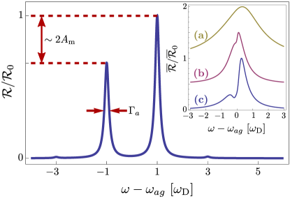
Figure 3: Absorption profile. Shown is a plot of the transition rate $\mathcal{R}$ as a function of the laser frequency $\omega$ for the case of a single atom with parallel speed $v_{\parallel}=\omega_{\mathrm{D}}/k$, where $\omega_{\mathrm{D}}$ is the Doppler broadening of the line. The transition rate is normalized by $\mathcal{R}_{0}$ to have a maximum value of unity. Here the modulation index satisfies $A_{\mathrm{m}}<0$. For $A_{\mathrm{m}}>0$, the peak on the left is taller than the peak on the right. In the insert, the average transition rate $\overline{\mathcal{R}}$ is shown in three cases: (a) the condition $\Gamma_{a}/4\ll\omega_{\mathrm{D}}$ is violated, (b) the condition $\hbar\omega_{\mathrm{D}}\lesssim|\alpha_{ag}|E_{0}^{2}$ is violated, and (c) both conditions in Eq. (22) are satisfied. To generate these curves, we made use of the approximation $k\approx k_{ag}$ which is valid in the near-resonant regime ($\omega\approx\omega_{ag}$).

For an ensemble of atoms, the absorption profile is obtained by averaging the transition rate (20) over the velocity distribution. The average rate is

$$\overline{\mathcal{R}}\equiv\int_{-\infty}^{\infty}\!\!\mathcal{R}(v_{\parallel})\,w_{\mathrm{L}}(v_{\parallel},v_{\mathrm{C}})\,dv_{\parallel},$$ (21)

where $w_{\mathrm{L}}(v_{\parallel},v_{\mathrm{C}})$ is the appropriate probability distribution for the parallel velocity $v_{\parallel}$, and $v_{\mathrm{C}}$ is a characteristic speed in the $\hat{\mathbf{k}}$ direction. A plot of the average transition rate is shown in the insert of Fig. 3. For the insert, $w_{\mathrm{L}}(v_{\parallel},v_{\mathrm{C}})$ is taken to be a Lorentzian distribution with a full-width at half the maximum value (FWHM) of $v_{\mathrm{C}}=\omega_{\mathrm{D}}/k$, where $\omega_{\mathrm{D}}$ is the overall Doppler broadening of the line. The resulting absorption profile is similar to experimentally observed lineshapes in Yb (Section IV).

The absorption profile exhibits a polarizability-dependent feature: a dip that separates the profile into two distinct peaks. The sign of the polarizability $\alpha_{ag}$ determines whether the peak on the left is larger or smaller than the peak on the right. The following conditions need to be met in order for the distortion to be observed:

$$\Gamma_{a}/4\ll\omega_{\mathrm{D}}\quad\mathrm{and}\quad\hbar\omega_{\mathrm{D}}\lesssim|\alpha_{ag}|E_{0}^{2}.$$ (22)

The former condition ensures that the sidebands of the FM waves can be resolved. The latter ensures that the amplitude of the first-order sidebands is not negligible compared to the amplitude of the carrier, that is, $A_{\mathrm{m}}\neq 0$ for $v_{\parallel}\approx v_{\mathrm{C}}$. If either $\omega_{\mathrm{D}}\lesssim\Gamma_{a}/4$ or $\hbar\omega_{\mathrm{D}}\gg|\alpha_{ag}|E_{0}^{2}$, then the asymmetric distortion will be suppressed, as can be seen in the insert of Fig. 3. In this case, the methods described here cannot be used to measure the polarizability $\alpha_{ag}$. However, the LSM can still be used to measure $\alpha_{ag}$ in the absence of the distortion by comparing displacements of the central peak of the lineshape.

By omitting the Gaussian envelope $\exp(-v_{\perp}^{2}t^{2}/r_{\mathrm{b}}^{2})$ in Eq. (11), we neglect effects of the atom’s finite transit time, such as broadening of the spectral line Demtröder (2003). Nonetheless, the transit time must satisfy the following restrictions:

$$v_{\perp}/r_{\mathrm{b}}\lesssim d_{\mathrm{in}}E_{0}/\hbar\quad\mathrm{and}\quad v_{\perp}/r_{\mathrm{b}}\ll\omega_{\mathrm{D}},$$ (23)

where $d_{\mathrm{in}}E_{0}/\hbar$ is the Rabi frequency of the $g\rightarrow a$ transition. The former condition represents a system in which atoms have enough time to undergo excitation to the upper state $|a\rangle$, as will be discussed in Section III.2. The latter condition ensures that the Doppler broadening is sufficiently large that most atoms travel through many nodes and antinodes of the standing wave during their transit.

Although the absorption profile provides a satisfactory illustration of the physics, it cannot be used to measure the ac polarizabilities. The transition rate presented in Eq. (20) is valid only in the weak excitation limit and therefore cannot account for saturation effects. Moreover, Eq. (20) does not properly take into account interference of different probability amplitudes, nor does it include finite transit-time effects. A more complete picture is required to generate a theoretical lineshape that can be fitted to experimental data. Such a picture is achieved by the following model.

III.2 Fluorescence probability

Hereafter, we return our attention to the original system: moving atoms illuminated by light with a fixed frequency $\omega$. The spectral lineshape of the $g\rightarrow a$ transition is modeled by computing the probability of emission of fluorescent light of frequency $\omega_{bg}$ as a function of laser frequency $\omega$. The computation involves three steps. First, the time-dependent population $\rho_{bb}$ of the state $|b\rangle$ is computed by numerically solving the optical Bloch equations (OBE) for the case of atoms traveling through a non-uniform field (see Fig. 2). Second, the probability of fluorescence $\mathcal{F}$ is determined by integrating the time-dependent decay rate $\Gamma_{b}\rho_{bb}$ with respect to time. Finally, the average fluorescence probability $\overline{\mathcal{F}}$ is computed by taking a weighted average of $\mathcal{F}$ with respect to the atomic velocity $\mathbf{v}$ and the offset $\mathbf{r}_{0}$.

Although the LSM can be used in conjunction with any atomic source, our model makes use of distributions that are appropriate for a collimated beam of thermal atoms traveling in a direction that is orthogonal to the standing wave. In this case, $v_{\perp}$ represents the component of the atom’s velocity along the atomic beam, and $v_{\parallel}/v_{\perp}$ represents the angular spread of the beam. The corresponding velocity distribution is

$$w(\mathbf{v})=w_{\mathrm{T}}(v_{\perp},v_{\mathrm{T}})\,w_{\mathrm{L}}(v_{\parallel},v_{\mathrm{C}}),$$ (24)

where

$$w_{\mathrm{T}}(v_{\perp},v_{\mathrm{T}})=2(v_{\perp}^{3}/v_{\mathrm{T}}^{4})e^{-(v_{\perp}/v_{\mathrm{T}})^{2}},$$ (25)

is the distribution of velocities appropriate for thermal atoms escaping from a hole, and $w_{\mathrm{L}}(v_{\parallel},v_{\mathrm{C}})$ is the velocity distribution appropriate for a collimated atomic beam. Here $v_{\mathrm{T}}=\sqrt{2k_{B}T/M}$ is the thermal speed of the atom, $T$ is the temperature of the oven, $M$ is the atom’s mass, $k_{B}$ is Boltzmann’s constant, and $v_{\mathrm{C}}$ is the characteristic speed determined by the atomic-beam collimator. To model the effects of a vane collimator, we approximate the spread of parallel velocities by a Lorentzian distribution with a FWHM of $v_{\mathrm{C}}=\omega_{\mathrm{D}}/k$, where $\omega_{\mathrm{D}}$ is the overall Doppler broadening of the line.

In the following model, we use dimensionless parameters. Dimensionless parameters ease computation, and potentially facilitate the application of the model to several different atomic systems. Throughout, we make the approximation $k\approx k_{ag}$ which is valid in the near-resonant regime ($\omega\approx\omega_{ag}$).

Time is measured in units $1/\Gamma_{a}$. We define the dimensionless time $\tau\equiv\Gamma_{a}\,t$ and decay rates $G_{b}\equiv\Gamma_{b}/\Gamma_{a}$, $G_{c}\equiv\Gamma_{c}/\Gamma_{a}$, $G_{ab}=\Gamma_{ab}/\Gamma_{a}$, and $G_{ac}=1-G_{ab}$. We further define the dimensionless perpendicular and parallel velocities $u_{\perp}\equiv v_{\perp}/v_{\mathrm{T}}$ and $u_{\parallel}\equiv v_{\parallel}/v_{\mathrm{C}}$, and the dimensionless perpendicular and parallel offsets $\xi\equiv r_{0\perp}/r_{\mathrm{b}}$ and $\varphi\equiv kr_{0\parallel}$, respectively.

Consistent with the discussion in Section III.1, we introduce the following dimensionless parameters: the saturation parameter $S_{0}$, characteristic modulation index $S_{1}$, and Doppler parameter $S_{2}$, defined by

$$S_{0} \equiv\left[d_{\mathrm{in}}E_{0}/(\hbar\Gamma_{a})\right]^{2},$$ (26)

$$S_{1} \equiv\alpha_{ag}E_{0}^{2}/(8\hbar\omega_{\mathrm{D}}),$$ (27)

and

$$S_{2}\equiv 2\omega_{\mathrm{D}}/\Gamma_{a},$$ (28)

respectively. We define an additional parameter $S_{3}$ by

$$S_{3}\equiv v_{\mathrm{T}}/(r_{\mathrm{b}}\Gamma_{a}).$$ (29)

Note that $r_{\mathrm{b}}/v_{\perp}$ is the time that an atom spends within the radius of the light field and hence $1/(S_{3}\,u_{\perp})$ represents the dimensionless transit time.

In terms of the dimensionless parameters, the conditions presented in expressions (22) reduce to $S_{2}\gg 1/2$ and $|S_{1}|\gtrsim 1/8$. When either of these conditions is violated, the characteristic dip in the lineshape is suppressed, as can be seen in Fig. 4. Likewise, conditions (23) reduce to $S_{3}\lesssim\sqrt{S_{0}}$ and $S_{3}\ll(1/2)S_{2}$. Whereas the absorption profile discussed in Section III.1 was valid only in the weak excitation limit $(S_{0}\ll 1)$, the model of the fluorescence can accommodate large saturation parameters.

Let $\rho_{nm}$ be the elements of the density matrix in the atom’s rest frame for states $n,m\in\{g,a,b,c\}$. We assume that the rotating wave approximation holds and dynamic interactions between states other than $|g\rangle$ and $|a\rangle$ can be neglected. In this case, the dimensionless optical Bloch equations (OBE) for the configuration shown in Fig. 1 are Loudon (2000)

$$\dot{\rho}_{aa} =-\frac{i}{2}\Omega(\rho_{ag}-\rho_{ga})-\rho_{aa},$$ (30a)

$$\dot{\rho}_{ag} =+\frac{i}{2}\Omega(\rho_{gg}-\rho_{aa})-\frac{1}{2}(1-2i\Delta)\rho_{ag},$$ (30b)

$$\dot{\rho}_{bb} =-G_{b}\rho_{bb}+G_{ab}\rho_{aa},$$ (30c)

$$\dot{\rho}_{cc} =-G_{c}\rho_{cc}+G_{ac}\rho_{aa},$$ (30d)

where $\dot{\rho}_{nm}=d(\rho_{nm})/d\tau$. The remaining density matrix elements $\rho_{gg}$ and $\rho_{ga}$ are determined from $\sum_{n}\rho_{nn}=1$ and $\rho_{ga}=\rho_{ag}^{\ast}$. Here

$$\Omega\equiv\frac{1}{\Gamma_{a}}\left[\frac{\langle a|\mathbf{d}\cdot\boldsymbol{\epsilon}|g\rangle E(t)}{\hbar}\right]=\sqrt{S_{0}}\,f(\boldsymbol{\xi},\mathbf{u}),$$ (31)

is the Rabi frequency,

$$\Delta\equiv\frac{1}{\Gamma_{a}}\left[\omega-\frac{\mathcal{E}(a)-\mathcal{E}(g)}{\hbar}\right]=\delta+2S_{1}S_{2}\,f(\boldsymbol{\xi},\mathbf{u})^{2},$$ (32)

is the detuning of the laser light from the resonance, $\delta\equiv(\omega-\omega_{ag})/\Gamma_{a}$, and the function $f(\boldsymbol{\xi},\mathbf{u})$ is defined by

$$f(\boldsymbol{\xi},\mathbf{u})\equiv\cos[(S_{2}/2)u_{\parallel}\tau+\varphi]e^{-[(S_{3}u_{\perp}\tau)^{2}+\xi^{2}]},$$ (33)

where $\boldsymbol{\xi}=(\varphi,\xi)$ and $\mathbf{u}=(u_{\parallel},u_{\perp})$. We further assume that all atoms initially occupy the ground state.

The probability that an atom will emit fluorescent light of frequency $\omega_{bg}$ in a time interval $[\tau_{\mathrm{i}},\tau_{\mathrm{f}}]$ is given by

$$\mathcal{F}=\int_{\tau_{\mathrm{i}}}^{\tau_{\mathrm{f}}}G_{b}\,\rho_{bb}(\tau)\,d\tau,$$ (34)

where $G_{b}\,\rho_{bb}(\tau)$ is the time-dependent rate of the $b\rightarrow g$ decay. The choice of integration interval $[\tau_{\mathrm{i}},\tau_{\mathrm{f}}]$ depends on both the transit time and the characteristic time of the fluorescent decay after the atoms leave the light field. In the case where the $a\rightarrow b\rightarrow g$ decay time is shorter than the transit time, it is appropriate to define the integration limits by $-\tau_{\mathrm{i}}=\tau_{\mathrm{f}}=3/(S_{3}\,u_{\perp})$. The factor of 3 ensures that the atom is “far” from the standing wave at the integration limits. To model a system with slower decays, the integration limit $\tau_{\mathrm{f}}$ must be extended.

The fluorescence probability depends on the parameters of the atomic trajectory, that is, $\mathcal{F}=\mathcal{F}(\boldsymbol{\xi},\mathbf{u})$. We define the average probability of fluorescence by

$$\overline{\mathcal{F}}=\iint\mathcal{F}(\boldsymbol{\xi},\mathbf{u})\,w(\boldsymbol{\xi},\mathbf{u})\,d\boldsymbol{\xi}\,d\mathbf{u},$$ (35)

where $w(\boldsymbol{\xi},\mathbf{u})$ is the probability distribution associated with the atom’s initial position and velocity. In our model, we assume $w(\boldsymbol{\xi},\mathbf{u})=w_{1}(\boldsymbol{\xi})\,w_{2}(\mathbf{u})$, where the distribution $w_{1}$ is a uniform distribution over the intervals $\xi\in[-3,3]$ and $\varphi\in[-\pi,\pi]$. The finite integration limits are justified by the following properties of the system: First, the amplitude of the standing wave drops to less than 0.01% of its maximum value when $|\xi|>3$. Therefore, atoms will only pass through the light if $|\xi|\lesssim 3$. Second, $\varphi$ constitutes a phase shift of the electric field which is unique only for $\varphi\in[-\pi,\pi]$. Consistent with Eqs. (24) and (25), the velocity distribution satisfies $w_{2}(\mathbf{u})=w_{\mathrm{T}}(u_{\perp},1)w_{\mathrm{L}}(u_{\parallel},1)$, where $w_{\mathrm{T}}(u_{\perp},1)$ is the velocity distribution for atoms escaping from a hole with unit thermal speed, and $w_{\mathrm{L}}(u_{\parallel},1)$ is a Lorentzian distribution with FWHM of 1.

Figure 4: Results of simulation. The simulated lineshape $\overline{\mathcal{F}}(\delta)$ is shown for two different values each of the modulation index $S_{1}$ and the Doppler parameter $S_{2}$, as indicated by the insert: (a) the condition $S_{2}\gg 1/2$ is violated, (b) the condition $|S_{1}|\gtrsim 1/8$ is violated, and (c) both conditions are satisfied. For each curve, the saturation parameter is $S_{0}=1.0$. The lineshapes are normalized by the maximum peak height $\overline{\mathcal{F}}_{0}$. To ease comparison, the middle and top curves are shifted vertically by 0.7 and 1.0, respectively.

The fluorescence probability is a function of the detuning $\delta$ from the atomic resonance, that is,

$$\overline{\mathcal{F}}=\overline{\mathcal{F}}(\delta;\mathbf{S},\mathbf{G}),$$ (36)

where $\mathbf{S}\equiv(S_{0},S_{1},S_{2},S_{3})$ and $\mathbf{G}\equiv(G_{ab},G_{b},G_{c})$ are parameters. We refer to a plot of $\overline{\mathcal{F}}(\delta;\mathbf{S},\mathbf{G})$ as a function of $\delta$ as the “simulated lineshape” of the $g\rightarrow a$ transition. Three such plots are shown in Fig. 4. In Fig. 4, curves (a) and (b) demonstrate the suppression of the polarizability-dependent distortion when either the Doppler parameter $S_{2}$ or the modulation index $S_{1}$ is too small. The distortion is most pronounced in curve (c), for which $S_{2}\gg 1/2$ and $|S_{1}|\gtrsim 1/8$. The simulated lineshapes in Fig. 4 are qualitatively similar to the absorption profiles in the insert of Fig. 3, as expected.

III.3 Numerical procedure

The numerical procedures described here are valid for a variety of atomic species. However, the simulations were performed with parameter values appropriate for the Yb system described in Section IV.

We used a stiffly stable Rosenback method Press et al. (2007) to numerically solve a system of equations related to Eqs. (30) and (34), with $-\tau_{\mathrm{i}}=\tau_{\mathrm{f}}=3/(S_{3}\,u_{\perp})$. This system of equations is described in Appendix B. The Rosenback method involves two tolerances–denoted atol and rtol in Ref. Press et al. (2007)–which were both set to $10^{-5}$. The multi-dimensional integral in Eq. (35) was computed using an adaptive Monte Carlo routine Press et al. (2007). In our implementation, the integration routine involves $10^{5}$ evaluations of the integrand. For various values of $\mathbf{S}$, the average estimated error was less than 1% of the value of the integral.

For computational purposes, we restricted the integration to the following finite domain: $\xi\in[-3,3]$, $\varphi\in[-\pi,\pi]$, $u_{\perp}\in[0,3]$, and $u_{\parallel}\in[-6,6]$. The subdomains for $\xi$ and $\varphi$ were discussed after Eq. (35). The finite integration subdomains for $u_{\parallel}$ and $u_{\perp}$ are justified as follows: Atoms with a large parallel speed $|u_{\parallel}|$ experience a Doppler shift that is much larger than the characteristic Doppler broadening of the spectral line. Such atoms only contribute to the wings of the lineshape, where $|\delta|$ is large and the probability of fluorescence is very small. Moreover, for a Lorentzian velocity distribution with unit FWHM, $|u_{\parallel}|\leq 6$ for about 95% of atoms.

On the other hand, atoms with a perpendicular speed that satisfies $u_{\perp}\gg\sqrt{S_{0}}/S_{3}$ are moving so fast that the transit time is much smaller than the inverse Rabi frequency. Such atoms do not spend enough time in the light field for the $g\rightarrow a$ transition to be realized. Since most atoms travel at or near the thermal speed $u_{\perp}=1$, the condition $\sqrt{S_{0}}/S_{3}\gtrsim 1$ represents a system in which most atoms have enough time to interact with the light. We assume that atoms with speed $u_{\perp}>3$ do not contribute significantly to the lineshape. Note that $u_{\perp}>3$ for only about 0.1% of atoms. Finally, we ignore counterflow of atoms in the atomic beam by requiring $u_{\perp}\geq 0$.

For fixed $\mathbf{G}=(0.35,0.45,0)$ and $S_{3}=0.53$, we computed the average fluorescence $\overline{\mathcal{F}}(\delta;\mathbf{S},\mathbf{G})$ for 100 discrete values of $\delta\in[\delta_{-},\delta_{+}]$, and various discrete values of $S_{0}\in[0.1,10]$, $S_{1}\in[0.01,1]$, and $S_{2}\in[1,100]$. Here $\delta_{\pm}\equiv 2S_{1}S_{2}\pm 3[(1/2)S_{2}+G_{b}+1]$. The results were interpolated using cubic splines to approximate the continuous function $\overline{\mathcal{F}}(\delta;\mathbf{S},\mathbf{G})$. Three curves which are typical of those produced by this procedure are presented in Fig. 4.

The LSM involves fitting the simulated curve $\overline{\mathcal{F}}(\delta;\mathbf{S},\mathbf{G})$ to the observed lineshape to determine best-fit values of $S_{0}$, $S_{1}$, and $S_{2}$. From the best-fit values, the following three quantities can be calculated: the polarizability difference $\alpha_{ag}$, the circulating power $P$ of the standing wave, and the Doppler broadening $\omega_{\mathrm{D}}$ of the $g\rightarrow a$ transition which are given by

$$\alpha_{ag} =\left[\frac{4\,d_{\mathrm{in}}^{2}}{\hbar\,\Gamma_{a}}\right]\times S_{1}S_{2}/S_{0},$$ (37)

$$P =\left[\frac{1}{16}\pi\,r_{\mathrm{b}}^{2}\,c\,\epsilon_{0}\frac{\hbar^{2}\,\Gamma_{a}^{2}}{d_{\mathrm{in}}^{2}}\right]\times S_{0},$$ (38)

and

$$\omega_{\mathrm{D}}=(\Gamma_{a}/2)\times S_{2},$$ (39)

respectively. Here $\epsilon_{0}$ is the permittivity of free space. The present implementation of the LSM uses Mathematica’s nonlinear regression routine to determine the best-fit values of $S_{0}$, $S_{1}$, and $S_{2}$. Alternatively, Eq. (38) can be solved for $d_{\mathrm{in}}$ in terms of $P$ and $S_{0}$. Thus the LSM can also be used to measure the induced dipole moment when the power is known, as was done in the previous application of the LSM Stalnaker et al. (2006).

The treatment of systematic errors and statistical uncertainties is straightforward. In Eq. (37), for instance, the uncertainty in the dimensionful quantity $d_{\mathrm{in}}^{2}/(\hbar\Gamma_{a})$ is due solely to systematic effects, whereas the uncertainty in the term $S_{1}S_{2}/S_{0}$ arises from statistical uncertainties in both the observed signal and the fitting algorithm. The total uncertainty of the quantity $\alpha_{ag}$ is obtained by adding these independent uncertainties in quadrature. If the signal-to-noise ratio (SNR) of the observed lineshape is sufficiently high, then the error of the measurement of $\alpha_{ag}$ will be dominated by the uncertainties of the known quantities $d_{\mathrm{in}}$ and $\Gamma_{a}$.

IV Application to Ytterbium

The electronic structure of Yb is shown in Fig. 5. The low-lying energy eigenstates of Yb match the structure shown in Fig. 1 under the following mapping: $|g\rangle=|\mathrm{{}^{1}S_{0}}\rangle$, $|a\rangle=|\mathrm{{}^{3}D_{1}}\rangle$, $|b\rangle=|\mathrm{{}^{3}P_{1}}\rangle$, and $|c\rangle=|\mathrm{{}^{3}P_{0}}\rangle$. Therefore, the LSM can be used to measure the difference in ac polarizabilities of the upper state $|\mathrm{{}^{3}D_{1}}\rangle$ and the ground state $|\mathrm{{}^{1}S_{0}}\rangle$ at 408 nm by analyzing the lineshape of the 408-nm $\mathrm{{}^{1}S_{0}}\rightarrow\mathrm{{}^{3}D_{1}}$ transition. In this case, the lineshape is measured by observing the 556-nm fluorescence of the $\mathrm{{}^{3}P_{1}}\rightarrow\mathrm{{}^{1}S_{0}}$ decay. The intermediate state $|\mathrm{{}^{3}P_{0}}\rangle$ is metastable and hence $\Gamma_{c}\approx 0$.

There is an additional decay of $|\mathrm{{}^{3}D_{1}}\rangle$ to the metastable state $|\mathrm{{}^{3}P_{2}}\rangle$, which is not shown in Fig. 1. The state $|c\rangle$ can represent multiple metastable states, including both $|\mathrm{{}^{3}P_{1}}\rangle$ and $|\mathrm{{}^{3}P_{2}}\rangle$. In this interpretation, $\Gamma_{ac}$ is the rate of decay of $|\mathrm{{}^{3}D_{1}}\rangle$ to all metastable states.

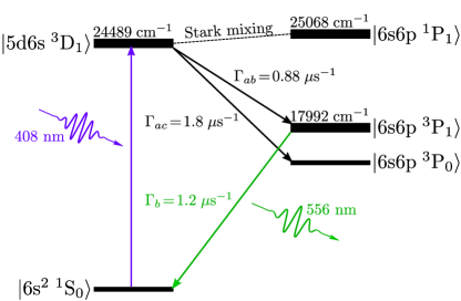
Figure 5: Ytterbium energy levels. Shown are the low-lying energy eigenstates of Yb and the electronic transitions relevant to the polarizability experiment.

The highly forbidden $\mathrm{{}^{1}S_{0}}\rightarrow\mathrm{{}^{3}D_{1}}$ transition is induced by the Stark mixing technique. This technique involves the application of a static, uniform electric field $\mathbf{E}_{\mathrm{dc}}$ which mixes the upper state $|\mathrm{{}^{3}D_{1}}\rangle$ with opposite-parity states, predominantly the $|\mathrm{{}^{1}P_{1}}\rangle$ state. The effective dipole moment $d_{\mathrm{in}}$ associated with the Stark-induced transition is given by Stalnaker et al. (2006)

$$d_{\mathrm{in}}=\beta_{ag}|(\mathbf{E}_{\mathrm{dc}}\times\boldsymbol{\epsilon})^{(1)}_{-M_{a}}|,$$ (40)

where $\beta_{ag}=2.18(10)\times 10^{-8}\;e\cdot a_{0}\cdot(\mathrm{V}/\mathrm{cm})^{-1}$ is the vector transition polarizability of the $\mathrm{{}^{1}S_{0}}\rightarrow\mathrm{{}^{3}D_{1}}$ transition, $e$ is the elementary charge, $a_{0}$ is the Bohr radius, and $(\mathbf{E}_{\mathrm{dc}}\times\boldsymbol{\epsilon})^{(1)}$ is a spherical tensor of rank one. Here $M_{a}$ is the magnetic quantum number of the $|\mathrm{{}^{3}D_{1}}\rangle$ state.

Because the angular momentum of the ground state $|\mathrm{{}^{1}S_{0}}\rangle$ is $J_{g}=0$, only the scalar term in Eq. (9) contributes to the polarizability of $|\mathrm{{}^{1}S_{0}}\rangle$. That is, $\alpha_{g}=\alpha_{0}(\mathrm{{}^{1}S_{0}})$ and so $\alpha_{g}$ is independent of the geometry of the applied fields. Hence the dependence of $\alpha_{ag}$ on the field geometry is due entirely to the vector and tensor polarizabilities $\alpha_{1}(\mathrm{{}^{3}D_{1}})$ and $\alpha_{2}(\mathrm{{}^{3}D_{1}})$ of the excited state $|\mathrm{{}^{3}D_{1}}\rangle$. In this case, the LSM is sensitive to the difference of the scalar polarizabilities of the ground and excited states. However, the vector and tensor polarizabilities of the excited state can be measured unambiguously by varying the polarization of the standing wave.

A recent calculation Derevianko and Dzuba of the polarizability of the ground state $|\mathrm{{}^{1}S_{0}}\rangle$ at 408 nm yielded

$$\alpha_{0}(\mathrm{{}^{1}S_{0}})=0.218(11)\;\mathrm{Hz}\cdot\mathrm{(V/cm)^{-2}}.$$ (41)

Calculations of the polarizability $|\mathrm{{}^{3}D_{1}}\rangle$ at 408 nm are complicated by the potential existence of odd-parity eigenstates with energy close to twice the energy of a 408-nm photon. Such states could lead to a resonantly enhanced polarizability of the $\mathrm{{}^{3}D_{1}}$ state. The energy spectrum in this region (which is below the ionization limit) is very dense due to the excitation of $4f$ orbitals. The knowledge of the energy spectrum is far from complete in this region. This provides one of the motivations for determining the polarizabilities experimentally.

The first implementation of the LSM Stalnaker et al. (2006) was used to measure the quantity

$$\alpha_{ag}^{\mathrm{I}}=-0.312(34)\;\mathrm{Hz}\cdot\mathrm{(V/cm)^{-2}},$$ (42)

were $\alpha_{ag}^{\mathrm{I}}=\alpha_{2}(\mathrm{{}^{3}D_{1}})+\alpha_{0}(\mathrm{{}^{3}D_{1}})-\alpha_{0}(\mathrm{{}^{1}S_{0}})$. Here the superscript “I” is introduced to distinguish this measurement from the results of the present work. To determine the tensor contribution $\alpha_{2}(\mathrm{{}^{3}D_{1}})$ unambiguously requires a second measurement of a different combination of scalar and tensor polarizabilities. This is accomplished in the present work by the application of a dc electric field that is parallel to the standing wave (Fig. 6), whereas the previous measurement was performed with a dc field that was perpendicular to the standing wave. In addition, the current experiment includes a strong magnetic field not present in the previous case. The magnetic field makes possible the measurement of the vector polarizability, as discussed in Section V.

IV.1 Experimental apparatus and field geometry

The details of the experimental apparatus were reported elsewhere Tsigutkin et al. (2010), and only a brief description is provided here. A schematic of the setup is shown in Fig. 6. A beam of Yb atoms is produced by a stainless-steel oven loaded with Yb metal, operating at 500 ^∘C. The oven is outfitted with a multislit nozzle, and there is an external vane collimator reducing the spread of the atomic beam in the $z$-direction. Downstream from the collimator, atoms enter a region with three external fields: a uniform, static magnetic field $\mathbf{B}$; a uniform, static electric field $\mathbf{E}_{\mathrm{dc}}$; and a non-uniform, dynamic electric field $\mathbf{E}(\mathbf{r},t)$.

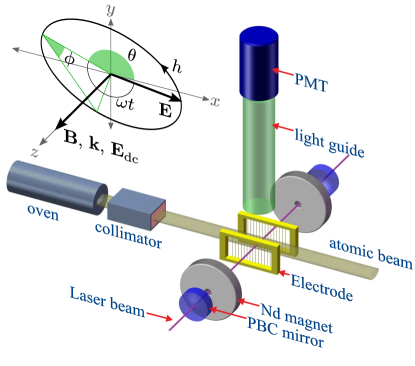
Figure 6: Experimental apparatus. A collimated beam of ytterbium atoms interacts with a standing wave of light in the presence of dc electric and magnetic fields. The light is resonant with the 408-nm $\mathrm{{}^{1}S_{0}}\rightarrow\mathrm{{}^{3}D_{1}}$ transition, and the 556-nm fluorescence is detected by the photomultiplier tube (PMT). The neodymium (Nd) magnets are axially magnetized in the $z$-direction. The standing wave is generated in a power buildup cavity (PBC). With the exception of the PMT, the apparatus is contained in a vacuum chamber.

The magnetic field $\mathbf{B}$ is generated by a pair of axially magnetized neodymium (Nd) magnets. These magnets produce a field with sufficient strength (more than 50 G) to completely isolate the Zeeman sublevels of the upper state $|\mathrm{{}^{3}D_{1}}\rangle$. The electric field $\mathbf{E}_{\mathrm{dc}}$ is generated by two wire-frame electrodes separated by 2 cm. The ac electric field $\mathbf{E}(\mathbf{r},t)$ is due to standing-wave light at the transition wavelength of 408.346 nm in vacuum, which is produced by doubling the frequency of the output of a Ti:sapphire laser (Coherent 899). About 7 mW of 408-nm light is coupled into a power buildup cavity (PBC) with finesse of approximately 15,000. The PBC is an asymmetric cavity with a flat input mirror and a curved back mirror with a 50-cm radius of curvature. The separation between the mirrors is 22 cm.

Fluorescent light with a wavelength of 556 nm is collected with a light guide and detected with a photomultiplier tube (PMT). With the exception of the PMT, the entire apparatus is contained within a vacuum chamber with a residual gas pressure of $3\times 10^{-6}$ Torr.

As can be seen in Fig. 6, the fields $\mathbf{B}$ and $\mathbf{E}_{\mathrm{dc}}$ point in the $\hat{\mathbf{z}}$ direction. Likewise, the standing wave is oriented along the $z$-axis. The light field $\mathbf{E}(\mathbf{r},t)$ lies in the $xy$-plane. For this geometry, the transition to the upper state $|\mathrm{{}^{3}D_{1}};M_{a}=0\rangle$ is suppressed.

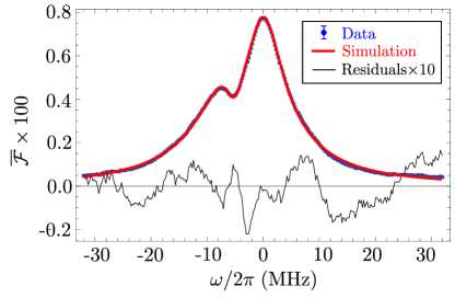
Figure 7: Results of fitting program. Shown is a comparison of the observed and the simulated lineshapes of the $\mathrm{{}^{1}S_{0}}\rightarrow\mathrm{{}^{3}D_{1}}$ transition. The data correspond to Run 3 in Table 1. Also shown are the residuals, magnified by a factor of 10. The residuals are the difference of the data and the simulation.

The polarization of the light field is of the form $\boldsymbol{\epsilon}=\epsilon_{x}\,\hat{\mathbf{x}}+\epsilon_{y}\,\hat{\mathbf{y}}$, where $|\epsilon_{x}|^{2}+|\epsilon_{y}|^{2}=1$. To further characterize the polarization, we introduce three parameters: polarization angle $\theta$, degree of ellipticity $\phi$, and handedness $h$, which are given by Auzinsh et al. (2010)

$$\tan 2\theta =2\,\mathrm{Re}(\epsilon_{x}\epsilon_{y}^{\ast})/(|\epsilon_{x}|^{2}-|\epsilon_{y}|^{2}),$$ (43)

$$\sin 2\phi =2\,|\mathrm{Im}(\epsilon_{x}\epsilon_{y}^{\ast})|=|i(\boldsymbol{\epsilon}\times\boldsymbol{\epsilon}^{\ast})\cdot\hat{\mathbf{z}}|,$$ (44)

and

$$h=-\mathrm{sgn}[i(\boldsymbol{\epsilon}\times\boldsymbol{\epsilon}^{\ast})\cdot\hat{\mathbf{z}}].$$ (45)

Linearly, circularly, and elliptically polarized light are described by $\phi=0$, $\phi=\pi/4$, and $0<\phi<\pi/4$, respectively. The sense of rotation is determined by $h$: left and right-handed polarizations correspond to $h=+1$ and $h=-1$, respectively. Substituting $\mathbf{E}_{\mathrm{dc}}=E_{\mathrm{dc}}\,\hat{\mathbf{z}}$ and $\boldsymbol{\epsilon}=\epsilon_{x}\,\hat{\mathbf{x}}+\epsilon_{y}\,\hat{\mathbf{y}}$ into Eqs. (40) and (9) yields

$$d_{\mathrm{in}}=\beta_{ag}E_{\mathrm{dc}}\sqrt{(1/2)[1+hM_{a}\sin(2\phi)]},$$ (46)

and

$$\alpha_{a}=\alpha_{0}(\mathrm{{}^{3}D_{1}})-hM_{a}\sin(2\phi)\alpha_{1}(\mathrm{{}^{3}D_{1}})-\frac{1}{2}\alpha_{2}(\mathrm{{}^{3}D_{1}}),$$ (47)

for $M_{a}=\pm 1$. Here we have used Eqs. (44) and (45) to eliminate $\epsilon_{x}$ and $\epsilon_{y}$ in favor of the degree of ellipticity $\phi$ and the handedness $h$. For this geometry, both $d_{\mathrm{in}}$ and $\alpha_{a}$ are independent of the polarization angle $\theta$.

According to the geometry in Fig. 6, the component of the atom’s velocity that is perpendicular to the standing wave is $v_{\perp}=(v_{x}^{2}+v_{y}^{2})^{1/2}$. The output of the oven is about 6 mm in the $y$-direction, and is located more than 20 cm away from the standing wave. In order for an atom to pass through the standing wave, its velocity components must satisfy $|v_{y}/v_{x}|\leq 0.015$. Therefore, the approximation $v_{\perp}=v_{x}$ is valid and the use of the thermal distribution given in Eq. (25) is justified. However, for a high-precision measurement, the effect of this approximation needs to be investigated.

IV.2 Data analysis

Table 1: Summary of results. The uncertainty in the fitted parameters is the asymptotic standard error returned by the fitting algorithm.

Run	$c_{0}\!\cdot\!10^{2}$	$c_{1}\!\cdot\!10^{2}$	$S_{0}$	$S_{1}$	$S_{2}$	$S_{1}S_{2}/S_{0}$
1	5.1(1)	5.5(4)	2.83(17)	-0.208(3)	34(1.1)	-2.53(16)
2	5.0(1)	3.2(3)	2.76(16)	-0.215(3)	30(1.1)	-2.33(17)
3	5.4(1)	7.0(3)	2.68(12)	-0.187(2)	34(1.0)	-2.35(13)
4	5.0(1)	4.7(3)	2.56(17)	-0.195(3)	29(1.1)	-2.22(17)
Avg.:			2.70(7)	-0.199(1)	31.8(5)	-2.36(8)

The data were acquired over four separate experiments (runs). During each run, approximately 2000 lineshapes were recorded at a rate of about 100 ms per lineshape and an average lineshape was computed. This procedure resulted in 4 lineshapes, each with an effective integration time of about 200 s. A typical lineshape is shown in Fig. 7. After fitting the theoretical model to the data, the statistical uncertainties of each run were scaled to give a reduced $\chi^{2}$ of unity. The scale factor varied between 4.0 and 4.7 depending on the run. The resulting error bars are shown in the figure. The relatively large scale factor indicates that the accuracy of the fit is dominated by either systematic distortion of the profile during the scan, or profile features that are neglected in the theoretical model, but not by the statistical uncertainty of the signal.

In the present experiment, the oven temperature was $T=500(50)\;{}^{\circ}\mathrm{C}$ and the magnitude of the dc electric field was $E_{\mathrm{dc}}=4.24(6)$ kV/cm. The atoms intersect the standing wave in the middle of the PBC where the radius of the light beam is $r_{\mathrm{b}}=196(5)\;\mathrm{\mu m}$. We used linearly polarized light with $\phi=0(1)^{\circ}$. Then Eqs. (37) through (39) become

$$\alpha_{ag}^{\mathrm{II}} =[0.0668(86)\;\mathrm{Hz\cdot(V/cm)^{-2}}]\times S_{1}S_{2}/S_{0},$$ (48)

$$P =[5.02(98)\;\mathrm{W}]\times S_{0},$$ (49)

and

$$\omega_{\mathrm{D}}=[2\pi\times 0.209(17)\;\mathrm{MHz}]\times S_{2},$$ (50)

where $\alpha_{ag}^{\mathrm{II}}=\alpha_{0}(\mathrm{{}^{3}D_{1}})-(1/2)\alpha_{2}(\mathrm{{}^{3}D_{1}})-\alpha_{0}(\mathrm{{}^{1}S_{0}})$. Here the superscript “II” is used to distinguish the results of the present work from the previous measurement. The dimensionless decay rates are $G_{ab}=0.35(4)$, $G_{b}=0.45(4)$, and $G_{c}=0$, and the parameter $S_{3}$ is given by $S_{3}=0.53(5)$.

As part of our analysis, we normalized the observed and simulated lineshapes by their maximum values. In addition, we introduced two calibration parameters to the simulated curve:

$$\overline{\mathcal{F}}(x;\mathbf{S},\mathbf{G},\mathbf{c})=(1+c_{0})\overline{\mathcal{F}}((1-c_{1})x;\mathbf{S},\mathbf{G})-c_{0},$$ (51)

where $\mathbf{c}=(c_{0},c_{1})$. Here $c_{0}$ accounts for the background of the observed signal. The parameter $c_{1}$ is a scaling factor that accounts for any variation in the calibration of the frequency axis of the data relative to the simulation. Such deviations could arise due to misalignment of the atomic beam relative to the axis of the PBC, deviations in the perpendicular velocity distribution, or the uncertainty of the timescale $1/\Gamma_{a}$. In practice, both $c_{0}$ and $c_{1}$ represent very small corrections, with typical values on the order of $0.05$ (see Table 1).

The results of the fitting for each run are given in Table 1. Combing these results with Eqs. (48) through (50) yields

$$\alpha_{ag}^{\mathrm{II}}=-0.158(21)\;\mathrm{Hz\cdot(V/cm)^{-2}},$$ (52)

$P=13.6(2.6)\;\mathrm{W}$, and $\omega_{\mathrm{D}}=2\pi\times 6.58(53)\;\mathrm{MHz}$. The measured values of the circulating power $P$ and the Doppler broadening $\omega_{\mathrm{D}}$ are consistent with (and more precise than) direct measurements of these quantities. A comparison of the data to the fit is shown in Fig. 7. The quality of both the data and the fit are sufficiently high that the uncertainty of the measured value of $\alpha_{ag}^{\mathrm{II}}$ is primarily due to the uncertainties in the vector transition polarizability $\beta_{ag}$ and the linewidth $\Gamma_{a}$. A summary of the factors that contribute to the uncertainty of the measurement are shown in Table 2.

Table 2: Error budget. Shown are the factors contributing to the uncertainty of the measured value of $\alpha_{ag}^{\mathrm{II}}$.

Factor	Uncertainty (%)
Vector transition polarizability ($\beta_{ag}$)	9
Lifetime of $\mathrm{{}^{3}D_{1}}$	8
Light polarization	4
DC electric field	3
Simulation and data fit	3
Total (in quadrature)	13

The quantity $\alpha_{ag}^{\mathrm{II}}=\alpha_{0}(\mathrm{{}^{3}D_{1}})-(1/2)\alpha_{2}(\mathrm{{}^{3}D_{1}})-\alpha_{0}(\mathrm{{}^{1}S_{0}})$ is a combination of the ac scalar and tensor polarizabilities of the states $\mathrm{{}^{3}D_{1}}$ and $\mathrm{{}^{1}S_{0}}$. The tensor polarizability of $\mathrm{{}^{3}D_{1}}$ is determined unambiguously by comparing the present measurement of $\alpha_{ag}^{\mathrm{II}}$ with the previous measurement of $\alpha_{ag}^{\mathrm{I}}$, which was discussed after Eq. (42). We find

$$\alpha_{2}(\mathrm{{}^{3}D_{1}})=-0.103(26)\;\mathrm{Hz\cdot(V/cm)^{-2}},$$ (53)

and

$$\alpha_{0}(\mathrm{{}^{3}D_{1}})-\alpha_{0}(\mathrm{{}^{1}S_{0}})=-0.209(18)\;\mathrm{Hz\cdot(V/cm)^{-2}}.$$ (54)

Finally, the scalar polarizability of $\mathrm{{}^{3}D_{1}}$ is isolated by substituting the calculated value $\alpha_{0}(\mathrm{{}^{1}S_{0}})$, given by Eq. (41), into Eq. (54):

$$\alpha_{0}(\mathrm{{}^{3}D_{1}})=0.009(21)\;\mathrm{Hz\cdot(V/cm)^{-2}}.$$ (55)

With the present accuracy, the scalar polarizability of $\mathrm{{}^{3}D_{1}}$ is consistent with zero. In the presence of linearly polarized light, the polarizability of $\mathrm{{}^{3}D_{1}}$ is dominated by the tensor polarizability. However, for light with arbitrary polarization, $\alpha_{1}(\mathrm{{}^{3}D_{1}})$ also plays a role. The vector polarizability is the subject of ongoing experiments.

V Summary and Outlook

This work is part of a continuing investigation of polarizabilities in Yb. The ac scalar and tensor polarizabilities of the excited $\mathrm{{}^{3}D_{1}}$ state in Yb were measured independently for the first time. Ongoing experiments are focused on measuring the ac vector polarizability, for which there is currently no experimental or theoretical data.

To measure the vector polarizability, the $\mathrm{{}^{1}S_{0}}\rightarrow\mathrm{{}^{3}D_{1}}$ transition must be excited using circularly polarized light, as can be seen in Eq. (47). Such a measurement requires control over the ellipticity of the light. In the present experimental setup, only two Zeeman sublevels ($M_{a}=\pm 1$) are excited. The degree of ellipticity can be measured by comparing the relative strengths of the transitions to different sublevels. For purely circularly polarized light, only one sublevel is excited. This condition is ideal for measurement of the vector polarizability.

In this paper, we presented the next generation of the Lineshape Simulation Method (LSM) for measuring combinations of polarizabilities of the ground and excited states in atoms. The LSM was originally developed specifically for Yb, but we have generalized the method for an arbitrary atomic system with the level structure shown in Fig. 7. For example, the LSM could be used to measure the polarizabilities of the $6S$ and $7S$ states in cesium by observing the lineshape of the 539-nm $6S\rightarrow 7S$ transition driven by a standing wave of light Wieman et al. (1987).

VI Acknowlegements

The authors acknowledge helpful discussions with and important contributions of S. Corinaldi, A. Derevianko, V. A. Dzuba, N. A. Leefer, S. M. Rochester, and J. E. Stalnaker. This work has been supported by NSF.

Appendix A Frequency dependence of dynamic polarizabilities

The ac polarizability $\alpha_{\ell}$ of the state $|\ell\rangle=|\gamma JM\rangle$ is given by Eq. (9). The scalar, vector, and tensor polarizabilities depend on the light frequency $\omega$ in the following way Bonin and Kadar-Kallen (1994); Bonin and Kresin (1997):

$$\alpha_{0}(\gamma J) =\frac{1}{3\hbar}\sum_{\ell^{\prime}\neq\ell}\frac{|d_{\ell\ell^{\prime}}|^{2}}{2J+1}\,F^{+}_{\ell\ell^{\prime}}(\omega)\;\Phi_{0}(J,J^{\prime}),$$ (56)

$$\alpha_{1}(\gamma J) =\frac{1}{2\hbar}\sum_{\ell^{\prime}\neq\ell}\frac{|d_{\ell\ell^{\prime}}|^{2}}{2J+1}\,F^{-}_{\ell\ell^{\prime}}(\omega)\;\Phi_{1}(J,J^{\prime}),$$ (57)

$$\alpha_{2}(\gamma J) =\frac{1}{3\hbar}\sum_{\ell^{\prime}\neq\ell}\frac{|d_{\ell\ell^{\prime}}|^{2}}{2J+1}\,F^{+}_{\ell\ell^{\prime}}(\omega)\;\Phi_{2}(J,J^{\prime}).$$ (58)

Here the summation is over all states $|\ell^{\prime}\rangle=|\gamma^{\prime}J^{\prime}M^{\prime}\rangle$ such that $|\ell\rangle$ and $|\ell^{\prime}\rangle$ have opposite parity. The functions $\Phi_{0}$, $\Phi_{1}$ and $\Phi_{2}$ are given by

$$\Phi_{0}(J,J^{\prime}) =\delta_{JJ^{\prime}}+\delta_{J,J^{\prime}+1}+\delta_{J,J^{\prime}-1},$$ (59)

$$\Phi_{1}(J,J^{\prime}) =-\frac{\delta_{JJ^{\prime}}}{(J+1)}+\frac{J\,\delta_{J,J^{\prime}+1}}{J+1}-\delta_{J,J^{\prime}-1},$$ (60)

and

$$\Phi_{2}(J,\!J^{\prime})\!=\!\frac{(2J\!-\!1)\delta_{JJ^{\prime}}}{J\!+\!1}\!-\!\frac{J(2J\!-\!1)\delta_{J,J^{\prime}\!+\!1}}{(J\!+\!1)(2J\!+\!3)}\!-\!\delta_{J,J^{\prime}\!-\!1},$$ (61)

where $\delta_{JJ^{\prime}}$ is the Kronecker delta. We emphasize that $\Phi_{1}(J,J^{\prime})$ differs from the expression found in Refs. Bonin and Kadar-Kallen (1994); Bonin and Kresin (1997) by a factor of $J$. The reason for this discrepancy is that we follow the convention for which the vector polarizability of a stretched state ($M=J$) is $\alpha_{1}(\gamma J)$ instead of $J\times\alpha_{1}(\gamma J)$.

The frequency-dependent parts of Eqs. (56) through (58) are given by

$$F^{\pm}_{\ell\ell^{\prime}}(\omega)=\frac{1}{\omega_{\ell^{\prime}\ell}-\omega-i\Gamma_{\ell^{\prime}}/2}\pm\frac{1}{\omega_{\ell^{\prime}\ell}+\omega+i\Gamma_{\ell^{\prime}}/2}.$$ (62)

Here $d_{\ell\ell^{\prime}}\equiv(\gamma J||d^{(1)}||\gamma^{\prime}J^{\prime})$ is the reduced matrix element of the electric dipole operator and $d^{(1)}$ is the spherical tensor associated with the electric dipole moment. In the limit of large detuning from resonance $(|\omega_{\ell^{\prime}\ell}\pm\omega|\gg\Gamma_{\ell^{\prime}})$, the functions $F^{\pm}_{\ell\ell^{\prime}}$ reduce to

$$F_{\ell\ell^{\prime}}^{+}=\frac{2\omega_{\ell^{\prime}\ell}}{(\omega_{\ell^{\prime}\ell}^{2}-\omega^{2})}\quad\mathrm{and}\quad F_{\ell\ell^{\prime}}^{-}=\frac{2\omega}{(\omega_{\ell^{\prime}\ell}^{2}-\omega^{2})}.$$ (63)

Appendix B System of equations used in numerical model

For computational purposes, it is convenient to express Eqs. (30) and (34) as

$$\frac{d\boldsymbol{\rho}}{d\tau}=\mathbf{f}(\boldsymbol{\rho},\tau),\quad\boldsymbol{\rho}(-\tau_{0})=0,$$ (64)

where $\tau_{0}=3/(S_{3}u_{\perp})$. Here $\boldsymbol{\rho}=(\rho_{0},\ldots,\rho_{5})$, $\rho_{0}=\rho_{aa}$, $\rho_{1}=\rho_{bb}$, $\rho_{2}=\rho_{cc}$, $\rho_{3}=\mathrm{Re}[\rho_{ga}]$, $\rho_{4}=\mathrm{Im}[\rho_{ga}]$, $\rho_{5}=\mathcal{F}$, and $\mathbf{f}=(f_{0},\ldots,f_{5})$. The components of $\mathbf{f}$ are given by

$$f_{0} =-\rho_{0}+\Omega\,\rho_{4},$$ (65)

$$f_{1} =-G_{b}\,\rho_{1}+G_{ab}\,\rho_{0},$$ (66)

$$f_{2} =-G_{c}\,\rho_{2}+G_{ac}\,\rho_{0},$$ (67)

$$f_{3} =-\frac{1}{2}\rho_{3}-\Delta\rho_{4},$$ (68)

$$f_{4} =-\frac{1}{2}\rho_{4}+\Delta\rho_{3}-\frac{\Omega}{2}(2\rho_{0}\!+\!\rho_{1}\!+\!\rho_{2}\!-\!1),$$ (69)

$$f_{5} =+G_{b}\,\rho_{1},$$ (70)

where $\Omega$ and $\Delta$ are given by Eqs. (31) and (32), respectively. To derive Eq. (64), we eliminated the population $\rho_{gg}$ of the ground state from the OBE using the conservation of probability: $\sum_{n}\rho_{nn}=1$. The fluorescence defined in Eq. (34) is given by

$$\mathcal{F}(\boldsymbol{\xi},\mathbf{u})=\rho_{5}(\tau_{0};\boldsymbol{\xi},\mathbf{u}).$$ (71)

Thus the fluorescence can be obtained by numerically solving the system of equations (64), as described in the text.

References

- Autler and Townes (1955) S. H. Autler and C. H. Townes, Phys. Rev. 100, 703 (1955).
- Angel and Sandars (1968) J. R. P. Angel and P. G. H. Sandars, Proc. R. Soc. Lond. A 305, 125 (1968).
- Bonin and Kadar-Kallen (1994) K. D. Bonin and M. A. Kadar-Kallen, Int. J. Mod. Phys. B 8, 3313 (1994).
- Bonin and Kresin (1997) K. D. Bonin and V. V. Kresin, Electric-Dipole Polarizabilities of Atoms, Molecules, and Clusters (World Scientific Publishing Co. Pte. Ltd., 1997).
- Mitroy et al. (2010) J. Mitroy, M. S. Safronova, and C. W. Clark (2010), arXiv:1004.3567v1.
- Ye et al. (2008) J. Ye, H. J. Kimble, and H. Katori, Science 320, 1734 (2008).
- Udem (2005) T. Udem, Nature 435, 291 (2005).
- Takamoto et al. (2005) M. Takamoto, F.-L. Hong, R. Higashi, and H. Katori, Nature 435, 321 (2005).
- Barber et al. (2008) Z. W. Barber, J. E. Stalnaker, N. D. Lemke, N. Poli, C. W. Oates, T. M. Fortier, S. A. Diddams, L. Hollberg, C. W. Hoyt, A. V. Taichenachev, et al., Phys. Rev. Lett. 100, 103002 (2008).
- Chou et al. (2010) C. W. Chou, D. B. Hume, J. C. J. Koelemeij, D. J. Wineland, and T. Rosenband (2010), arXiv:0911.4527v2 [quant-ph].
- Wieman et al. (1987) C. E. Wieman, M. C. Noecker, B. P. Masterson, and J. Cooper, Phys. Rev. Lett. 58, 1738 (1987).
- Wood et al. (1999) C. S. Wood, S. C. Bennett, J. L. Roberts, D. Cho, and C. E. Wieman, Can. J. Phys. 77, 7 (1999).
- Tsigutkin et al. (2009) K. Tsigutkin, D. Dounas-Frazer, A. Family, J. E. Stalnaker, V. V. Yashchuk, and D. Budker, Phys. Rev. Lett. 103, 071601 (2009).
- Tsigutkin et al. (2010) K. Tsigutkin, D. Dounas-Frazer, A. Family, J. E. Stalnaker, V. V. Yashchuk, and D. Budker, Phys. Rev. A 81, 032114 (2010).
- Dzuba and Derevianko (2010) V. A. Dzuba and A. Derevianko, J. Phys. B 43, 074011 (2010).
- Safronova and Safronova (2010) U. I. Safronova and M. S. Safronova, J. Phys. B 43, 074025 (2010).
- Beck and Pan (2010) D. R. Beck and L. Pan, J. Phys. B 43, 074009 (2010).
- Morinaga et al. (1993) A. Morinaga, T. Tako, and N. Ito, Phys. Rev. A 48, 1364 (1993).
- Ekstrom et al. (1995) C. R. Ekstrom, J. Schmiedmayer, M. S. Chapman, T. D. Hammond, and D. E. Pritchard, Phys. Rev. A 51, 3883 (1995).
- Deissler et al. (2008) B. Deissler, K. J. Hughes, J. H. T. Burke, and C. A. Sackett, Phys. Rev. A 77, 031604 (2008).
- Kadar-Kallen and Bonin (1992) M. A. Kadar-Kallen and K. D. Bonin, Phys. Rev. Lett. 68, 2015 (1992).
- Kadar-Kallen and Bonin (1994) M. A. Kadar-Kallen and K. D. Bonin, Phys. Rev. Lett. 72, 828 (1994).
- Stalnaker et al. (2006) J. E. Stalnaker, D. Budker, S. J. Freedman, J. S. Guzman, S. M. Rochester, and V. V. Yashchuk, Phys. Rev. A 73, 043416 (2006).
- Bouchiat and Bouchiat (1975) M. A. Bouchiat and C. Bouchiat, Journal de Physique 36, 493 (1975).
- Silver (1992) J. A. Silver, Appl. Opt. 31, 707 (1992).
- Demtröder (2003) W. Demtröder, Laser Spectroscopy (Springer-Verlag, 2003), 3rd ed.
- Loudon (2000) R. Loudon, The Quantum Theory of Light (Oxford University Press, 2000), 3rd ed.
- Press et al. (2007) W. H. Press, S. A. Teukolsky, W. T. Vetterling, and B. P. Flannery, Numerical Recipes: The Art of Scientific Computing (Cambridge University Press, 2007), 3rd ed.
- (29) A. Derevianko and V. A. Dzuba, private communication.
- Auzinsh et al. (2010) M. Auzinsh, D. Buker, and S. Rochester, Optically Polarized Atoms (Oxford University Press, 2010).