On the environmental stability of quantum chaotic ratchets

Abstract

The transitory and stationary behavior of a quantum chaotic ratchet consisting of a biharmonic potential under the effect of different drivings in contact with a thermal environment is studied. For weak forcing and finite $\hbar$, we identify a strong dependence of the current on the structure of the chaotic region. Moreover, we have determined the robustness of the current against thermal fluctuations in the very weak coupling regime. In the case of strong forcing, the current is determined by the shape of a chaotic attractor. In both cases the temperature quickly stabilizes the ratchet, but in the latter it also destroys the asymmetry responsible for the current generation. Finally, applications to isomerization reactions are discussed.

I Introduction

Directed transport, understood as transport phenomena in periodic systems out of equilibrium, has attracted much attention in recent years Feynman ; Reimann . As a consequence the field has developed into a well established area of statistical physics, which involves many interdisciplinary aspects. In this respect, many classical questions and very recently many quantum issues have been answered. The breaking of all spatiotemporal symmetries leading to momentum inversion has been found to be the general mechanism to engineer ratchet systems origin . For the Hamiltonian case, an efficient sum rule explaining the values of the resulting net current has been devised Ham . Quantum effects were considered to analyze the first so-called quantum ratchets Qeffects , while recently purely quantum ratchets have been found to exist qratchets . Floquet theory has provided with a general explanation for the appearance of a quantum current in periodic systems asymFloquet .

Ratchet systems are interesting in a very broad range of situations, such as in applications to molecular motors in biology biology or to nanotechnology nanodevices . Cold atoms in optical lattices are one of the main examples of successful implementations and theoretical developments CAexp ; AOKR . Also, Bose-Einstein condensates have been transported (for particular initial conditions) by using purely quantum ratchet accelerators BECratchets . In this case, the current has no classical counterpart purelyQR , and the energy grows ballistically recentStudies ; coherentControl . A possible application field that has not been much explored yet is represented by molecular processes, like for example isomerization. This particular type of chemical reactions have a tremendous relevance in important biological processes, such as human vision isovision or proton transfer isoproton , and their control has also been considered in the literature isocontrol . Actually, some of us have very recently proposed a novel method to perform this control in a realistic model for LiNC$\leftrightharpoons$LiCN isocontrolus , which is an adequate prototypical example for this kind of processes. Notice that in these studies the main ingredients used in the present paper, namely dissipative dynamics associated with thermal noise and external perturbations isomerization , are included. However, they were not formulated and studied from the directed transport perspective. Here we focus on the behavior of a dissipative ratchet in regimes that can also be of interest for this kind of experiments.

In this paper we study the influence of the environment on a quantum chaotic ratchet. Our model consists of a mass particle in a biharmonic potential subjected to different periodic driving forces. In the dissipative case, the environment can be directly responsible for the transport generation. Let us remark that the results for this regime are still scarce since the calculations are difficult to carry out, and then many questions remain still unsolved QChDissRat ; QChDissRat2 ; ThEff . New results seem to provide some solutions to these problems qflucs ; weaklevy . Among them, determining the stability of the current is of great relevance and has recently raised high interest stability . We show that for weak forcing and finite $\hbar$ values the current strongly depends on the structure of the chaotic region. Thermalization brings stability, without completely washing out the asymmetric structures that give rise to it. In the strong forcing scenario, the current is explained by the asymmetry of a chaotic attractor. A stable classical and quantum current is achieved at short times, and the effect of moderate temperature consists of making this times even shorter, but at the price of diminishing the current value.

The organization of this paper is as follows. In Section II we present our model for the system and the environment, also describing the methods used to investigate the current behavior. In Section III we show the results, and the roles of the coupling strength and the temperature are analyzed in detail. Finally, in Section IV we summarize our conclusions.

II Model and methods

Our system consists of a particle moving in a time dependent potential given by

$$V(x,t) = 1-\cos(x)-A\cos(2x+\phi_{a})+$$

$$F\sin(x)\>[\cos(t)+B\cos(2t+\phi_{b})],$$

where $F$ is the strength of the time periodic forcing, $A$ and $\phi_{a}$ are parameters that allow to introduce a spatial asymmetry, and $B$ and $\phi_{b}$ have an analogous effect in the time domain. Throughout this paper we will take $A=1/2$ and $\phi_{b}=\pi/2$. The effects of the environment are introduced by means of a velocity dependent damping and thermal fluctuations. This leads to integrate the equation

$$m\ddot{x}=-\Gamma\dot{x}-V^{\prime}(x,t)+\xi.$$ (2)

In the above expressions $x$ is the spatial coordinate of the particle, $m$ its mass, and $\Gamma$, with $0\leq\Gamma\leq 1$, is the dissipation parameter. The thermal noise $\xi$ is related to $\Gamma$, according to $<\xi^{2}>=2(1-\Gamma)k_{B}T$, where $k_{B}$ is the Boltzmann constant and $T$ is the temperature, thus making the formulation consistent with the fluctuation-dissipation relationship. In the following we take $m=1$ and $k_{B}=1$.

At the quantum level, we perform the evolution of the density matrix of the system, $\rho$, by means of a modified split operator method SplitOp . We use a composition of unitary steps given by the kinetic and potential terms of the Hamiltonian (representing the system dynamics), and other purely dissipative steps. The latter come as the result of incorporating dissipation and thermalization to the quantum particle by coupling it to a bath of noninteracting oscillators in thermal equilibrium at a temperature $T$. The degrees of freedom of the bath are eliminated by means of the usual weak coupling, Markov and rotating wave approximations QNoise . As a result, we arrive at a Lindblad equation for the density matrix of the system, that can be written as a completely positive map ${\bf D}_{\alpha}(dt)$ in the operator-sum (or Kraus) representation

$$\rho(t+dt)={\bf D}_{(\varepsilon,T)}(dt)\left(\rho(t)\right)=\sum_{\mu=0}^{2}{K^{\pm}_{\mu}\rho(t)K^{\pm\dagger}_{\mu}},$$ (3)

where

$$K_{0} = \mathbbm{1}-\frac{1}{2}\;\sum_{\mu=1}^{2}{K^{\pm\dagger}_{\mu}K^{\pm}_{\mu}}$$

$$K_{1}^{\pm} = \sum_{k=1}^{N-1}\sqrt{\varepsilon\;dt\;(1+\bar{n}(k))\;k}\;{|p_{\pm k\mp 1}\rangle}{\langle p_{\pm k}|}$$

$$K_{2}^{\pm} = \sum_{k=1}^{N-1}\sqrt{\varepsilon\;dt\;\bar{n}(k)\;k}\;{|p_{\pm k}\rangle}{\langle p_{\pm k\mp 1}|}$$ (4)

are the infinitesimal Kraus operators satisfying: $\sum_{\mu}{K^{\pm\dagger}_{\mu}K^{\pm}_{\mu}}=\mathbbm{1}$ to first order in $dt$ Carlo , and $p$ is the momentum conjugated to the $x$ coordinate. Note that the superscript $\pm$ defines two different operators (standing for the positive and negative values of the $p$ spectrum), and do not apply to the $K_{0}$ operator. In these equations $\varepsilon$ is a system-bath coupling parameter that can be directly associated to the classical velocity dependent damping $\Gamma$ (at $T=0$ gives the contraction rate of the phase space). The population densities of the bath are given by $\bar{n}=(\exp(\Delta E_{k}/(k_{B}T))-1)^{-1}$, where we have taken $E_{k}=p_{k}^{2}/2$, and $\Delta E_{k}$ is the energy difference between the neighboring levels connected by the operators. In this way, we extend our method ThEff , originally developed for maps, to general fluxes.

III Results

In directed transport studies the main quantity that characterizes the system is the current $J(t)=\langle p_{t}\rangle$, where $\langle\rangle$ means the average taken with respect to the initial conditions and time, up to a given instant $t$. In the quantum case, we consider $J(t)=\langle{\rm Tr}{(\rho p)}\rangle$, where the same kind of average is taken. We study its transitory and stationary behavior. Given that phase space distributions are also of great interest, in the following we will also focus on their analysis.

We have considered two cases, weak and strong forcing. In the first case ($F\sim 0.02-0.05$) we have broken all spatiotemporal symmetries that forbid a net current (namely, a generalized parity and time reversal) by means of the potential built-in asymmetry (we have taken $B=0.2$ and $\phi_{a}=0$). In this situation the phase space of the closed system is mixed and the current depends on the structure of the chaotic sea, which has to be asymmetric. Moreover, we have tested the robustness of this mechanism against dissipation and thermal fluctuations. In the second case ($F=2.5$) we have chosen a simpler, harmonic forcing ($B=0$), and an asymmetric spatial potential ($\phi_{a}=\pi/2$) in order to investigate the interplay among forcing, dissipation, and thermal fluctuations. Now, the current comes from the asymmetry of a strange attractor. In fact, dissipation induces this asymmetry, which is responsible for the directed transport QChDissRat . But this same dissipation mechanism contracts phase space and makes the higher energies inaccessible for the system. So higher dissipation and asymmetry does not translate necessarily into higher values of $J$. Additionally, thermal noise compensates for the energy loss caused by dissipation. However, the associated diffusion tends to homogenize the strange attractor, reducing its asymmetry, and these two effects compete with each other ThEff .

III.1 Weak forcing

The biharmonic spatial potential we have considered has two minima. For weak time-periodic forcing there is a chaotic region that connects two corresponding main regular islands which are related to these minima. In fact, a chaotic region fills the portion of phase space among many regular islands, in the shape of a network of branches, with almost no bulk portion. As a consequence, there is a high sensitivity to variations in the intensity of the driving field, since this introduces relevant modifications in this kind of ballistic network. This phenomenon can be clearly seen in Fig. 1, which displays the phase space for $F=0.02$ (upper row) and $F=0.05$ (lower row) at time $t=50$. In all cases the coupling with the environment is very weak, $\Gamma=10^{-4}$. In addition we take $\hbar=0.041$, which is far from the semiclassical limit. The classical and quantum distributions are obtained by evolving a set of analogous initial conditions inside the chaotic region with initial $p=0$. The contour lines indicate different level surfaces of the classical distributions while the density plots show the quantum ones (where darker means higher values).

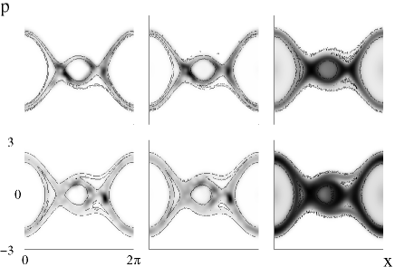
Figure 1: Classical (contour lines) and quantum (gray scale density plot) phase space distributions for $t=50$ (in units of the period of the forcing). In the upper row $F=0.02$ and in the lower one $F=0.05$. We display the cases (from left to right) for $T=0$, $T=0.01$, and $T=0.1$. In all cases $\Gamma=10^{-4}$ and $\hbar=0.041$.

The imbalance between the positive and negative $p$ regions of phase space, which is responsible for the current, is significantly altered by varying the parameter $F$. For $F=0.02$ and $T=0$ (see Fig. 1, upper row, leftmost panel) there is a branch of the chaotic region that develops for $p<0$ and that is not present for $p>0$. For $F=0.05$ and $T=0$ (see Fig. 1, lower row, leftmost panel) the distribution looks more symmetric. This behavior persists at low temperatures ($T=0.01$) as can be seen in the middle column of Fig. 1, for both values of $F$. Finally, for a higher temperature ($T=0.1$) the situation changes, and the distributions look more alike, although some features of the phase space structure seem to survive the thermal fluctuations.

In order to assert if this is the case, we show the current values as a function of time (in units of the period of the forcing) in Figs. 2 (a) (for $F=0.02$) and (b) (for $F=0.05$).

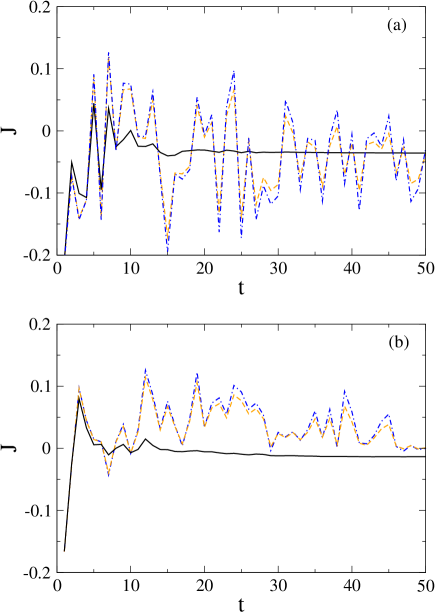
Figure 2: (Color online) Quantum current as a function of time $t$ (in units of the period of the forcing) for the cases shown in Fig. 1. In panel (a) $F=0.02$ and in (b) $F=0.05$. (Blue) dot-dashed lines correspond to $T=0$, (orange) dashed lines to $T=0.01$, and (black) solid lines to $T=0.1$. In all cases $\Gamma=10^{-4}$ and $\hbar=0.041$.

We notice that at $T=0$ (blue dot-dashed lines) there are strong fluctuations that can be associated with the very weak coupling with the environment and the finite $\hbar$ value. At $T=0.01$ (orange dashed lines) the same behavior is present, but at $T=0.1$ (black solid lines) the situation changes and the current stabilizes at very short times ($t\sim 15$), so that a value for the current $J$ can be defined. Moreover, this is valid for both values of $F$. At this point it is worth mentioning that for $F=0.02$ the current is greater than for $F=0.05$, so we can conclude that the quantum distributions preserve the main features of the original structure of phase space at $T=0$. This makes the current generation mechanism robust against environmental perturbations in the weak coupling regime. Moreover, temperature also helps to stabilize the ratchet.

To conclude this subsection, we would like to mention that our choice of parameters is suitable for modeling many isomerization reactions induced by laser fields isovision ; isocontrol ; isomerization . The interactions with the solvent can account for the interaction with a thermal environment of the kind that we have analyzed. In this respect, it is interesting to note that the main features for current generation (isomerization rate in this case) survive a weak coupling with the environment, and that this in turn can be beneficial. This suggests that this mechanism is applicable to actual experimental situations.

III.2 Strong forcing

The same system considered above can behave in a quite different way if the strength of the forcing is increased. In fact, when this happens the regular islands structure present in the previous case is completely lost, and then the current arises as a consequence of the asymmetry of a chaotic attractor. In this case, it is easier to define an asymptotic current given the fact that the attractor is usually formed in a very short time. To illustrate this effect, we present in Fig. 3 the classical and quantum phase space distributions for $F=2.5$, $\Gamma=0.05$, and $\hbar=0.041$ at $t=50$. In it, we show from left to right and top to bottom the cases corresponding to: $T=0$, $T=0.001$, $T=0.01$ and $T=0.1$, respectively.

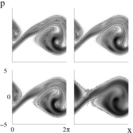
Figure 3: Classical (contour lines) and quantum (gray scale density plot) phase space distributions for $t=50$ (in units of the period of the forcing). From left to right and top to bottom we show the results corresponding to: $T=0$, $T=0.001$, $T=0.01$ and $T=0.1$, respectively. In all cases $F=2.5$, $\Gamma=0.05$ and $\hbar=0.041$.

As in the previous case, the influence of the temperature is noticeable only for its higher value, namely $T=0.1$; while for the rest of the cases the quantum distribution remains almost unchanged. Thermal fluctuations need to be greater than the quantum ones to manifest themselves. This is not the case for the classical attractor, which gradually loses all its finer details. For the set of parameters that we have chosen in this case, the time reversal invariance is only broken by dissipation. Moreover, dissipation is not only responsible for the current generation, but also for the quick stabilization of the current. This can be seen in Fig. 4, where the classical (thin lines) and quantum $J$ as a function of time $t$ are shown.

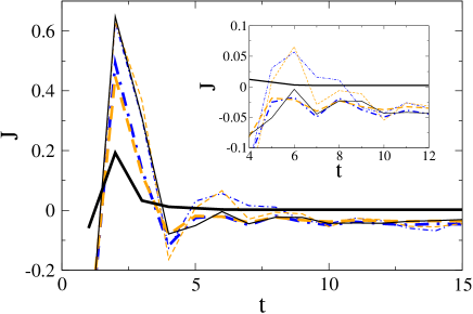
Figure 4: (Color online) Classical (thin lines) and quantum current as a function of time $t$ (in units of the period of the forcing) for some of the cases shown in Fig. 3. (Blue) dot-dashed lines correspond to $T=0$, (orange) dashed lines to $T=0.01$, and (black) solid lines to $T=0.1$. In all cases $F=2.5$, $\Gamma=0.05$ and $\hbar=0.041$. In the inset we show enlarged the stabilization region for the sake of clarity.

As can be seen, for $T=0$ and $T=0.01$ the attractor needs $\sim 10$ periods of the forcing to set in; at this point the current is very well defined, both classical and quantum mechanically. Actually, the correspondence between the quantum and classical results is remarkable. For $T=0.1$ the setting in of the attractor is even faster (just $\sim 6$ periods are needed), but in this case the effect of temperature on the quantum current is rather drastic, i.e. $J$ goes to zero. We have further verified this behavior by using a highly efficient diagonalization method futurework . This allowed us to look into the details of the superoperator spectrum, for which the spectral gap is around $0.4$ (this gap is the distance between the modulus of the leading eigenvalue - equal to one - and the modulus corresponding to the next eigenvalue, in descending order of this quantity). We have also obtained the associated equilibrium eigenvector (corresponding to the eigenvalue one), which resulted indistinguishable from the chaotic attractor found by means of the time evolution.

In order to show the ability of our method to reach the semiclassical limit we consider the classical and quantum chaotic attractors corresponding to $\hbar\simeq 0.0015$ and $T=0$ in Fig. 5. Let us mention here that the study of the evolution of different quantities as a function of time is an interesting sub-product of our approach. Thanks to this, we have found that despite the greater accuracy in the details of the phase space distributions attained in this case, the values of $J$ as a function of $t$ remain essentially the same as for $\hbar=0.041$.

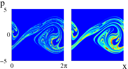
Figure 5: (Color online) Classical (left panel) and quantum (right panel) phase space distributions at time $t=50$ corresponding to $T=0$. In all cases $F=2.5$, $\Gamma=0.05$ and $\hbar\simeq 0.0015$.

IV Conclusions

In this paper, we have studied a ratchet system consisting of a particle moving in a biharmonic potential subjected to a time periodic forcing and in contact with a heat bath at finite temperature. The rich structure of the phase space for different values of the involved parameters has been analyzed both classical and quantum mechanically.

We have found that for weak forcing and very weak coupling with the environment, the mechanism leading to current generation survives. In fact, the quantum distributions keep “memory” of the original structure of the chaotic region at $T=0$. Moreover the effect of the temperature is beneficial, rather than destructive, and the current stabilizes after short times. This makes us suggest a possible experimental verification of these results in chemical isomerization reactions, to which the dynamics we have analyzed can be directly applicable. In the case of the strong forcing regime, the effect of temperature also shorten the times for which the stabilization of the current occurs. But in this case, the current vanishes for higher values of $T$, due to the blurring of the chaotic attractor details (and asymmetry).

Finally, it is worth mentioning the high precision and simplicity of our integration method. By developing a modified split operator scheme, we have been able to reach very low values of $\hbar$. This, combined with a highly efficient diagonalization method will allow us to implement in the near future an alternative approach for studying time dependent dissipative quantum systems futurework .

- (1) R. P. Feynman, Lectures on Physics, Vol. 1, (Addison-Wesley, Reading, MA, 1963).
- (2) P. Reimann, Phys. Rep. 361, 57 (2002).
- (3) S. Flach, O. Yevtushenko, and Y. Zolotaryuk, Phys. Rev. Lett. 84, 2358 (2000); S. Denisov and S. Flach, Phys. Rev. E 64, 056236 (2001); S. Denisov, J. Klafter, M. Urbakh, and S. Flach, Physica D 170, 131 (2002).
- (4) H. Schanz, M.-F. Otto, R. Ketzmerick, and T. Dittrich, Phys. Rev. Lett. 87, 070601 (2001); S. Denisov, J. Klafter, and M. Urbakh, Phys. Rev. E 66, 046203 (2002); H. Schanz, T. Dittrich, and R. Ketzmerick, Phys. Rev. E 71, 026228 (2005).
- (5) P. Reimann, M. Grifoni, and P. Hänggi, Phys. Rev. Lett. 79, 10 (1997); I. Franco and P. Brumer, Phys. Rev. Lett. 97, 040402 (2006).
- (6) L. Ermann, G.G. Carlo, and M. Saraceno, Phys. Rev. E 77, 011126 (2008); L. Ermann, G.G. Carlo, and M. Saraceno, Phys. Rev. E 79, 056201 (2009).
- (7) S. Denisov, L. Morales-Molina, S. Flach, and P. Hänggi, Phys. Rev. A 75, 063424 (2007).
- (8) F. Jülicher, A. Ajdari and J. Prost, Rev. Mod. Phys. 69, 1269 (1997).
- (9) R. D. Astumian, Science 276, 917 (1997).
- (10) C. Mennerat-Robilliard, D. Lucas, S. Guibal, J. Tabosa, C. Jurczak, J.-Y. Courtois, and G. Grynberg, Phys. Rev. Lett. 82, 851 (1999); P. H. Jones, M. Goonasekera, D.R. Meacher, T. Jonckheere, and T.S. Monteiro, Phys. Rev. Lett. 98, 073002 (2007); T. Salger, S. Kling, T. Hecking, C. Geckeler, L. Morales-Molina, and M. Weitz, Science 326, 1241 (2009).
- (11) F. L. Moore, J. C. Robinson, C. F. Bharucha, B. Sundaram, and M. G. Raizen, Phys. Rev. Lett. 75, 4598 (1995); T. S. Monteiro, P. A. Dando, N. A. C. Hutchings, and M. R. Isherwood, Phys. Rev. Lett. 89, 194102 (2002); G. G. Carlo, G. Benenti, G. Casati, S. Wimberger, O. Morsch, R. Mannella, and E. Arimondo, Phys. Rev. A 74, 033617 (2006).
- (12) M. Sadgrove, M. Horikoshi, T. Sekimura, and K. Nakagawa, Phys. Rev. Lett. 99, 043002 (2007); I. Dana, V. Ramareddy, I. Talukdar, and G.S. Summy, Phys. Rev. Lett. 100, 024103 (2008).
- (13) E. Lundh and M. Wallin, Phys. Rev. Lett. 94, 110603 (2005); E. Lundh, Phys. Rev. E 74 016212 (2006); D. Poletti, G. G. Carlo, and B. Li, Phys. Rev. E 75, 011102 (2007).
- (14) A. Kenfack, J. Gong, and A.K. Pattanayak, Phys. Rev. Lett. 100, 044104 (2008); J. Wang and J. Gong, Phys. Rev. E 78, 036219 (2008).
- (15) M. Sadgrove, M. Horikoshi, T. Sekimura, and K. Nakagawa, Eur. Phys. J. D 45, 229 (2007).
- (16) R. W. Schoenlein, L. A. Peteanu, R. A. Mathies, and C. V. Schank, Science 254, 412 (1991); J. E. Kim, J. Tauber, and R. A. Mathies, Biochemistry 40, 13774 (2001); D. Polli, P. Altoe, O. Weingart, K. M. Spillane, C. Manzoni, D. Brida1, G. Tomasello, G. Orlandi, P. Kukura, R. A. Mathies, M. Garavelli, and G. Cerullo, Nature 467, 440 (2010).
- (17) F. Garczarek and K. Gerwert, Nature 439, 109 (2006).
- (18) G. Voght, G. Krampert, P. Niklaus, P. Nuerberger, and G. Gerber, Phys. Rev. Lett. 94, 068305 (2005); M. Abe, Y. Ohtsuki, Y. Fujimura, and W. Domcke, J. Chem. Phys. 123, 144508 (2005); V.I. Prokhorenk, A.M. Nagy, S.A. Waschuk, L.S. Brown, R.R. Birge, R.J. Dwayne Miller, Science 313, 125 (2006).
- (19) G. E. Murgida, D. A. Wisniacki, P. I. Tamborenea, and F. Borondo, Chem. Phys. Lett. 496, 356 (2010).
- (20) J. Gong, A. Ma, and S. A. Rice, J. Chem. Phys. 122, 144311 (2005); ibid. 122, 204505 (2005); Maxim A., T.-S. Ho, H. Rabitz, Chem. Phys. 328, 147 (2006); P.L. García-Müller, F. Borondo, R. Hernandez, and R. M. Benito, Phys. Rev. Lett. 101, 178302 (2008).
- (21) G. G. Carlo, G. Benenti, G. Casati, and D.L. Shepelyansky, Phys. Rev. Lett. 94, 164101 (2005).
- (22) S. Denisov, S. Kohler, and P. Hanggi, Europhys. Lett. 85, 40003 (2009).
- (23) P.K. Ghosh and D.S. Ray, Phys. Rev. E 73, 036103 (2006); G.G. Carlo and M.E. Spina, Phys. Rev. E 79, 026212 (2009).
- (24) S.A. Maier and J. Ankerhold, arXiv:1006.0433.
- (25) I. Pavlyukevich, B. Dybiec, A. V. Chechkin, and I. M. Sokolov, arXiv:1008.4246.
- (26) A.B. Kolton and F. Renzoni, Phys. Rev. A 81, 013416 (2010).
- (27) Juha Javanainen and Janne Ruostekoski, J. Phys. A: Math. Gen. 39, L179 (2006).
- (28) C.W. Gardiner and P. Zoller, Quantum Noise (Springer-Verlag, Berlin, 1991).
- (29) G.G. Carlo, G. Benenti, G. Casati, and C. Mejía-Monasterio, Phys. Rev. A 69, 062317 (2004).
- (30) L. Ermann, G.G. Carlo, F. Borondo, and R.M. Benito, in preparation.