Localized mode interactions in 0-$\pi$ Josephson junctions

Abstract

A long Josephson junction containing regions with a phase shift of $\pi$ is considered. By exploiting the defect modes due to the discontinuities present in the system, it is shown that Josephson junctions with phase-shift can be an ideal setting for studying localized mode interactions. A phase-shift configuration acting as a double-well potential is considered and shown to admit mode tunnelings between the wells. When the phase-shift configuration is periodic, it is shown that localized excitations forming bright and dark solitons can be created. Multi-mode approximations are derived confirming the numerical results.

Introduction. A Josephson junction is a system consisting of two layers of superconductors separated by a nonsuperconducting barrier. Electrons forming so-called Cooper pairs can tunnel across the resistive barrier even when there is no applied voltage difference. Theoretically predicted by Josephsonjose62 and first observed experimentally in Ref. ande63, , the only requirement for the occurrence of Josephson tunneling is a weak coupling of the wave functions of the two superconductors. The supercurrent ($I_{s}$) is proportional to the sine of the electron phase-difference across the insulator ($u$), i.e. $I_{s}\sim\sin{u}$.

Bulaevskii et al.bula77 ; bula78 proposed that a shift of $\pi$ can be introduced in the phase difference $u$ of a Josephson junction by installing magnetic impurities, which has been confirmed recentlyvavr06 . Present technological advances can also impose a $\pi$-phase-shift in a long Josephson junction using various means, including multilayer junctions with controlled thicknesses over the insulating barrierryaz01 ; base99 , pairs of current injectors gold04 , and junctions with unconventional order parameter symmetrytsue00 ; hilg03 ; guma07 .

New phenomena may occur when a junction with phase-shifts is connected to a normal junction, i.e. 0-$\pi$ Josephson junctions. These include the presence of a half magnetic flux quantum induced by spontaneously created supercurrent circulating in a loop. Such unique characteristics offer promising future device applications, such as novel circuits for information storage and processing in both classical and quantum limitsgold05 and artificial crystals for simulating and studying energy levels and band structures in large systems of spinssusa05 (see also Ref. hilg08, and references therein). Here, we demonstrate that Josephson junctions with phase-shifts is an ideal setting for showcasing many interesting features of localized mode interactions. Arguably the dynamics of the superconductor phase-difference can be seen to be analogues to that of atomic wave functions of Bose-Einstein condensates (BEC)bose24 ; eins25 ; ande95 ; davi95 ; brad97 in an external potential. In particular, we consider Josephson junctions with phase-shift configurations acting as a double well and a periodic potential.

The interesting phenomenon of mode tunneling in BECs in a double well potential was predicted by Smerzi et al. smer97 ; giov00 , followed by experimental observationsalbi05 ; lebl10 . Here, we will show that defect modes due to the presence of phase-discontinuities in $0$-$\pi$ Josephson junctions can be exploited to observe a similar mode tunneling, which can also be viewed as Rabi oscillations of two interacting modes.ostr00 Periodic defects exhibiting mode self-trapping analogues to BECs in optical latticesmors06 will also be discussed.

Double-well potential. A 0-$\pi$ Josephson junction with the superconductor phase difference $u$ at position $x$ and time $t$ is described by the sine-Gordon equation

$$u_{tt}-u_{xx}=-\theta(x)\sin{u},$$ (1)

where $x$ and $t$ have been normalized to the Josephson penetration depth $\lambda_{J}$ and the inverse plasma frequency $\omega_{p}^{-1}$, respectively. The function $\theta(x)$ is piecewise constant representing the presence of $\pi$ junctions. A double well potential with two $\pi$-junctions of length $a$ separated by a $0$-junction with length $2L$ is described by

$$\theta(x)=\left\{\begin{array}[]{rl}-1,&\quad L<|x|<L+a,\\ 1,&\quad\rm{elsewhere}.\end{array}\right.$$ (2)

At the points of discontinuities, the boundary conditions are

$$\begin{array}[]{rcl}\displaystyle\lim_{x\to\pm\{L,L+a\}^{+}}u(x,t)&=&\displaystyle\lim_{x\to\pm\{L,L+a\}^{-}}u(x,t);\\ \displaystyle\lim_{x\to\pm\{L,L+a\}^{+}}u_{x}(x,t)&=&\displaystyle\lim_{x\to\pm\{L,L+a\}^{-}}u_{x}(x,t).\end{array}$$ (3)

If $\phi$ solves (1), the linear stability of the solution can be analyzed by substituting the spectral ansatz $u=\phi+v(x)e^{\lambda t}$ and linearizing about $||v||_{\infty}$ small to yield the eigenvalue problem $v_{xx}-\lambda^{2}v=\theta\cos(\phi)v.$

Equation (1) has two constant solutions (mod $2\pi$), $u\equiv 0$ and $u\equiv\pi$. The solution $u\equiv\pi$ has unstable continuous spectrum and hence is always unstable.susa03 The solution $u=0$ has stable continuous spectrum $\lambda^{2}<-1$ and the discrete spectrum (eigenvalues) can be calculated analytically.susa03 Indeed, the largest two eigenvalues $\Lambda_{\pm}$ of $u=0$ solve the equation

$$\frac{\sqrt{1-\Lambda_{\pm}^{2}}}{\tan\left(\sqrt{1-\Lambda_{\pm}^{2}}a\right)}+\Lambda_{\pm}\mp e^{-2\sqrt{1+\Lambda_{\pm}}L}=0.$$ (4)

The corresponding eigenmodes $\Phi_{\pm}(x)$ of $\Lambda_{\pm}$ aresusa03

$$\Phi_{\pm}=\left\{\begin{array}[]{ll}e^{-\sqrt{1+\Lambda_{\pm}}(x-L-a)},&\,x>L+a;\\ \cos(\sqrt{1-\Lambda_{\pm}}(x-L-a))\\ {}+C\,\sin(\sqrt{1-\Lambda_{\pm}}(x-L-a)),&\,L<x<L+a;\\ K_{+}\,\cosh(\sqrt{1+\Lambda_{\pm}}x)\\ {}+K_{-}\,\sinh(\sqrt{1+\Lambda_{\pm}}x),&\,0<x<L,\end{array}\right.$$ (5)

where $C=-\sqrt{\frac{1+\Lambda_{\pm}}{1-\Lambda_{\pm}}}$ and $K_{\pm}=\frac{2e^{-\sqrt{1+\Lambda_{\pm}}L}\sin(\sqrt{1-\Lambda_{\pm}}a)}{\sqrt{1-\Lambda_{\pm}^{2}}}$. As the linearisation operator is a Sturm-Liouville operator and even in $x$, the eigenmodes are simple and the eigenfunction $\Phi_{+}$ is an even function and $\Phi_{-}$ is odd. The two eigenvalues $\Lambda_{\pm}$ are depicted as a function of $a$ for fixed $L=2$ (to the left of the vertical dashed line).

It is clear that $u=0$ has a stability window. The change of stability occurs at a critical distance $a_{c}$ when the critical eigenvalue crosses the horizontal axis $\Lambda=0$. Using the expression in (4), it follows that the critical length $a_{c}(L)$ is $a_{c}=\arctan(e^{2L})$.

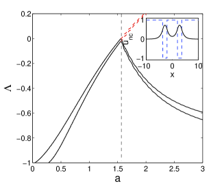
Figure 1: The eigenvalues of the ground state as a function of $a$ for $L=2$. The dashed vertical line indicates the bifurcation point of the non uniform ground state, where on the left and on the right of the vertical line $u=0$ is stable and unstable, respectively. The dashed lines show the eigenvalues of the uniform solution in its instability region. The inset presents a ground state when $L=2$ and $a=1.65$.

In the instability region, a non uniform time-independent sign-definite ground state $\pm u_{nc}(x)$ bifurcates. Its expression can be written in terms of Jacobian elliptic functions susa03 ; zenc04 as

$$u_{nc}=\left\{\begin{array}[]{rl}4\arctan(e^{-x+x_{0}}),&\,x>L+a;\\ 2\arcsin(m_{1}\mathop{\rm sn}(x-x_{1},m_{1})),&\,L<x<L+a;\\ \pi+2\arcsin(m_{2}\mathop{\rm sn}(x-x_{2},m_{2})),&\,0<x<L.\end{array}\right.$$ (6)

The parameters $m_{1}$ and $m_{2}$ are linked to the lengths $a$ and $L$ by

$$\begin{array}[]{rcl}a&=&2K(m_{1})-\mathop{\rm am}^{-1}(\pi/4,m_{1})\\[2.84526pt] &&-\mathop{\rm am}^{-1}(\arcsin(\sqrt{2(1+m_{1}^{2}-m_{2}^{2})}/2m_{1}),m_{1})\\[2.84526pt] L&=&K(m_{2})-\mathop{\rm am}^{-1}(\arcsin(\sqrt{2(1+m_{2}^{2}-m_{1}^{2})}/2m_{2}),m_{2})\end{array}$$

The translations $x_{i}$ are determined by the boundary conditions (3). The non-uniform ground state and its eigenvalues are presented in Fig. 1 (to the right of the vertical dashed line).

Mode tunneling. In the following, let us first consider $L=2a=2$. For those parameter values, $u=0$ is a stable ground state. The numerically obtained time dynamics of an initially localized excitation in the left well is presented in the top panels of Fig. 2, clearly showing mode tunneling. Compare it with the time dynamics of BECs reported in Refs. smer97, ; giov00, ; albi05, ; lebl10, .

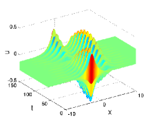
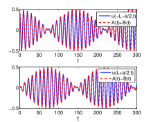
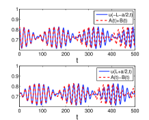
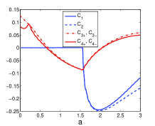
Figure 2: (Color online) Panel (a) shows the time dynamics of an initially localized excitation in the left well with $L=2$ and $a=1$. In panel (b), the oscillation amplitudes of the dynamics presented in panel (a) are plotted against time. Panel (c) depicts the oscillation amplitude on top of a nonzero background with a small initial amplitude for a double well with $L=2$ and $a=1.65$. Coupling coefficients appearing in (10) as functions of $a$ for $L=2$ are shown in panel (d). In calculating the coefficients, the eigenfunctions have been normalized to $||\Phi_{\pm}||_{\infty}=1.$ Approximations obtained from the two-mode equation (10) are shown as red dashed curves.

Next, we consider a parameter combination of $L=2$ and $a=1.65$, i.e. $u=0$ is unstable. In the instability region of the constant solution, excitations will oscillate on a non-zero background $u_{nc}$ (6). The oscillation amplitude in both wells as a function of time is presented in panel (c) of Fig. 2. When the initial oscillation amplitude is large enough, we interestingly obtain chaotic oscillations (not shown here).

Two-mode approximations. We will explain the observed mode tunneling using a two-mode approximation. Looking for the solution of the time-dependent equation (1) of the form

$$u(x,t)=u_{gs}+A(t)\Phi_{+}+B(t)\Phi_{-},$$ (7)

where $u_{gs}$ is the ground state of the system, i.e. $u_{gs}=0$ and $u_{gs}=u_{nc}$ when $a$ is respectively on the left and right of the vertical line in Fig. 1, substituting the ansatz (7) into (1), and projecting the equation onto $\Phi_{\pm}$ will yield up to $\mathcal{O}(A^{n}B^{4-n}),\,n=0,\dots,4$

$$\displaystyle\begin{array}[]{lll}\ddot{A}&=&\Lambda_{+}A+\left(C_{1}A^{2}+C_{2}B^{2}\right)+\left(C_{3+}A^{3}+C_{4+}AB^{2}\right);\\ \ddot{B}&=&\Lambda_{-}B+\left(C_{3-}B^{3}+C_{4-}A^{2}B\right);\end{array}$$ (10)

with

$$C_{1}=\frac{K_{+}}{2}\,\int_{-\infty}^{\infty}\theta\sin(u_{gs})\Phi_{+}^{3}\,dx,$$ (11)

$$C_{2}=\frac{K_{+}}{2}\,\int_{-\infty}^{\infty}\theta\sin(u_{gs})\Phi_{+}\Phi_{-}^{2}\,dx,$$ (12)

$$C_{3\pm}=\frac{K_{\pm}}{6}\,\int_{-\infty}^{\infty}\theta\cos(u_{gs})\Phi_{\pm}^{4}\,dx,$$ (13)

$$C_{4\pm}=\frac{K_{\pm}}{6}\,\int_{-\infty}^{\infty}\theta\cos(u_{gs})\Phi_{+}^{2}\Phi_{-}^{2}\,dx,$$ (14)

and $K_{\pm}=\left(\int_{-\infty}^{\infty}\Phi_{\pm}^{2}dx\right)^{-1}$. The constants $C_{j}$ are plotted against $a$ in panel (d) of Fig. 2. The internal oscillation amplitude $u\left(\pm(L+a/2),t\right)$ is respectively approximated by $u_{gs}+(A(t)\pm B(t))/2$.

For the uniform ground state ($u_{gs}=0$), we have solved (10) numerically and compared it with the oscillation amplitude of the original equation in panel (b) of Fig. 2. One can observe that quantitative agreements are obtained. An agreement is also obtained for mode tunneling on a non-uniform background, as shown in panel (c) of Fig. 2, provided that the tunneling mode amplitude is small enough.

When $A(0)$ and $B(0)$ are large, it is interesting to note that even though our two-mode approximation does not quantitatively capture the dynamics of the chaotic tunnelings it captures the qualitative transition to chaotic behavior.

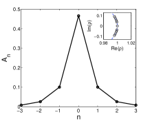
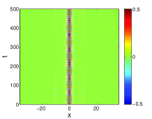
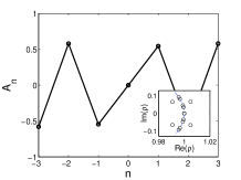
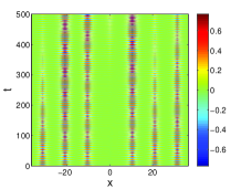
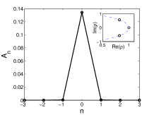
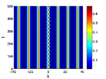
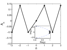
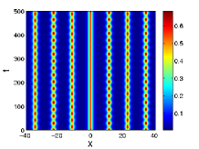
Figure 3: (Color online) The left panels show the profile of numerically exact bright and dark lattice solitons obtained from the lattice equation (18). The insets depict the Floquet multipliers of the solution. The right panels present the corresponding time dynamics of (1) using the initial condition (17) with $A_{n}(0)$ shown in the adjacent left panel. All panels have $L=10$, the upper two have $a=0.5$, the lower $a=1.6$.

Periodic defects. One can also include more phase shifts and derive a multi-mode approximation. Below we consider the case of periodic shifts alternating $\pi$-junctions of length $a$ with $0$-junctions of length $L$, i.e.,

$$\theta=\left\{\begin{array}[]{ll}-1,&x\in k(L+a)+(-\frac{a}{2},\frac{a}{2}),k\in\mathbb{Z}\\ 1,&\rm{elsewhere}.\end{array}\right.$$ (15)

It is known that in the limit $L\to\infty$ (i.e., one well), $u=0$ is stable for $a<\pi/4$ and unstable otherwise susa03 . The eigenfunction corresponding to the critical eigenvalue $\Lambda_{0}$ of the ground state $u_{gs}$ in the limit $L\to\infty$ will be denoted by $\Phi_{0}(x)$. For $a<\pi/4$ and $u_{gs}=0$,

$$\Phi_{0}(x)=\left\{\begin{array}[]{ll}\cos(\sqrt{1-\Lambda_{0}}a)e^{-\sqrt{1+\Lambda_{0}}\left(|x|-a/2\right)},&|x|>a/2,\\ \cos(\sqrt{1-\Lambda_{0}}x),\,|x|<a/2.\end{array}\right.$$ (16)

When $L\gg 1$, a tight-binding approximation can be used to describe the interaction of the defect modes in the system with periodic defects. We write

$$u(x,t)=u_{gs}+\sum_{n=-\infty}^{\infty}A_{n}(t)\Phi_{n}(x),$$ (17)

where $\Phi_{n}(x)=\Phi_{0}\left(x-n(a+L)\right)$. Performing the same procedure as before, one will obtain the lattice equation

$$\ddot{A}_{n}=\Lambda_{0}A_{n}+K_{2}A_{n}^{2}+K_{3}A_{n}^{3}$$

$$+\!\sum_{j=\pm 1}\!\!\!C_{j}[(K_{1,j}-\Lambda_{0})A_{n+j}-K_{2}A_{n+j}^{2}-K_{3}A_{n+j}^{3}],$$ (18)

where

$$C_{\pm 1} = K^{(0)}\int_{-\infty}^{\infty}\ \Phi_{0}(x)\Phi_{\pm 1}(x)\,dx,$$

$$K_{1,\pm 1} = C_{\pm}^{-1}K^{(0)}\int_{-\infty}^{\infty}\Phi_{0}(x)\left(\partial_{x}^{2}-\theta\cos{u_{gs}}\right)\Phi_{\pm 1}(x)\,dx,$$

$$K_{2} = K^{(0)}\int_{-\infty}^{\infty}\frac{1}{2}\sin(u_{gs})\Phi_{0}^{3}(x)\,dx,$$

$$K_{3} = K^{(0)}\int_{-\infty}^{\infty}\frac{1}{6}\cos(u_{gs})\Phi_{0}^{4}(x)\,dx,$$

and $K^{(0)}=\left(\int_{-\infty}^{\infty}\Phi_{0}^{2}\,dx\right)^{-1}.$ Neglecting the nonlinear couplings to the neighboring sites ($CK_{2},\,CK_{3}$), the discrete equation above becomes the lattice equation considered by Kivsharkivs93 , admitting many types of localized excitations. In the following, we consider the special type, namely unstaggered bright and staggered dark lattice solitons. In particular, we will show that the lattice equation (18) can predict the stability of the solitons in the original equation (1), provided that $L$ is large enough. In doing so, we first solve Eq. (18) numerically for localized modes using a shooting method and correspondingly study their stability (see, e.g., the review Ref. flac04, ) and then use the ansatz (17) at $t=0$ as an initial condition for the governing equation (1). In the following, periodic boundary conditions are used, which are relevant experimentally.gurl10 Examples are shown in Fig. 3. Presented in the left and right panels are numerically exact solutions obtained from the lattice equation (18) and their corresponding time evolution in the original equation (1). The insets on the left panels depict the corresponding Floquet multipliers, where the instability is indicated by the presence of eigenvalues lying outside the unit circle (dash-dotted line).

First, we consider the parameter values $L=10$ and $a=0.5$, representing the case of stable constant solution $u=0$. Shown in the first and the second row are numerically exact bright and dark solitons with the oscillation period $P=7.08$ ($\Lambda_{0}\approx-0.8$) and their dynamics. According to the lattice equation (18), the bright soliton is stable and the dark one unstable. One can note from the right panels that the prediction provided by the lattice is in agreement with the dynamics in the original system. The instability of the dark soliton manifests in the form of the destruction of the configuration.

Next, we consider the parameter values $L=10$ and $a=1.6$, which represent the case of nonuniform ground state. The localized mode will then oscillate on a nonzero background. Shown in the third and fourth row are numerically exact bright and dark lattice solitons with the oscillation period $P=30$ ($\Lambda_{0}\approx-0.0527$).

According to the lattice equation (18), the bright soliton has the same stability as the case on stable uniform ground state, which is confirmed by the time dynamics of the original equation. The stability of the soliton for the chosen parameter values is not surprising as the sites are rather uncoupled.

As for the dark soliton, it is interesting to note that in the present case it is stable, which is also confirmed by the dynamics of the full equation. This implies that a nonzero background may act as a stabilizer. Moreover, it is also important to note that the modes in different lattices have different oscillation frequencies. The multi-frequency breathers discussed in Ref. kouk02, ; kouk04, may therefore be potentially observed in experiments.

Conclusions. We have considered Josephson junctions with phase-shifts of $\pi$. By exploiting the defect modes present due to the phase-discontinuities, the system has been shown to be an ideal setting for studying mode interactions. In particular, we have shown that mode tunneling in a double-well potential can be implemented in the system and presented the existence and stability of bright and dark solitons in a periodic potential. We have shown that the analysis proved by a multi-mode approximation gives a quantitative agreement with dynamics of the original system.

References

- (1) B.D. Josephson, Phys. Lett. 1, 251 (1962).
- (2) P.W. Anderson and J.M. Rowell, Phys. Rev. Lett. 10, 230 (1963).
- (3) L.N. Bulaevskii, V.V. Kuzii, and A.A. Sobyanin, Pis’ma Zh. Eksp. Teor. fiz. 25, 314 (1977) [JETP Lett. 25, 290 (1977)].
- (4) L.N. Bulaevskii, V.V. Kuzii, and A.A. Sobyanin, Solid State Comm. 25, 1053 (1978).
- (5) O. Vávra et al., Phys. Rev. B 74, 020502 (2006).
- (6) V.V. Ryazanov et al., Phys. Rev Lett. 86, 2427 (2001).
- (7) J.J.A. Baselmans et al., Nature 397, 43 (1999).
- (8) E. Goldobin et al., Phys. Rev. Lett. 92, 057005 (2004).
- (9) C.C. Tsuei and J.R. Kirtley, Rev. Mod. Phys. 72, 969 (2000).
- (10) H. Hilgenkamp et al., Nature 422, 50 (2003).
- (11) A. Gumann, C. Iniotakis, and N. Schopohl, Appl. Phys. Lett. 91, 192502 (2007).
- (12) E. Goldobin et al., Phys. Rev. B 72, 054527 (2005).
- (13) H. Susanto et al., Phys. Rev. B 71, 174510 (2005).
- (14) H. Hilgenkamp, Supercond. Sci. Technol. 21, 034011 (2008).
- (15) S.N. Bose, Zeit. Phys. 26, 178 (1924).
- (16) A. Einstein, Sber. Preuss. Akad. Wiss. 22, 261 267 (1924); ibid. 1, 3 14 (1925).
- (17) M.H. Anderson et al., Science 269, 198 201 (1995).
- (18) K.B. Davis et al., Phys. Rev. Lett. 75, 3969 3973 (1995).
- (19) C.C. Bradley et al., Phys. Rev. Lett. 75, 1687 1690 (1995).
- (20) A. Smerzi et al., Phys. Rev. Lett. 79, 4950 (1997).
- (21) S. Giovanazzi et al., Phys. Rev. Lett. 84, 4521 (2000).
- (22) M. Albiez et al., Phys. Rev. Lett. 95, 010402 (2005).
- (23) L.J. LeBlanc et al., arXiv:1006.3550.
- (24) E. A. Ostrovskaya et al., Phys. Rev. A 61, 031601-4 (2000).
- (25) O. Morsch and M. Oberthaler, Rev. Mod. Phys. 78, 179 (2006).
- (26) H. Susanto et al., Phys. Rev. B 68, 104501 (2003).
- (27) A. Zenchuk and E. Goldobin, Phys. Rev. B 69, 024515 (2004).
- (28) Yu.S. Kivshar, Phys. Lett. A 173, 172-178 (1993).
- (29) S. Flach in: Energy Localization and Transfer, Eds. T. Dauxois et al, World Scientific (2004), pp. 1-71.
- (30) C. Gürlich et al., Phys. Rev. B 81, 094502 (2010).
- (31) V. Koukouloyannis, Phys. Rev. E 69, 046613 (2004).
- (32) V. Koukouloyannis and S. Ichtiaroglou, Phys. Rev. E 66, 066602 (2002).