Variational approximations to homoclinic snaking
Abstract
We investigate the snaking of localised patterns, seen in numerous physical applications, using a variational approximation. This method naturally introduces the exponentially small terms responsible for the snaking structure, that are not accessible via standard multiple-scales asymptotic techniques. We obtain the symmetric snaking solutions and the asymmetric ‘ladder’ states, and also predict the stability of the localised states. The resulting approximate formulas for the width of the snaking region show good agreement with numerical results.
There has been much recent interest in the phenomenon of spatially localised patterns, budd05 ; burk07 ; chap09 ; kozy06 , extending our understanding of earlier work on this topic pome86 ; bens88 . As discussed in the review article by Dawes dawe10 , this work is motivated by wide-ranging applications in many different areas of physics, including buckling of struts and cylinders cham98 ; hunt00 ; wade99 , nonlinear optics chap09 , convection patterns bens88 ; nepo94 , gas discharge systems and granular media. Most theoretical work concentrates on the Swift-Hohenberg equation, which is the simplest model equation that illustrates the effect bens88 ; dawe10 ; kozy06 .
These localised patterns arise as a result of bistability between a uniform state and regular patterned state. A front linking these two states might be expected to move in one direction or the other, except at a specific parameter value, referred to as the Maxwell point. However, due to a pinning effect first described qualitatively by Pomeau pome86 , the front can lock to the pattern, resulting in a finite range of parameter values around the Maxwell point where a stationary front can exist. Combining two such fronts leads to a pinned localised state. The pinning range is seen in numerical simulations saka96 ; wood99 ; burk06 ; burk07 ; burk07_2 and leads to a ‘snaking’ bifurcation diagram in which the control parameter oscillates about the Maxwell point as the size of the localised pattern increases.
The localised states can also been seen from the viewpoint of spatial dynamics as a homoclinic connection from the uniform state to itself, leading to a geometrical argument for the existence of such states over a finite range of parameter values coul00 ; cham98 ; hunt00 .
It has been appreciated for some time pome86 that the pinning effect cannot be described by conventional multiple-scales asymptotics, since this method treats the scale of the pattern and the scale of its envelope as independent variables, leading to an arbitrary phase in the envelope function. Hence, the pinning range is ‘beyond all orders’, or is exponentially small in the small parameter corresponding to the pattern amplitude bens88 . A very thorough analysis of the exponential asymptotics of this problem has recently been carried out by Kozyreff and Chapman kozy06 ; chap09 , extending earlier work yang97 ; wade99 . The calculation of the pinning range is extremely complicated and unfortunately requires two fitting parameters.
Many previous authors have noted the variational property of the Swift-Hohenberg equation budd05 ; nepo94 ; burk07 , but have not made use of this in regard to the snaking diagram. Wadee and Bassom wade00 did use the variational method, but not in the snaking regime. In this Letter we exploit the variational structure of the Swift-Hohenberg equation in order to approximate the pinning range. An ansatz based on the weakly nonlinear solution is substituted into the Lagrangian of the system, and then this is minimised over the unknown parameters. This approach has a number of advantages: the calculations are much less cumbersome than those involved in the full exponential asymptotics analysis; exponentially small terms appear naturally through the evaluation of the Lagrangian integral; there are no unknown constants that have to be determined by fitting with numerical results; and the corresponding effective Lagrangian can predict the stability of the states. Although the method is widely applicable, for illustrative purposes we consider the cubic-quintic Swift-Hohenberg equation burk07 ; dawe10 ; nepo94 . The results are then compared with numerics.
The governing equation is given by
| (1) |
where is the control parameter and and are the coefficients of the cubic and quintic term, respectively. The uniform state is unstable for . The interesting case leading to snaking bifurcations is , , in which case localised solutions can exist for . It is possible to rescale to set but we will keep as a parameter for consistency with budd05 ; burk07 .
The stationary solutions of (1) can be derived from a Lagrangian
| (2) |
which is finite since we are concerned with localised solutions. Furthermore,
| (3) |
so stable solutions correspond to minima of and can be interpreted as the total ‘energy’ of a solution. The -norm of the solution is defined as .
Motivated by weakly nonlinear analysis bens88 ; burk07 ; wade99 we study two forms of localised pattern. For small , we write the localised solution of (1) as
| (4) |
Using, e.g., complex variable techniques, substituting the approximation (4) into the Lagrangian (2) yields the effective Lagrangian
| (5) | |||||
where
Note that the terms involving the phase shift in (5) have an exponential factor. Therefore, it is expected that the splitting of localized solutions with different phase in the limit , i.e. and , is exponentially small, as suggested in wade99 ; kozy06 ; chap09 . For the ansatz (4)
which is the square of the norm.
Applying the Euler-Lagrange formulation to the effective Lagrangian
| (6) |
gives us a system of nonlinear equations for , and that make (4) an approximate solution of (1). Neglecting the exponentially small terms, (6) can be solved perturbatively to yield (up to )
| (7) | |||||
| (8) | |||||
| (9) |
Note that the leading order expansions above are the same as those obtained using multiple scale expansions burk07 . The phase-shift at this order is arbitrary, which also agrees with the multiple scales result. However, taking into account the equation , in which all the terms are exponentially small, is a multiple of , i.e. there are two different types of solution, odd or even in . This same conclusion was reported in wade99 after a lengthy ‘beyond all orders’ calculation.
It is expected that the ansatz (4) only resembles exact solutions of the Swift-Hohenberg equation when is order 1 and is small. Computations of snaking are generally carried out with neither nor being small budd05 ; burk07 ; saka96 . For localised states in the snaking regime, the envelope solution has a plateau, which becomes longer as the norm increases. As the Maxwell point is the center of the snaking, it is reasonable to construct homoclinic snaking solutions using a special solution at that point, i.e. a front solution.
We approximate the solution in the snaking region by
| (10) |
When the modulus sign in the denominator is absent, the solution (10) forms a front solution at the Maxwell point obtained using a multiple-scales expansion method for small and small bens88 ; nepo94 ; budd05 . Due to the modulus sign, (10) patches two fronts of opposite polarity, leading to a localised state of length . Even though the derivative of this solution is not continuous at , it is smooth enough when , which we assume to be the case (i.e. the fronts are well separated). To simplify the algebra we set .
Substituting the ansatz (10) into the Lagrangian (2), the effective Lagrangian can be obtained as
| (11) | |||||
To illustrate some of the steps in the calculation, consider the term . This can be written as
after using the double-angle formula and the fact that the envelope function is even. The first term in the integral can be evaluated directly and gives the answer . The second term can be found by writing Re and using contour integration. The integrand has simple poles at , but the first of these dominates, giving an exponentially small contribution of order . Evaluating the residue in the standard way gives the leading-order result
| (12) |
The other terms in can be evaluated in a similar way, using poles of order up to three. The formula (12) gives the square of the norm , indicating that in the snaking region, solutions with a larger norm correspond to longer plateaus.
Consider first the terms in (11) that are not exponentially small, and assume that so that the term may be neglected. Making these terms stationary with respect to , and and solving them for , and gives , , and , with
| (13) |
which are the parameter values of the front at the Maxwell point, in exact agreement with the multiple-scales asymptotic method bens88 ; nepo94 ; budd05 . Note that depends linearly on , but this dependence vanishes at the Maxwell point. This is to be expected since the Maxwell point is determined by the condition that the patterned state has the same energy as the zero state.
Near the Maxwell point we set
After making the above simplifications,
| (14) | |||||
In this form, the Lagrangian can be interpreted more easily. The first two terms are constant and independent of . These arise from the two front regions at the ends of the localised states. The first of these terms dominates for small , being of order . Since this term is positive, localised states have a greater energy than the periodic state or the zero state, so energy considerations suggest that the periodic state or the zero state are ‘preferred’ over localised states. Similarly, multi-pulse localised solutions will have a larger value of , in proportion to the number of pulses.
The third term in (14), proportional to , indicates a preference for increasing values of if , so that the patterned region grows in this case and shrinks if .
Finally we have the exponentially small terms responsible for the snaking. The first of these, proportional to , is larger than the second, for small .
The two remaining undetermined parameters in the ansatz (10) are and . The variation of the effective Lagrangian with respect to and can be readily calculated from (14). From , there are two different possibilities. The first is that , so as in the previous case, is a multiple of . Solving the equation for at leading order in then gives
| (15) |
the plus and minus signs corresponding to the odd and even states respectively. This in turn gives the maximum value of as
| (16) |
The width of the snaking region is therefore approximately given by .
The Lagrangian is then an oscillating function of , intertwining between the Lagrangian with and . There is a periodic sequence of alternating stable and unstable equilibria, corresponding to minima and maxima of the Lagrangian respectively. As is increased, all the equilibria disappear in saddle-node bifurcations at . Near these bifurcations, the stable state is the one of the pair with the lower value of .
The second possibility arising from is that (considering only the larger of the two exponentially small terms in (14)). These types of solutions correspond to the ‘bridge’ wade02 or ‘ladder’ burk07 states that link the snaking branches, and only exist for values of that are multiples of . For these solutions, determines the value of the phase by
| (17) |
Considering as a function of the two variables and , it is easy to see that the snaking solutions are either maxima or minima, while the ladder states are always saddle points. Therefore, the snaking solutions are either stable, or unstable with two positive eigenvalues, and the ladder states are always unstable with one positive eigenvalue. These results are in agreement with numerical simulations (see burk07 ).
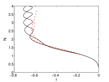
We have found steady localized states of (1) numerically, using a pseudo-arclength continuation method with periodic boundary conditions, implemented with a Fourier spectral discretisation. A summary of the results is shown in Fig. 1.
The top panel shows the bifurcation diagram showing two branches of localized solutions for and . In the same panel, shown in dashed lines are our analytical results (6), showing that the variational calculation approximates the numerics better for relatively small .
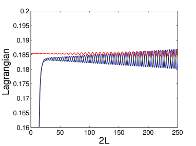
In the middle panel, we plot the Lagrangian (2) for as a function of the length of the solution’s plateau , which is calculated numerically as where and the integration is a definite integration over the computational domain. Plotted in the same panel is our effective Lagrangian (11). There is good agreement for the average numerical value of the Lagrangian and the qualitative nature of the oscillations, but the variational approximation underestimates the amplitude of the oscillations. The amplitude of the oscillations increases with since from (14) with , there are oscillations of the form .
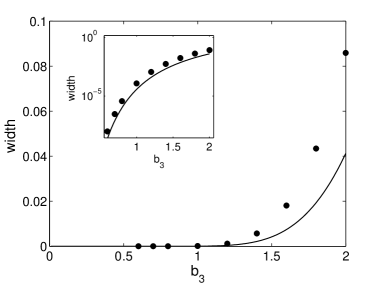
In the bottom panel we show the width of the snaking region as a function of numerically and analytically, where our approximation is in fairly good agreement.
To conclude, we have used variational methods to study the snaking behaviour of localised patterns in the Swift–Hohenberg equation. The approach has several advantages: the exponentially small terms responsible for the phase locking arise naturally in the Lagrangian, giving a simple formula (14) from which the snake and ladder localised states can easily be found, along with their stability. We have concentrated on a simple model equation in the small-parameter regime, but the method is very widely applicable and can be expected to open up a new avenue of research into this challenging field.
References
- (1) D. Bensimon, B. I. Shraiman and V. Croquette, Phys. Rev. A 38, 5461 (1988).
- (2) C. J. Budd and R. Kuske, Physica D 208, 73 (2005).
- (3) J. Burke and E. Knobloch, Phys. Rev. E 73, 056211 (2006).
- (4) J. Burke and E. Knobloch, Phys. Lett. A 360, 681 (2007).
- (5) J. Burke and E. Knobloch, Chaos 17, 037102 (2007).
- (6) A. R. Champneys, Physica D 112, 158 (1998).
- (7) S. J. Chapman and G. Kozyreff, Physica D 238, 319-354 (2009).
- (8) P. Coullet, C. Riera, and C. Tresser, Phys. Rev. Lett. 84, 3069 (2000).
- (9) J.H.P. Dawes, Phil Trans. R. Soc. 368, 3519 (2010).
- (10) G. W. Hunt et al. Nonlinear Dynamics 21, 3 (2000).
- (11) G. Kozyreff and S. J. Chapman, Phys. Rev. Lett. 97, 044502 (2006).
- (12) A. A. Nepomnashchy, M. I. Tribelsky and M. G. Velarde, Phys. Rev. E 50, 1194 (1994).
- (13) Y. Pomeau, Physica D 23, 3 (1986).
- (14) H. Sakaguchi and H.R. Brand, Physica D 97, 274 (1996).
- (15) M. K. Wadee and A. P. Bassom, Proc. R. Soc. Lond. A 455, 2351 (1999).
- (16) M. K. Wadee and A. P. Bassom, J. Eng. Math. 38, 77 (2000).
- (17) M. K. Wadee, C. D. Coman, and A. P. Bassom, Physica D 163, 26 (2002).
- (18) P. D. Woods and A. R. Champneys, Physica D 129, 147 (1999).
- (19) T.-S. Yang and T. R. Akylas, J. Fluid Mech. 330, 215 (1997).