The Physical Model in Action: Quality Control for X-Shooter

Abstract

The data reduction pipeline for the VLT 2^nd generation instrument X-Shooter uses a physical model to determine the optical distortion and derive the wavelength calibration. The parameters of this model describe the positions, orientations, and other physical properties of the optical components in the spectrograph. They are updated by an optimisation process that ensures the best possible fit to arc lamp line positions. ESO Quality Control monitors these parameters along with all of the usual diagnostics. This enables us to look for correlations between inferred physical changes in the instrument and, for example, instrument temperature sensor readings.

1 INTRODUCING X-SHOOTER

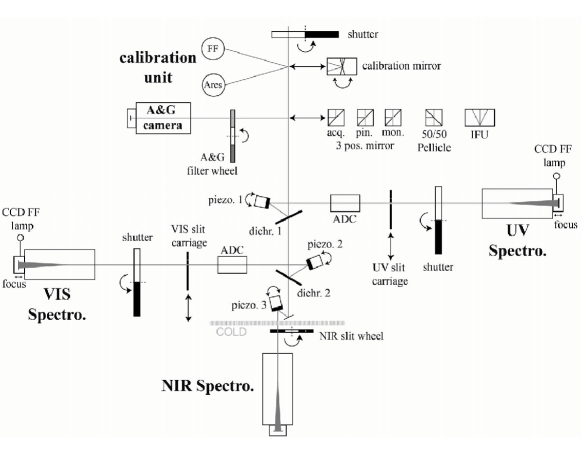
Figure 1: Schematic layout of the X-Shooter instrument. The physical model includes the optical components after the ADC for the UVB and VIS arms and within the cold part of the NIR arm.

X-Shooter[1] is the first of the second generation instruments at the ESO Very Large Telescope (VLT) and has been available since October 1, 2009. It is a medium resolution spectrograph covering the wavelength range of 300–2500 nm in three arms (see Fig 1 for a schematic layout). This allows each arm to be optimised for the wavelength range it covers. The arms are UVB (300–559 nm, $\lambda/\Delta\lambda$ = 5100 for a 1$\stackrel{{{}^{\prime\prime}}}{{}}$ slit), VIS (550–1020 nm, $\lambda/\Delta\lambda$ = 7700 for a 1$\stackrel{{{}^{\prime\prime}}}{{}}$ slit), and NIR (1020–2480 nm, $\lambda/\Delta\lambda$ = 4800 for a 1$\stackrel{{{}^{\prime\prime}}}{{}}$ slit). The separation of light between the arms is achieved with two dichroics. In order to combine large wavelength coverage with medium resolution cross-dispersed echelle spectrographs are used. This results in strongly curved orders with highly tilted lines in each order. The line tilt varies with line position along the order (see Fig. 2 for an example in the VIS arm). Moreover the wavelength ranges of the orders overlap (as usual for echelle spectrographs).

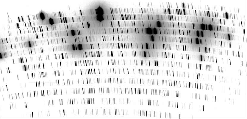
Figure 2: VIS arc line frame. This image illustrates the order curvature and line tilt present in X-Shooter data.

In addition to slits with widths varying from 0$\stackrel{{{}^{\prime\prime}}}{{\vspace*{-0.1ex}.}}$4 to 5$\stackrel{{{}^{\prime\prime}}}{{\vspace*{-0.1ex}.}}$0 and with a common length of 11$\stackrel{{{}^{\prime\prime}}}{{}}$ X-Shooter also offers an Integral Field Unit of 1$\stackrel{{{}^{\prime\prime}}}{{\vspace*{-0.1ex}.}}$8$\times$4$\stackrel{{{}^{\prime\prime}}}{{}}$ that is reformatted by mirrors into 3 slits of 0$\stackrel{{{}^{\prime\prime}}}{{\vspace*{-0.1ex}.}}$6$\times$4$\stackrel{{{}^{\prime\prime}}}{{}}$, which are in turn aligned to form one long slit of 0$\stackrel{{{}^{\prime\prime}}}{{\vspace*{-0.1ex}.}}$6$\times$12$\stackrel{{{}^{\prime\prime}}}{{}}$.

The two optical arms (UVB/VIS) have atmospheric dispersion compensators to reduce the effects of atmospheric refraction on the observations. In order to keep the targets at the same position along the slit for each arm (despite the residual effects of flexure and atmospheric refraction between the guiding wavelength and each arm’s central wavelength) each arm has a piezo controlled mirror. An arc lamp exposure is taken before each observation and the observed positions of a few carefully selected lines are compared to reference positions. The offsets derived from these observations are then compensated for by the piezo-controlled mirrors (Automatic Flexure Control).

The lamps used for calibrations (wavelength calibration arc lamps and flat field lamps) are mounted in the internal calibration unit. All these components (slits, IFU, ADCs, mirror, calibration unit) as well as the acquisition and guiding camera are part of the backbone, which is mounted on the Cassegrain derotator of the telescope.

2 QUALITY CONTROL

Quality Control (QC) in this article refers to the control of data quality. This is part of the end-to-end data flow realized within the ESO VLT, which is extremely important especially for Service Mode (SM) observations. SM observations are flexibly scheduled to match prevailing ambient conditions. For a given observing run, they might be scattered arbitrarily over a given scheduling semester. It is therefore of paramount importance that the instruments used in such observations provide stable and reproducible results. The SM paradigm assumes that if the instrument is healthy and the PI defined constraints are fulfilled for the observation the data will allow the astronomers to perform their scientific studies. The instrument health is monitored mainly by QC using so-called Health Check data, which are processed automatically by dedicated instrument pipelines[2, 3] and which provide so-called QC parameters like the measured central wavelength for a given setting, the detector read-out noise, etc. X-Shooter data are transmitted immediately after acquisition at the VLT to the ESO headquarters at Garching. The calibration part of the data flow is processed in an incremental pattern, once per hour. Quality information is fed back to Paranal and reviewed to allow a very quick detection of possible problems.

Some Health Check data and parameters are of course very instrument dependent, while others, like detector related parameters, may be common across several instruments. For spectrographs the stability and reproducibility of the wavelength scale is one of the most important aspects. Other parameters include instrumental efficiency, stability of calibration lamps (to avoid underexposed data as well as saturated ones), and detector parameters (e.g. detector read-noise and presence of structure and/or patterns).

Fig. 3 shows a striking example of the usefulness of such health check parameters. Here the structure along the y-axis is shown for the fast, low gain readout of the X-Shooter VIS CCD. On March 6, 2010 (JD 2455262) a strong interference pattern showed up for this readout mode, which an be clearly seen in the plot as the data points above 1. While the engineers managed to reduce the amplitude of this pattern to a level where it is hard to see looking at the data, the elevated level of the structure parameter still indicates its presence.

Figure 3: The structure along the y-axis of the X-Shooter VIS CCD vs. time. The sudden strong increase marks the presence of an electronic interference pattern, which - albeit much reduced - persists until today.

3 PHYSICAL MODEL VS. PATTERN MATCHING

One of the main challenges for automatic data processing is the correct identification of observed features like arc lines or photometric standard stars. Here one can distinguish between two principal approaches: pattern matching and physical model. Pattern matching relies, as the name already suggests, on the detection of patterns (e.g. groups of standard stars, groups of arc lines) to correctly identify the observed features. This approach requires only a rough idea of the instrumental characteristics (e.g. pixel scale, dispersion, wavelength range) and allows to treat a large variety of observations and instrumental configurations with the same pipeline. It is therefore especially well suited to multi-mode instruments (e.g. FORS2[3]) and/or not very stable instruments. In the case of FORS2 it has been shown that this approach works extremely well and allows to process almost all of the multi-object spectroscopic data[4]. As an impressive example, tests showed that – after adjusting the header keywords to resemble FORS2 data – the FORS2 pipeline processes multi-object spectroscopy data from the Low-Resolution Spectrograph at the Hobby-Eberly Telescope without problems. So the pattern matching indeed provides very versatile routines. The disadvantage of this approach is that the cause for a change in the observed data cannot easily be identified. Fig. 4 shows the central wavelength of a specific long-slit setup for FORS2. Obviously the central wavelength varies with time, but to identify the change in temperature as the underlying cause was not trivial. And it still does not tell whether the temperature affects the slit position or the grism properties or both. The pattern matching also reaches its limits in spectroscopy if there are large gaps between arc lines and/or the edges of the nominal wavelength range are not covered by arc lines.

Figure 4: The central wavelength of GRIS_300V for the 0.3$\stackrel{{{}^{\prime\prime}}}{{}}$ wide long-slit in FORS2 vs. time (left) and vs. focus temperature (right).

The physical model approach, on the other hand, relies on detailed instrument knowledge and an appropriate implementation of that knowledge in a pipeline. In this case the observed data are described by a set of functions derived from the optical description of the instrument (including the refractive indices of prisms etc.) and a change in observed data may therefore more easily be traced back to a change in instrument components. An additional advantage of the physical model approach is that deficiencies in the calibration data may be counterbalanced (e.g. a lack of arc lines in certain spectral regions). Also distortions can be much better described in such an approach than with a standard polynomial fit, because they do not depend in such a simple way on detector coordinates. Moreover the polynomials often have boundary problems in the extreme areas (like the edges of the field-of-view). The physical model is also extremely well suited for the processing of echelle data, where the order overlap requires that lines observed at rather different positions on the detector are correctly assigned the same wavelength. While this often causes problems in the classical polynomial fitting, where each order is treated independently, the overall optimisation of the physical model allows a comprehensive treatment of all lines simultaneously.

The physical model approach[5] was employed with great success for the Space Telescope Imaging Spectrograph (STIS[6, 7]) onboard the Hubble Space Telescope. Independently ESO first adopted this approach for the UV-Visual Echelle Spectrograph (UVES) in 2000[8]. Its pipeline uses a physical model to predict and verify the spectral format and to allow robust and automatic wavelength calibration for a virtually infinite number of instrument settings (the central wavelengths of its independent blue and red arms can be set arbitrarily within certain limits). At the time of the UVES pipeline development and commissioning, the annealing functionality was not as advanced, accurate, and reliable as it is now, thus in case of large instrument shifts (e.g. caused by earthquakes), the operational scenario requires a re-alignment of the instrument to a reference position using reference spectral format check frames.

The physical model approach was then once more realized in the pipeline for the CRyogenic high-resolution InfraRed Echelle Spectrograph (CRIRES[9]), where it is especially useful due to the limited coverage in wavelength per detector, which can result in calibration data containing only one or even no arc lines on a particular detector. X-Shooter is thus the third ESO instrument for which a physical model is used in the automatic data processing. In its pipeline[2] – if used in physical model mode – the model is used in most of the data reduction steps (except master bias, dark and flat generation), including science data processing.

4 THE X-SHOOTER PHYSICAL MODEL

The X-Shooter Physical Model (hereafter XPM) is a series of matrix transformations, each representing an optical surface in the spectrograph as specified in the Zemax optical design. This enables the physically based computation of the wavelengths associated with each detector pixel in a given exposure based on a four-dimensional vector containing the three spatial coordinates and the wavelength.

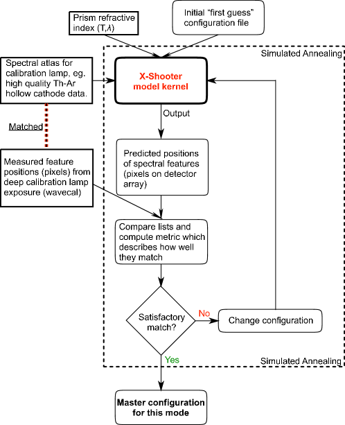
Figure 5: The optimisation process of the physical model.

The central part of the XPM is a ray trace (referred to here as the “model kernel”) that approximates the optical path of the three X-Shooter spectrograph arms. Given a wavelength, echelle order and a position along the slit, the model kernel will return the location at which the detector is illuminated.

The model kernel is a simplified ray trace of the X-Shooter spectrograph arms, based upon the optical design with the initial values of many parameters taken directly from the X-Shooter Zemax files. The simplification is necessary in order allow many iterations of the model kernel both during the optimisation process or in some of the higher level functions. Due to the similarity of the arms we are able to use essentially the same model structure for all three arms.

The model kernel uses a parametrisation of the relative positions and orientations of the principal dispersive optical components (e.g. prisms) of the three X-Shooter arms. We use exposures of wavelength calibration sources (ThAr for UVB and VIS, ArKrNeXe penray lamps for NIR), identify the locations on the detector of known wavelengths and run an optimisation algorithm that finds the combination of XPM parameter settings that is best able to place those wavelengths at the observed positions. Figure 5 provides a schematic overview of the optimisation process. As the optimisation process is sensitive to false matches, we use customized line catalogs that provide unblended lines at the X-Shooter spectral resolution. Since the physical model needs fewer arc lines than the polynomial approach the cleaning of the line lists proved to be uncritical.

Once optimised in this way, the XPM and the accompanying parameter configuration can be used to calibrate science exposures since the wavelength associated with each pixel can be interpolated via iterative executions of the model kernel. Moreover, as part of routine operations, we continually re-optimise the XPM parameter configuration. Obviously this gives us the most contemporaneous calibration to apply to science data, and in addition it enables us to monitor how the physical parameters of the instrument change.

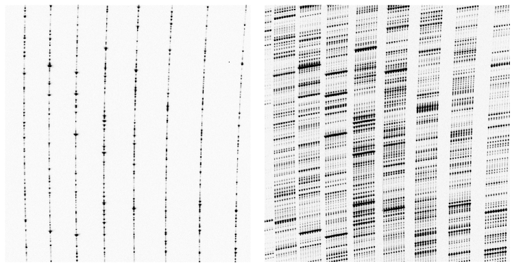
Figure 6: UVB example of 1-pinhole (left) and 9-pinhole (right) data

The configuration files (one per arm) contain the following parameters (number of parameters per arm in brackets). Fixed parameters are marked by slanted font:

• temperature of prism(s) (read from header, 1 for UVB and VIS, 3 for NIR)

• orientation of entrance slit and detector plane along three axes (6)

• orientation of prisms, for both entrance and exit surface, along three axes (6 for UVB and VIS, 18 for NIR)

• orientation of grating along three axes (3) and grating constant (1)

• location of the center of the pixel array along 2 axes and of the central pinhole/slit center (2$+$2)

• relative positions of the pinholes along the slit (8)

• focal length of camera and collimator (2)

• slit scale (1)

• magnitude and wavelength zeropoint for chromatic aberration correction (2 for UVB and VIS)

• additional tilt of primary NIR prism (1 for NIR)

• pixel size (1)

• detector rotation (1, only important for more than one detector per arm)

• 2^nd order distortion coefficients

• refractive indices of the prisms (1 each for UVB [Silica] and VIS [Schott SF6], 2 for NIR [Infrasil and 2$\times$ZnSe])

The fact that the prism temperatures are read from the headers allows to adjust a configuration derived from daytime calibrations to science data (and/or flexure compensation data) observed at night.

Figure 7: The fitted focal length of the UVB spectrograph camera vs. the focus temperature used to adjust it. The line is not a fit to the data, but shows the relation used to mechanically adjust the focus (see text for details).

5 APPLYING THE PHYSICAL MODEL

We concentrate here on regular daytime calibration exposures obtained with the telescope parked at Zenith (i.e. with the three spectrographs in their null flexure position) and what they tell us about physical parameters changing as a function of epoch and environmental conditions. In a separate paper[10] we present a similar analysis of physical parameters as a function of instrument orientation.

Ultimately the goal of this work is firstly to gain some insight into how the spectrographs change physically over time and secondly to be able to predict changes in physical parameters as a function of environmental conditions. This would allow the calibration to take into account the fact that the environmental conditions at the time of science exposures will often differ from those at the time of day time calibrations.

Figure 8: The fitted orientation of the entrance surfaces of the first and third prism in the NIR arm vs. time (left) and vs. each other (right).

We use two types of X-Shooter calibrations to fine-tune the physical model during normal operations (see Fig. 6 for examples): 1-pinhole data (a.k.a. formatcheck) and 9-pinhole data (a.k.a. wave or 2dmap). About 40 such observations have been taken since start of operations (October 1, 2009) for each arm and data type. The 1-pinhole data are used to verify the overall format of the data. Fitting these data the following parameters may be modified: location of the central pinhole and of the central detector pixel, grating constant, focal length of the camera, tip-tilt of all prisms (both entrance and exit surfaces), orientation of the grating and of the detector plane. If one fits the 9-pinhole data also the slit scale, the orientation of the entrance slit and the focal length of the collimator may be varied.

In standard operations the parameter ranges are chosen so that they are large enough to encompass any realistic physical changes over time (in the absence of interventions or earthquake damage) but small enough that the optimisation can be expected to converge without a prohibitively high number of iterations. The ranges in use have been established from an initial physically motivated estimate modified by trial and error. An example of this is that we found that larger than expected ranges were required for UVB 1-pinhole data, most likely due to a not fully corrected temperature dependency. This process is ongoing, and as we whittle down the number of open parameters we will be less constrained by the optimisation time. To give an order of magnitude, a typical parameter range is $\pm$0.1mm for the focal distance of the VIS collimator (or $\approx$0.02%) .

Figure 7 shows a good example of correlations found with the physical model. The focus of the UVB camera is known to be quite sensitive to temperature. It is therefore mechanically adjusted automatically by 10.9$\mu$m per degree Celsius. The physical model clearly finds exactly that correlation when fitting the data. The nature of the 5 data points in the top right is unfortunately not yet clear to us.

Due to the large number of parameter that are allowed to vary during the optimisation we also sometimes encounter degenerate parameters. Fig. 8 shows an example for such a degeneracy with the orientation of the entrance surfaces of the first and third prism in the NIR arm varying in step. In such cases the algorithm finds a marginally better fit with varying two parameters, which compensate each other to some degree. Such degeneracies are hard to break with the current data set, which have for instance the same flexure in all data. In a related paper[10] we describe efforts to reduce the number of free parameters using flexure compensation observations.

6 SUMMARY

The physical model used in the X-Shooter pipeline has proven to provide an accurate description of the instrument, which allows to process the vast majority of data without problems. In addition it provides us with information on the status of the various optical instrument components and how that status changes with time and temperature. Analysis of the currently available set of calibration data has revealed some degeneracy amongst the physical model parameters being optimised. The next step will be to try to determine a reduced set of parameters that is free of degeneracy. The expectation is that this will reveal more robust correlations, moreover the accumulation of data over time will improve the signal to noise in the dataset.

- [1] Kaper, L., D’Odorico, S., Hammer, F., Pallavicini, R., Kjaergaard Rasmussen, P., Dekker, H., Francois, P., Goldoni, P., Guinouard, I., Groot, P. J., Hjorth, J., Horrobin, M., Navarro, R., Royer, F., Santin, P., Vernet, J., and Zerbi, F., “X-Shooter: A Medium-resolution, Wide-Band Spectrograph for the VLT,” in [Science with the VLT in the ELT Era ], A. Moorwood, ed., 319 (2009).
- [2] Modigliani, A., Goldoni, P., Francois, P., Guglielmi, L., Haigron, R., Royer, F., Horrobin, M., Bristow, P., Ballester, P., Moehler, S., and Vernet, J., “The X-Shooter pipeline,” in [Observatory Operations: Strategies, Processes, and Systems III ], D. R. Silva, A. B. Peck & B. T. Soifer, ed., Proc. SPIE 7737 (2010).
- [3] Izzo, C., Y., J., and P., B., “A Bottom-Up Approach to Spectroscopic Data Reduction,” in [The 2007 ESO Instrument Calibration Workshop ], A. Kaufer & F. Kerber, ed., 191 (2008).
- [4] Moehler, S., “Good News for MOS, MXU & Co. - The New Spectroscopic Pipeline for the FORSes,” in [The 2007 ESO Instrument Calibration Workshop ], A. Kaufer & F. Kerber, ed., 87 (2008).
- [5] Ballester, P. and Rosa, M. R., “Modeling echelle spectrographs,” A&AS 126, 563 (1997).
- [6] Bristow, P., Kerber, F., and Rosa, M. R., “STIS Calibration Enhancement: Wavelength Calibration and CTI,” in [The 2005 HST Calibration Workshop: Hubble After the Transition to Two-Gyro Mode ], A. M. Koekemoer, P. Goudfrooij, & L. L. Dressel, ed., 299 (2006).
- [7] Kerber, F., Bristow, P., and Rosa, M. R., “STIS Calibration Enhancement (STIS-CE) : Dispersion Solutions Based on a Physical Instrument Model,” in [The 2005 HST Calibration Workshop: Hubble After the Transition to Two-Gyro Mode ], A. M. Koekemoer, P. Goudfrooij, & L. L. Dressel, ed., 309 (2006).
- [8] Ballester, P., Modigliani, A., Boitquin, O., Cristiani, S., Hanuschik, R., Kaufer, A., and Wolf, S., “The UVES Data Reduction Pipeline,” The Messenger 101, 31 (Sept. 2000).
- [9] Bristow, P., Kerber, F., and Rosa, M. R., “Model Based Instrument Calibration,” in [The 2007 ESO Instrument Calibration Workshop ], A. Kaufer & F. Kerber, ed., 199 (2008).
- [10] Bristow, P., Kerber, F., Vernet, J., Moehler, S., and Modigliani, A., “Using the X-shooter physical model to understand instrument flexure ,” in [Ground-based and Airborne Instrumentation for Astronomy III ], I. S. McLean, S. K. Ramsay, & H. Takami, ed., Proc. SPIE 7735 (2010).