Nonparametric Bayesian multiple testing for longitudinal performance stratification
Abstract
This paper describes a framework for flexible multiple hypothesis testing of autoregressive time series. The modeling approach is Bayesian, though a blend of frequentist and Bayesian reasoning is used to evaluate procedures. Nonparametric characterizations of both the null and alternative hypotheses will be shown to be the key robustification step necessary to ensure reasonable Type-I error performance. The methodology is applied to part of a large database containing up to 50 years of corporate performance statistics on 24,157 publicly traded American companies, where the primary goal of the analysis is to flag companies whose historical performance is significantly different from that expected due to chance.
doi:
10.1214/09-AOAS252keywords:
.T1Supported by a graduate research fellowship from the U.S. National Science Foundation.
1 Introduction
1.1 Multiple testing of time series
Suppose a single time series of length is observed for each of different units. Two possible models for each time series are entertained: a simple autoregressive null model and a more complex alternative model . The goal is to determine which units come from the alternative model.
This is a common problem in the analysis of multiple time series, and although many details will be context-dependent, certain common themes emerge. Of key interest is how, in repeatedly applying a procedure used for testing a single time series, the rate of Type-I errors can be controlled. Model-based approaches are an attractive option, but model errors can become overwhelming in the face of massive multiplicity. One of this paper’s main results is that great care must be taken in characterizing and in order to keep false positives at bay, with the suggested robustification step involving the use of nonparametric Bayesian methods.
In typical hypothesis-testing scenarios involving standard parametric models and , the Bayes factor contains an “Ockham’s razor” term [Jefferys and Berger (1992)] that penalizes the more complex model. In most cases this is the result of needing to integrate the likelihood across a higher-dimensional prior under the more complex model, which will therefore have a more diffuse predictive distribution. This penalty for model complexity is quite different from any sort of penalty term imposed for conducting multiple hypothesis tests [Scott and Berger (2008)].
But the multiple-testing framework employed here uses Dirichlet-process mixtures to represent the unknown null and alternative models, which are properly thought of as being infinite-dimensional. Another of this paper’s main objectives is to clarify the nature and operating characteristics of this penalty for model complexity in nonparametric settings—specifically, how it interfaces with the recommended multiple-testing methodology.
1.2 Motivating example
A running example from management theory will be used to motivate and study the proposed Bayesian model. The results and discussion are problem-specific, but areas in which the methodology and lessons can be generalized will be pointed out.
Our data set covers up to 50 years of annual performance (operationalized by a common accounting measure) for over 24,000 publicly traded American companies. The goal of the analysis is to flag firms whose performance is highly unlikely to have occurred by random chance, since these firms may have good (or bad) management practices that are discernible through follow-up case studies.
Longitudinal performance stratification is a classic topic in management theory. Indeed, one of the primary aims of strategic-management research, and the conceit of many best-selling books, is to explain why some firms fail and others succeed.
Much academic work in this direction focuses on decomposing observed variation into market-level, industry-level and firm-level components[Bowman and Helfat (2001), Hawawini, Subramanian and Verdin (2003)]. Of the work that attempts to identify specific nonrandom performers, much of it relies upon model-free clustering algorithms [e.g., Harrigan (1985)], which contain no guarantee that the clusters found will be significantly different from one another. Other approaches employ simple classical tests [Ruefli and Wiggins (2000)], often based upon ordinal time series. These have the advantage of being model-free, but are typically not based upon sufficient statistics, and suffer from the fact that available multiplicity-correction approaches (e.g., Bonferroni correction) tend toward the overly aggressive.
Due to the number of firms for which public financial data is available, this problem makes an excellent testbed for the study of general-purpose multiple-testing methodology in time-series analysis. There is, however, no theoretical ideal of what an “average-performing” company should look like, beyond the notion that it should revert to the population-level mean even if it has some randomly good or bad years. The Bayesian approach requires that suitable notions of randomness and nonrandomness be embodied in a statistical model. This model must confront an obvious multiplicity problem: many thousands of companies will be tested, and false positives will make expensive wild-goose chases out of any follow-up studies seeking to explain possible sources of competitive advantage. Robustness and trustworthy Type-I error characteristics are therefore crucial practical considerations, and so even though this paper’s modeling approach is Bayesian, it also contains much frequentist reasoning regarding Type-I error rates.
2 Testing a zero-mean AR(1) model
2.1 The model
This section outlines a basic framework for multiple testing that, for the sake of illustration, will be purposely simplistic. Nonetheless, it will provide a useful jumping-off point for the methodological developments of subsequent sections, and will show why more flexible models are typically needed in order to achieve reasonable Type-I error performance.
Let be the observation for unit at time , and let be the vector of observations for unit . In the management-theory example, is a standardized performance metric called Return on Assets (ROA), which measures how efficiently a company’s assets generate earnings. Each company’s ROA values were regressed upon a set of covariates judged to be relevant by three experts in management theory collaborating on the project. These include the company’s size, debt-to-equity ratio and market share, along with categorical variables for year and for industry membership. [See Ruefli and Wiggins (2002), for a summary of the literature regarding covariate effects on observed firm performance.] The actual values used in the following analyses were the residuals from this regression. Also, since the question at issue is one of relative performance, not absolute performance, these residuals were standardized by CDF transform to follow a distribution.
Since we do not expect random gains or losses in one year to be completely erased by the following year, a model accounting for serial autocorrelation seems mandatory. Management-theoretic support for this assumption in the present context can be found in Denrell (2003) and Denrell (2005); analogous situations in engineering, finance and biology are very common.
The null hypothesis is then a stationary AR(1) model depending upon parameter :
This assumption allows for long runs of good or bad performance due simply to chance: a large shock () may take quite awhile to decay depending upon the value of , which is assumed to lie on .
Nonnull companies can then be modeled as AR(1) processes that revert to a nonzero mean. Placing a mixture prior on this unknown mean will then encode the relevant hypothesis test:
| (1) | |||||
| (2) | |||||
| (3) |
with is the vector of all ones, is the familiar AR(1) variance matrix, is a point mass at 0, and is the prior probability of arising from the alternative hypothesis. The exchangeable normal prior on the nonzero means reflects the prior belief that, among firms that systematically deviate from zero, most of the deviations will be relatively small.
The posterior probabilities then can be used to flag nonnull units. In some contexts, these are called the posterior inclusion probabilities, reflecting inclusion in the “nonnull” set.
The model must be completed by specifying priors for , and . In the example at hand, the data have been standardized to a scale, so it makes sense to choose . In more general settings, the prior for must be appropriately scaled by and in the absence of strong prior information, since the marginal variance of the residual autoregressive process is the only quantity that provides a default scale for the problem.
The conditional likelihoods of each data vector under the two hypotheses ( versus ) are available in closed form:
| (4) | |||||
| (5) |
where is the matrix of all ones.
2.2 Bayesian adjustment for multiplicity
Multiplicity, from a Bayesian perspective, is handled through careful treatment of the prior probability .
One possibility is to choose a small value of , with the expectation that a prior bias in favor of the null will solve the problem. But the key intuition in using this model for multiple testing is to treat as just another model parameter to be estimated from the data, giving it a uniform prior. This induces an effect that is often referred to as an automatic multiple-testing penalty, with the effect being “automatic” in the sense that no arbitrary penalty terms must be specified.
This effect can most easily be seen if one imagines repeatedly testing a fixed number of signals in the presence of an increasing number of null units. Asymptotically, the posterior mass of will concentrate near , making it increasingly difficult for all units (even the signals) to overcome the prior belief in their irrelevance. This yields much the same effect as choosing a small value for after the fact, but Bayesian learning about negates the need to make such an arbitrary choice.
Two caveats are in order. First, this should not be misinterpreted as saying that Bayesians need never worry about multiplicities. Automatic adjustment depends upon allowing the data itself to choose , and more generally, upon careful treatment of prior model probabilities. The adjustment itself can be seen primarily in the inclusion probabilities, and will not necessarily be incorporated into other posterior quantities of interest. In particular, the joint distribution of effect sizes, conditional on their being nonzero, will fail to adjust for multiplicity.
Second, it is still necessary to choose a threshold on posterior probabilities in order to get a decision rule about “signal” versus “noise.” An obvious threshold is , but ideally this threshold should be chosen to minimize Bayesian expected loss under properly specified loss functions. Perhaps, for example, the loss incurred by a false positive is constant while the loss incurred by a false negative scales according to some function of the underlying difference from . Introducing such loss functions will complicate the analysis only slightly, without changing the fundamental need to account for multiplicity.
It is important to distinguish this fully Bayesian model from the empirical-Bayes approach to multiplicity correction, whereby is estimated by maximum likelihood [see, e.g., Johnstone and Silverman (2004)]. These two approaches are intuitively similar, since the prior inclusion probability is estimated by the data in order to yield an automatic multiple-testing penalty. Yet the approaches have quite different operational and theoretical properties [Scott and Berger (2008)], with the focus here being on the fully Bayesian approach.
Similar multiple-testing procedures have been extensively studied in many different contexts. See Scott and Berger (2006) for theoretical development; Do, Muller and Tang (2005) for genomics; Scott and Carvalho (2008) and Carvalho and Scott (2009) for portfolio selection; and George and Foster (2000) and Cui and George (2008) for examples in regression.
The posterior inclusion probabilities can be computed straightforwardly using importance sampling to account for posterior uncertainty about , and , which will be stable as long as is not too close to or . The advantage of importance sampling here is that a common importance function may be used for all marginal inclusion probabilities, greatly simplifying the required calculations. After transforming all variables to have unrestricted domains, importance sampling was used to compute the results presented in this section, with repetition and plots of the importance weights used to confirm stability.
2.3 Results on ROA data
Historical ROA time series for 3459 publicly traded American companies between 1965 and 2004 were used to fit the above model. This encompasses almost every public company over that period for which at least 20 years of data were available. Standard independent conjugate priors for and were used:
| (6) | |||||
| (7) |
where indicates that the normal prior for is truncated to lie on . These priors were chosen to reflect the expectations of the collaborating management theorists regarding the persistence and scale of random ROA fluctuations from year to year. Because these parameters appear in both the null and alternative models, integrals over these priors appear in both the numerator and denominator of the Bayes factor comparing versus , making them not overly influential in the analysis; see Berger, Pericchi and Varshavsky (1998) for general guidelines on choosing common hyperparameters in model-selection problems.
In many cases the results of the fit seemed reasonable. Most firms were assigned to with high probability, while companies with obvious patterns of sustained excellence or inferiority were flagged as being from with very high probability. Figure 1 contains instructive examples: two excellent companies (WD-40 and Coca-Cola), along with one obviously poor company (Oglethorpe Power), were assigned greater than probability of being nonnull. A fourth example, Texas Intruments, had several intermittent years of good performance but no pattern of sustained excellence, and the model gave it greater than probability of being from the null model.


On the other hand, the model displayed two serious shortcomings:
- •
-
•
More subtly, the model imposed a homogeneous error structure on data that seemed rather heterogeneous. Some fairly basic exploratory data analysis indicated that firms displayed differing degrees of “stickiness” in their trajectories. This suggested that a single value of for the entire data set might be unsatisfactory. Likewise, some firms appeared systematically more volatile than others, making a single-variance model equally questionable.
2.4 Robustness simulations
The possibility of model errors in (1)–(3) bring the issue of robustness to the forefront. This section describes the results of a simulation study that shows just how poorly this model can perform when a particular type of model error is encountered: deviation from the “single , single ” approach to describing the AR(1) residuals of all companies in the sample.
Several data sets displaying different levels of heterogeneity were simulated. The homogeneous (i.e., single , single ) model was subsequently fit to each simulated data set in order to assess the robustness of the procedure’s Type-I error performance.
Each simulated data set had 3500 times series of length , with each time series drawn from a mixture distribution of AR(1) models. These distributions ranged from trivial one-component mixtures (for which the assumed model was true) to complex nine-component mixtures (for which the assumed model was quite a bad approximation). These conditions are summarized in Table 1. In the four- and nine-component models, all components were equiprobable. Since all simulated companies had , ideally there should be no positive flags.
For the purposes of classification, thresholding is reported at the and the levels, where is the posterior inclusion probability for company . The first () threshold reflects a 0–1 loss function that symmetrically penalizes false positives and false negatives. The second threshold is arbitrary, but meant to reflect a more conservative approach to identifying signals. A full decision-theoretic analysis incorporating more realistic loss functions would yield a different, data-adaptive threshold.
Table 1 supports two conclusions:
-
•
The proposed model yields very strong control over false positives when its assumptions are met: 3 false positives and 0 false positives in the two cases investigated, out of 3500 units tested. This confirms that the theory outlined in Scott and Berger (2006), which concerns the much simpler normal-means testing problem, applies here as well.
-
•
This excellent Type-I error profile is not at all robust to a violation of the autoregressive model’s assumptions. In the most extreme case, nearly a third of units (1045 out of 3500) tested had inclusion probabilities , when in reality none were from the alternative model. In other less extreme cases, the false positives still numbered in the hundreds, which is clearly unsatisfactory.
| Number of components: Model | # | # | |
|---|---|---|---|
| 1: | 0.01 | ||
| 1: | 0.02 | ||
| 4: | 0.02 | ||
| 4: | 0.08 | ||
| 9: | 0.37 | ||
| 9: | 0.29 |
These results dramatically illustrate the effect of heterogeneity in the autoregressive profiles of each tested unit. If such heterogeneity exists but is ignored, the Type-I error performance of the procedure may be severely compromised.
3 A nonparametric null model
In the previous section, a specific form of model error—different groups of companies following different AR models—was shown to be a source of overwhelming Type-I errors. Hence, a natural extension is to consider a more complicated autoregressive model for the residuals that accounts for the possibility of stratification.
The Dirichlet process [Ferguson (1973)] offers a straightforward nonparametric technique for accommodating uncertainty about this random distribution. Let represent the response vector for unit , for now ignoring any contribution due to a nonzero mean. Recall that for parameter , denotes the AR(1) variance matrix. The DP mixture model can then be written as a hierarchical model:
| (8) | |||||
| (9) | |||||
| (10) |
where the hyperparameters and must be chosen to reflect the expected properties of the base measure (which is a product of two independent distributions, a normal and an inverse-gamma), and where controls the degree of expected departure from the base measure.
Dirichlet-process priors for nonparametric Bayesian density estimation were popularized by Ferguson (1973), Antoniak (1974), and Escobar and West (1995). An example of their use in analyzing nonlinear autoregressive time series can be found in Müller, West and MacEachern (1997).
Realizations of the Dirichlet process are almost surely discrete distributions, and so we expect some of the ’s to be the same across companies. This is the DP framework’s primary strength here, since it will facilitate borrowing of information across time series. Simply allowing each time series to have its own and own would make for a simpler model (albeit with more parameters), but the DP prior reflects the subject-specific knowledge that significant clustering of autoregressive parameters should be expected.
This will lead to behavior similar to that predicted by a finite mixture of AR(1) models, such as the kind considered by Frühwirth-Schnatter and Kaufmann (2008). The Dirichlet-process prior, however, avoids the complicated task of directly computing marginal likelihoods for mixture models of different sizes, and so makes computation much simpler. Note that since the marginal distribution of one draw from a Dirichlet-process mixture depends only on the base measure, the DP acts like a mixture model that is predictively matched to a single observation.
It is important to consider, of course, how choices for and affect the implied prior distributions both for the number of mixture components and for the parameters associated with each component. The marginal prior for the parameters of each mixture component is simply given by the base measure, while the prior for can be described in terms of and , the desired number of mixture components, using results from Antoniak (1974).
4 A nonparametric alternative model
4.1 Trajectories as random functions
Section 2 considered a simple constant-mean AR(1) model for nonnull units, and Section 3 modified the AR(1) assumption to account for a richer autoregressive structure. This section now modifies the constant-mean assumption to allow for time-varying nonzero trajectories upon which the autoregressive residuals are superimposed. Most management teams, after all, do not stay the same for 40 or 50 years, and we should not expect their performance to stay the same, either.
Firm performance trajectories can be viewed as continuous random functions that are observed at discrete (in this case, annual) intervals. This is essentially a nonparametric version of a mixed-effects model for longitudinal data [Kleinman and Ibrahim (1998)]. Recent examples of such models include Bigelow and Dunson (2005), Dunson and Herring (2006), and, in a spatial context, Gelfand, Kottas and MacEachern (2005).
Let be a continuous-time stochastic process for each observed unit, and let denote the vector of times at which each unit was observed. Then the model is
| (11) | |||||
| (12) | |||||
| (13) |
where is the nonparametric residual model defined in Section 3, represents a point mass at the zero function , and is a random distribution over a function space . As in Section 2, is the unknown prior probability of coming from the alternative model , represented in this case by the distribution . It is convenient to represent each hypothesis test using a model index parameter : if (i.e., the null model is true for unit ), and otherwise.
4.2 Choice of features for
The crucial consideration in using the above model for hypothesis testing is that the space from which each is drawn must be restricted to a sufficiently small class of functions. This would be necessary even if were only being estimated, and not tested against a simpler model: if is too broad, then the alternative model itself will not be likelihood-identified, since any pattern of residuals could equally well be absorbed by the mean function.
But this guideline is even more important in model-selection problems; an over-broad class of functions will mean that the random distribution is vague, in the sense that the predictive distribution of observables will be diffuse. It is widely known that using vague priors for model selection can be produce very misleading results, and will typically have the unintended consequence of sending the Bayes factor in favor of the simpler model to infinity. This is often known as Bartlett’s paradox in the simple context of testing normal means [Bartlett (1957)], but the same principle applies here.
It may also be the case that elements of depend upon some parameter . Since this parameter appears only in the alternative model, needs a proper prior, or else the marginal likelihoods will be defined only up to an arbitrary multiplicative constant.
Similar challenges occur in all model-selection problems. General approaches and guidelines for choosing priors on nonshared parameters can be found in Laud and Ibrahim (1995), O’Hagan (1995), Berger and Pericchi (1996), and Berger, Pericchi and Varshavsky (1998). But very few tools of analogous generality have been developed for nonparametric problems, with most work concentrating on how to compute Bayes factors for pre-specified models [Basu and Chib (2003)], or how to test a parametric null against a nonparametric alternative of a suitably restricted form [Berger and Guglielmi (2001)].
This leaves just two obvious criteria for choosing and in the face of weak prior information:
-
1.
Elements of should be smooth, that is, slowly varying on the unit-time scale of the residual model. This will allow deconvolution of the mean process from the residual, and reflects the prior belief that the mean function will describe long-term departures from in the face of short-term autoregressive jitters. (Indeed, these departures are precisely what the methodology is meant to detect.)
-
2.
should be centered at the null model, and should concentrate most of its mass on elements of that predict values on a scale similar to those predicted by the null model. This will avoid Bartlett’s paradox, and generalizes the argument made by Jeffreys (1961) in recommending an appropriately scaled Cauchy prior for testing normal means.
These criteria allow much wiggle room, but at least provide a starting point. Unfortunately there is no objective solution, in this or in any model-selection problem, though the closest thing to a default approach is to simply choose the marginal variance of the alternative process to exactly match the marginal variance of the null process. Best, of course, is to conduct a robustness study, where the features of the nonparametric alternative not shared by the null are varied in order to assess changes in the conclusions. This will usually be quite difficult in large multiple-testing problems, since computations for just a single version of the alternative model may be expensive.
The choice of , the precision parameter for the residual Dirichlet-process prior, is relatively free by comparison, since this parameter appears in both the null and alternative models. Strictly speaking, in order to use anoninformative prior for , verification of the conditions inBerger, Pericchi and Varshavsky (1998) regarding group invariance is necessary, which is difficult in this case. (The issue is that a parameter does not necessarily mean the same thing in both and just because it is assigned the same symbol in each.) In the absence of a formal justification for using a noninformative prior, the conservative approach is to elicit priors for in terms of the expected number of AR(1) mixture components in each of and . Often there will be extrinsic justification for choosing to be the same under both models.
5 A model for the corporate-performance data
5.1 Model details
As an example of how tests involving (11)–(13) can be constructed, this section outlines a nonparametric model for a larger subset of the corporate-performance data containing 5498 firms. This contains every publicly traded American company between 1965 and 2005 for which at least 15 years of history were available.
The class of Gaussian processes with some known covariance function is ideally suited for modeling nonzero trajectories, since the covariance function can be chosen to yield smooth functions with probability 1, and since the prior marginal variance of the process can be controlled exactly (so that Bartlett’s paradox may be easily avoided). Gaussian processes have the added advantage of analytical tractability, which is very important in hypothesis testing because of the need to evaluate the marginal likelihood of the data under the alternative model. More general classes of functions are certainly possible, though perhaps computationally challenging in the face of massive multiplicity.
One additional feature to account for is clustering, since management theorists are interested in identifying a small collection of archetypal trajectories that may correspond to different sources of competitive advantage. Partitioning of firms into shared trajectories is especially relevant for advocates of the so-called “resource-based view” of the firm [Wernerfelt (1984)]. Additionally, clustering on treatment effects is known to increase power in multiple-testing problems [Dahl and Newton (2007)].
The approach considered here is similar to that introduced byDunson and Herring (2006). The distribution of nonzero random functions is modeled with a functional Dirichlet process:
| (14) | |||||
| (15) |
The functional Dirichlet process in (14) has precision parameter and is centered at a Gaussian process with covariance function . At time , the value of the function has a Dirichlet-process marginal distribution: , where . In choosing the hyperparameter , close attention must be paid to the marginal variance of the residual model, so that variance inflation in (15) does not overwhelm the Bayes factor. For greater detail on Gaussian processes for nonparametric function estimation, see Rasmussen and Williams (2006).
This model is significantly richer than the simplistic framework developed in Section 2, but is similar in two crucial ways:
-
Centering at the null model,
since the Gaussian process in (15) leads to . As before, it is equally likely a priori that a firm’s trajectory will be predominantly negative or predominantly positive.
- Variance inflation
The model also solves both of the major problems encountered in the ROA data: time-varying nonzero trajectories, and clustering both of trajectories and of company-specific parameters for the autoregressive residual.
An extensive prior-elicitation process was undertaken with three experts in management theory who had originally compiled the data. For the base measure of the Dirichlet-process mixture of AR(1) covariance models, the same hyperparameters from the parametric model in (6) and (7) were used. Hence, the starting point for this elicitation was , which is the prior marginal variance of the residual AR process (assessed by simulation), and (on a 41-year time scale), which reflected the experts’ judgments about the long-term effects of strategic choices made by firms. The elicitees were repeatedly shown trajectories drawn from this prior and other similar priors, and soon settled upon and as values that better reflected their expectations. Additionally, they chose , and on the basis of how many clusters they expected.
For the actual data, a third trajectory model was also introduced: a DP mixture of constant trajectories rather than of Gaussian-process trajectories. This entails only a slight complication of the analysis, in that now (13) is a three-component mixture rather than a two-component mixture. This is equivalent to including the limiting-linear-model framework of Gramacy (2005)—whereby a flat trajectory is given nonzero probability as an explicit limiting case of the Gaussian process—inside the base measure of the functional Dirichlet process itself.
5.2 Results
The above model was implemented using the blocked Gibbs-sampling algorithm of Ishwaran and James (2001) to draw from the nonparametric distributions and . Convergence was assessed through multiple restarts from different starting points, and was judged to be satisfactory. The software is available from the journal website in a supplementary file [Scott (2009)].
Overall, 981 of 5498 firms were flagged as being from the alternative model with greater than probability, representing an overall discovery rate of about . Of these, only 196 firms were from the alternative model with greater than probability.
To assess robustness to the hyperparameter choices and , which control the marginal variance and temporal range of of the Gaussian process base measure in (15), the results were recomputed for a coarse grid of 12 pairs of values spanning and . This reflected the lower and upper ends of what the collaborating management theorists considered reasonable on the basis of observing draws from these priors.
As expected, larger values of tended to yield fewer nonnull classifications (due to variance inflation in the marginal likelihoods), while larger values of tended to punish firms whose peaks and valleys in performance were short-lived over the 41-year time horizon. Many firms that were borderline in the original analysis (that is, having just barely larger than ) were reclassified as “noise” for certain other values of . Yet a stable cohort of firms were flagged as nonnull in all 12 analyses, suggesting a reasonable degree of robustness with respect to hyperparameter choice.
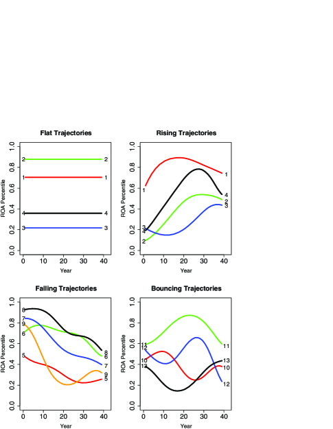
The behavior of individual firms was then characterized by using the MCMC history from the original analysis to get a maximum-likelihood estimate of the nonparametric alternative model. The almost-sure discreteness of the Dirichlet process means that this estimate is a mixture of a small number of flat and Gaussian-process trajectories. The 17 highest-weight trajectories in the MLE are in Figure 3; they are split into four loose categories reflecting different archetypes of company performance.
| GV | Company name | Flat 1 | Flat 2 | GP 7 | GP 8 | Other | Null |
|---|---|---|---|---|---|---|---|
| 11535 | Winn-Dixie Stores | 78 | 5 | 2 | |||
| 4828 | Delhaize America | 75 | 4 | 1 | |||
| 6830 | Lubrizol Corp | 64 | 4 | 1 | |||
| 7139 | Maytag Corp | 57 | 2 | 6 | |||
| 4323 | Emery Air Freight | 57 | 4 | 3 | |||
| 7734 | National Gas & Oil | 53 | 3 | 2 |
[]taGV refers to a unique corporate identifier.
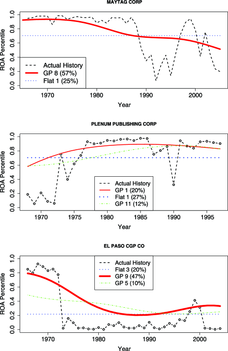
This allows an MLE clustering analysis: if in (14) is frozen at the mixture model in Figure 3 and the MCMC rerun, it is possible to flag companies that come from specific clusters. (Strictly speaking, only the first 17 atoms in the stick-breaking approximation of were frozen; others atoms were still considered, but they were allowed to vary.) Examples of the kinds of summaries available are in Table 2 and Figure 4.
Some general features of the methodology are apparent from these results:
-
•
There is substantial shrinkage of estimated mean trajectories back toward the global average (i.e., the 50th percentile). This is itself a form of multiplicity correction, in that extreme outcomes are quite likely to be attributed to chance even among those firms flagged as being from the alternative model.
-
•
Often there is no dominant trajectory in the MLE cluster set that characterizes a specific firm’s history. For the three firms in Figure 4, the probability is split among two or even three trajectories.
-
•
Model-averaged predictions of future performance are available with very little extra work, since full MCMC histories of each firm’s trajectory and residual model are available.
-
•
The MLE clustering analysis can provide evidence for historical evolution within specific firms, which is of great interest as the subject of follow-up case studies. Maytag, for example, displays markedly different performance patterns before and after 1987, which is reflected in its high probability of being from a falling trajectory (GP 8).
It must be emphasized that any such clustering analysis is at best an approximation, aside from the fact that the models themselves are also approximations. It relies, after all, upon a single point estimate of the trajectories composing the random distribution , and as such ignores uncertainty about the trajectories themselves. In the example at hand, several independent runs were conducted; each yielded a different MLE cluster set, but the same broad patterns (e.g., something like GP 8, something like Flat 3, and so on) emerged each time, suggesting at least some degree of robustness of the qualitative conclusions.
Still, the most reliable quantities are the inclusion probabilities computed from the full nonparametric analysis, which should form the basis of claims regarding which units are from the null and which are not.
6 Type-I error performance: a simulation study
This section recapitulates the simulation study of Section 2.4 using the more complicated models. The goal is to assess Type-I error performance by applying the methodology outlined here to a simulated data set where the number of nonzero trajectories is known.
The true residual model was constructed using a single MCMC draw from the stick-breaking representation of the nonparametric residual model for the corporate-performance data. This corresponded roughly to a 21-component mixture of AR(1) models (since 39 of the 60 atoms in the stick-breaking representation of had trivial weights), with many pairs that differed starkly in character.
To simulate the true mean trajectories, two independent sets of draws were taken from the prior in (11)–(13). In the first simulated set of trajectories, the true value of was fixed at in order to roughly approximate the fraction of discoveries on the ROA data. In the second set, was fixed at , to reflect a much sparser collection of signals. Upon sampling, these yielded and nonzero trajectories, respectively.
In both studies, each of these trajectories was convolved with a single independent vector of autoregressive noise drawn from the true —in other words, with a highly complex pattern of residual variation of the type that was shown to flummox the “single AR(1)” model of Section 2. For the sake of comparison, the same set of noise vectors was used for each experiment.
The results of these simulations were very encouraging for the Type-I error performance of the more complicated model. In the first simulated data set, of the nonzero trajectories were flagged as nonnulls with greater than probability. Only 24 of the 4374 null companies were falsely flagged, and of these, only had larger than a inclusion probability.
In the second simulated data set, of the known nonzero trajectories, had posterior inclusion probabilities greater than , and had inclusion probabilities greater than . Of the null trajectories, only had inclusion probabilities greater than (these two were only and ).
If is taken as the decision rule for a posteriori classification of a trajectory as nonnull (which again reflects a symmetric 0–1 loss function), then the realized false-discovery rates were only on 26 discoveries in the sparser case, and only on 321 discoveries in the denser case. (The closeness of these two realized false-discovery rates may simply be a coincidence of the particular values of chosen).
This suggests that a sizeable fraction of the firms flagged as nonnull trajectories in Section 5.2 represent nonaverage performers, and are not false positives.
7 Summary
This paper has described a framework for Bayesian multiple hypothesis testing in time-series analysis. The proposed methodology requires specifying only a few key hyperparameters for the nonparametric null and alternative models, and general guidelines for choosing these quantities have been given. Importantly, no ad-hoc “correction factors” are necessary in order to introduce a penalty for multiple testing. Rather, this penalty happens quite naturally by treating the prior inclusion probability as an unknown quantity with a noninformative prior.
Naïve characterizations of the null hypothesis are shown to have poor error performance, suggesting that the Bayesian procedure is highly sensitive to the accuracy of the null model used to describe an “average” time series. Yet once a sufficiently complex model for residual variation is specified, the procedure exhibits very strong control over the number of false-positive declarations, even in the face of firms with different autoregressive profiles. The difference between the results in Section 2.4 and Section 6 highlights the effectiveness and practicality of using nonparametric methods as a general error-robustification tactic in multiple-testing problems.
Posterior inference for a specific time series can be summarized in at least three ways: by quoting (the probability of that unit’s being from the alternative model), by performing an MLE clustering analysis as in Section 5.2, or by plotting the posterior draws of the unit’s nonzero mean trajectory. Plots such as Figure 4 can be quite useful for communicating inferences to nonexperts, as in the management-theory example considered throughout.
The companies flagged as impressive performers, of course, can only be judged so with respect to a particular notion of randomness: the DP mixture of autoregressive models described in Section 3. Inference on the nonzero trajectories can still reflect model misspecification, and cannot unambiguously identify companies that have found a source of sustained competitive advantage. This Dirichlet-process model, however, is a much more general statement of the null models postulated by Denrell (2003) and Denrell (2005), suggesting that the procedure described here can identify firms that, with high posterior probability, depart from randomness in a specific way that may be interesting to researchers in strategic management.
Supplement \stitleDPARtestingAoAS.zip \slink[doi]10.1214/09-AOAS252SUPP \slink[url]http://lib.stat.cmu.edu/aoas/252/supplement.zip \sdatatype.zip \sdescriptionThe data on corporate performance described in this paper is freely available for those with access to Standard and Poor’s Compustat database. Annual return on assets is computed as (net income)(total assets), which are Compustat codes NI and AT, respectively. ROA was further adjusted by regressing upon year, GICS industry codes, debt-to-equity ratio and sales, all of which are also available on Compustat. A simulated data set and the software necessary to implement these models are freely available in the supplemental file entitled “DPARtestingAoAS.zip.”
Acknowledgments
The author would like to thank Mumtaz Ahmed, Michael Raynor, Lige Shao, Jim Guszcza and Jim Wappler of Deloitte Consulting for their insight into the application discussed here, along with Andy Henderson of the University of Texas and Carlos Carvalho of the University of Chicago for all their helpful feedback.
References
- Antoniak (1974) Antoniak, C. (1974). Mixtures of Dirichlet processes with applications to Bayesian nonparametric problems. Ann. Statist. 2 1152–1174. \MR0365969
- Bartlett (1957) Bartlett, M. (1957). A comment on D.V. Lindley’s statistical paradox. Biometrika 44 533–534. \MR0086727
- Basu and Chib (2003) Basu, S. and Chib, S. (2003). Marginal likelihood and Bayes factors for Dirichlet process mixture models. J. Amer. Statist. Assoc. 98 224–235. \MR1965688
- Berger, Pericchi and Varshavsky (1998) Berger, J., Pericchi, L. and Varshavsky, J. (1998). Bayes factors and marginal distributions in invariant situations. Sankhya Ser. A 60 307–321. \MR1718789
- Berger and Guglielmi (2001) Berger, J. O. and Guglielmi, A. (2001). Bayesian and conditional frequentist testing of parametric model versus nonparametric alternatives. J. Amer. Statist. Assoc. 96 174–184. \MR1952730
- Berger and Pericchi (1996) Berger, J. O. and Pericchi, L. (1996). The intrinsic Bayes factor for model selection and prediction. J. Amer. Statist. Assoc. 91 109–122. \MR1394065
- Bigelow and Dunson (2005) Bigelow, J. and Dunson, D. (2005). Semiparametric classification in hierarchical functional data analysis. Technical report, Duke Univ., Dept. Statistical Science.
- Bowman and Helfat (2001) Bowman, E. H. and Helfat, C. E. (2001). Does corporate strategy matter? Strategic Management Journal 22 1–23.
- Carvalho and Scott (2009) Carvalho, C. M. and Scott, J. G. (2009). Objective Bayesian model selection in Gaussian graphical models. Biometrika 96 497–512.
- Cui and George (2008) Cui, W. and George, E. I. (2008). Empirical Bayes vs. fully Bayes variable selection. J. Statist. Plann. Inference 138 888–900. \MR2416869
- Dahl and Newton (2007) Dahl, D. B. and Newton, M. A. (2007). Multiple hypothesis testing by clustering treatment effects. J. Amer. Statist. Assoc. 102 517–526. \MR2325114
- Denrell (2003) Denrell, J. (2003). Vicarious learning, undersampling of failure, and the myths of management. Organizational Science 4 227–243.
- Denrell (2005) Denrell, J. (2005). Selection bias and the perils of benchmarking. Harvard Business Review April, 2005 114–119.
- Do, Muller and Tang (2005) Do, K.-A., Muller, P. and Tang, F. (2005). A Bayesian mixture model for differential gene expression. J. Roy. Statist. Soc. Ser. C 54 627–644. \MR2137258
- Dunson and Herring (2006) Dunson, D. and Herring, A. (2006). Semiparametric Bayesian latent trajectory models. Technical report, Duke Univ., Dept. Statistical Science.
- Escobar and West (1995) Escobar, M. and West, M. (1995). Bayesian density estimation and inference using mixtures. J. Amer. Statist. Assoc. 90 577–588. \MR1340510
- Ferguson (1973) Ferguson, T. (1973). A Bayesian analysis of some nonparametric problems. Ann. Statist. 1 209–230. \MR0350949
- Frühwirth-Schnatter and Kaufmann (2008) Frühwirth-Schnatter, S. and Kaufmann, S. (2008). Model-based clustering of multiple time series. J. Bus. Econom. Statist. 26 78–89. \MR2422063
- Gelfand, Kottas and MacEachern (2005) Gelfand, A., Kottas, A. and MacEachern, S. (2005). Bayesian nonparametric spatial modeling with Dirichlet process mixing. J. Amer. Statist. Assoc. 100 1021–1035. \MR2201028
- George and Foster (2000) George, E. I. and Foster, D. P. (2000). Calibration and empirical Bayes variable selection. Biometrika 87 731–747. \MR1813972
- Gramacy (2005) Gramacy, R. (2005). Bayesian treed Gaussian process models. Ph.D. thesis, Univ. California–Santa Cruz.
- Harrigan (1985) Harrigan, K. (1985). An application of clustering for strategic group analysis. Strategic Management Journal 6 55–73.
- Hawawini, Subramanian and Verdin (2003) Hawawini, G., Subramanian, V. and Verdin, P. (2003). Is performance driven by industry- or firm-specific factors? A new look at the evidence. Strategic Management Journal 24 1–16.
- Ishwaran and James (2001) Ishwaran, H. and James, L. (2001). Gibbs sampling methods for stick-breaking priors. J. Amer. Statist. Assoc. 96 161–173. \MR1952729
- Jefferys and Berger (1992) Jefferys, W. and Berger, J. (1992). Ockham’s razor and Bayesian analysis. Amer. Sci. 80 64–72.
- Jeffreys (1961) Jeffreys, H. (1961). Theory of Probability, 3rd ed. Oxford Univ. Press. \MR0187257
- Johnstone and Silverman (2004) Johnstone, I. M. and Silverman, B. W. (2004). Needles and Straw in Haystacks: Empirical-Bayes estimates of possibly sparse sequences. Ann. Statist. 32 1594–1649. \MR2089135
- Kleinman and Ibrahim (1998) Kleinman, K. and Ibrahim, J. (1998). A semiparametric Bayesian approach to the random effects model. Biometrics 54 921–938.
- Laud and Ibrahim (1995) Laud, P. and Ibrahim, J. (1995). Predictive model selection. J. Roy. Statist. Soc. Ser. B 57 247–262. \MR1325389
- Müller, West and MacEachern (1997) Müller, P., West, M. and MacEachern, S. (1997). Bayesian models for non-linear auto-regressions. J. Time Ser. Anal. 18 593–614. \MR1603392
- O’Hagan (1995) O’Hagan, A. (1995). Fractional Bayes factors for model comparison. J. Roy. Statist. Soc. Ser. B 57 99–138. \MR1325379
- Rasmussen and Williams (2006) Rasmussen, C. E. and Williams, C. (2006). Gaussian Processes for Machine Learning. MIT Press, Cambridge, MA. \MR2514435
- Ruefli and Wiggins (2000) Ruefli, T. W. and Wiggins, R. R. (2000). Longitudinal performance stratification: An iterative Kolmogorov–Smirnov approach. Management Sci. 46 685–692.
- Ruefli and Wiggins (2002) Ruefli, T. W. and Wiggins, R. R. (2002). Sustained competitive advantage: Temporal dynamics and the incidence and persistence of superior economic performance. Organization Science 13 81–105.
- Scott (2009) Scott, J. G. (2009). Supplement to “Nonparametric Bayesian multiple testing for longitudinal performance stratification.”
- Scott and Berger (2006) Scott, J. G. and Berger, J. O. (2006). An exploration of aspects of Bayesian multiple testing. J. Statist. Plann. Inference 136 2144–2162. \MR2235051
- Scott and Berger (2008) Scott, J. G. and Berger, J. O. (2008). Bayes and Empirical-Bayes multiplicity adjustment in the variable-selection problem. Discussion Paper 2008-10, Duke Univ., Dept. Statistical Science.
- Scott and Carvalho (2008) Scott, J. G. and Carvalho, C. M. (2008). Feature-inclusion stochastic search for Gaussian graphical models. J. Comput. Graph. Statist. 17 790–808.
- Wernerfelt (1984) Wernerfelt, B. (1984). The resource-based view of the firm. Strategic Management Journal 5 171–180.