Herschel-ATLAS: far-infrared properties of radio-selected galaxies*

Abstract

We use the Herschel-ATLAS science demonstration data to investigate the star-formation properties of radio-selected galaxies in the GAMA-9h field as a function of radio luminosity and redshift. Radio selection at the lowest radio luminosities, as expected, selects mostly starburst galaxies. At higher radio luminosities, where the population is dominated by AGN, we find that some individual objects are associated with high far-infrared luminosities. However, the far-infrared properties of the radio-loud population are statistically indistinguishable from those of a comparison population of radio-quiet galaxies matched in redshift and K-band absolute magnitude. There is thus no evidence that the host galaxies of these largely low-luminosity (Fanaroff-Riley class I), and presumably low-excitation, AGN, as a population, have particularly unusual star-formation histories. Models in which the AGN activity in higher-luminosity, high-excitation radio galaxies is triggered by major mergers would predict a luminosity-dependent effect that is not seen in our data (which only span a limited range in radio luminosity) but which may well be detectable with the full Herschel-ATLAS dataset.

* Herschel is an ESA space observatory with science instruments provided by European-led Principal Invstigator consortia and with important participation from NASA.

1 Introduction

It is well known that the increase in the star formation density of the Universe with redshift (e.g. Madau et al. 1996) is paralleled by an increase in the luminosity density of quasars (e.g. Boyle & Terlevich 1998), suggesting a link between galaxy assembly and accretion onto massive black holes. It is much less obvious whether this link is a direct one: is star-formation activity physically associated with AGN activity, and, if so, with what types of AGN activity is it associated? Although modelling suggests that the link may be a simple causal one, in the sense that mergers can trigger both AGN activity and star formation (e.g. Granato et al. 2004; di Matteo et al. 2005) this is a question that must be settled by direct observation of the AGN and star-formation properties of large samples of galaxies. Far-infrared observations, probing dust heated by young stars, provide one of the best methods of measuring the star-formation rate, but in the past it has been hard to obtain statistically robust samples, although this has improved recently (e.g. Serjeant & Hatziminaoglou 2009; Serjeant et al. 2010; Bonfield et al. 2010).

Radio-loud active galaxies are an important population in the study of the relationship between star formation and AGN activity. At the lowest radio luminosities (a population which is best studied at $z\sim 0$) the radio galaxy population is dominated by objects for which there is no evidence at any waveband for any radiatively efficient AGN activity, setting aside non-thermal emission associated with the nuclear jet (e.g. Hardcastle et al. 2009 and references therein). These objects have traditionally been called low-excitation radio galaxies (e.g. Hine & Longair 1979; Laing et al. 1994; Jackson & Rawlings 1997), but the differences between them and their ‘high-excitation’ counterparts are not only a matter of emission-line strength, but extend to optical (Chiaberge et al. 2002), X-ray (Hardcastle et al. 2006) and mid-IR (Ogle et al. 2006; Hardcastle et al. 2009). The low-excitation objects, where the AGN power output is primarily kinetic, clearly do not have the capability to regulate and eventually terminate star formation through coupling of their radiative output to cold gas. Instead the power of the AGN is put into the expansion of radio lobes, and therefore predominantly does work on the hot phase of the interstellar medium. At the highest radio luminosities, though, radio-loud AGN activity is almost always associated with radiatively efficient accretion, and these objects can have strong effects on both the hot and cold gas in their environments (cf. the ‘radio mode’/‘quasar mode’ dichotomy of Croton et al. 2006; powerful radio-loud AGN are operating in both modes simultaneously).

The relationship between radio-loud AGN and star formation might thus be expected to be a complex one, depending on radio luminosity, redshift and possibly radiative efficiency of the AGN, and indeed existing data present a picture of the relationship that seems to depend strongly on what AGN population (or individual object) is selected and which star-formation indicator is used. Hardcastle et al. (2007) argued that the nuclear differences between low- and high-excitation radio galaxies, suggesting a difference in accretion mode, might be explained by different sources of the accreting material, with the low-excitation sources powered by accretion (direct or otherwise) of the hot phase of the IGM, while high-excitation sources would be powered by cold gas supplied by mergers. This model is quantitatively viable in specific cases (Hardcastle et al. 2007; Balmaverde et al. 2008) and is qualitatively supported by the observation that low-excitation sources of similar radio powers prefer richer environments (Hardcastle 2004; Tasse et al. 2008). However, it also makes a prediction that high-excitation sources will be preferentially associated with gas-rich mergers and therefore star formation, which is borne out by observations both at low redshift (Baldi & Capetti 2008) and at $z\sim 0.5$ (Herbert et al. 2010).

Far-infrared/sub-mm studies of star formation in samples of radio galaxies have so far concentrated on high-redshift objects, in which emission at long observed wavelengths (e.g. 850 $\mu$m, 1.2 mm) corresponds to rest-frame wavelengths around the expected peak of thermal dust emission (e.g. Archibald et al. 2001; Reuland et al. 2004). Working at these high redshifts with the available flux-limited samples in the radio necessarily restricts these studies to the most powerful radio-loud AGN. However, the availability of observations at shorter far-IR wavelengths with the Herschel Space Observatory (Pilbratt et al. 2010) opens up the possibility of studies of very large populations of more nearby objects. In this paper, we present an analysis of all the radio-selected objects identified with galaxies detected by Herschel in the 14 deg² field acquired in the Science Demonstration Phase (SDP) of the Herschel Astrophysical Terahertz Large Area Survey (H-ATLAS: Eales et al. 2010). Although the full area of H-ATLAS (550 deg²) will be required to allow us to investigate the complete range of dependence of host galaxy properties on radio luminosity and redshift, we show that the new data shed some light on the nature of the hosts of the numerically dominant low-luminosity radio galaxy population.

Throughout the paper we use a concordance cosmology with $H_{0}=70$ km s^-1 Mpc^-1, $\Omega_{\rm m}=0.3$ and $\Omega_{\Lambda}=0.7$.

2 The data

The following images and catalogues were available to us:

1. PSF-convolved, background-subtracted images of the SDP field at the wavelengths of 250, 350 and 500 $\mu$m provided by the Spectral and Photometric Imaging Receiver (SPIRE) instrument on Herschel (Griffin et al. 2010). The construction of these images for the H-ATLAS SDP data is described in detail by Pascale et al. (2010) and Rigby et al. (2010). We do not consider the PACS (Photodetector Array Camera and Spectrometer; see Ibar et al. 2010) data here as they are not deep enough for detections of more than a small fraction of our targets. The SDP field consists of two observations over a 16 deg² region of the sky centred at $\rm{RA}=9^{\rm h}5^{\rm m}30^{\rm s}$, ${\rm Dec}=0^{\circ}5^{\prime}0^{\prime\prime}$. We restricted our analysis to the sub-region of the SDP field in which there was good data from both Herschel scans (hereafter the ‘good’ area of the SDP field); this covers 14.38 deg².

2. A catalogue of FIR sources detected in the SDP field, which includes any source detected at $5\sigma$ or better at any SPIRE wavelength (Rigby et al. 2010).

3. Radio source catalogues and images from the NRAO VLA Sky Survey (NVSS) (Condon et al. 1998) and Faint Images of the Radio Sky at Twenty-one centimetres (FIRST: Becker, White & Helfand 1995) surveys. These cover the whole of the SDP field.

4. Catalogues and images from the United Kingdom Infra-Red Telescope Deep Sky Survey – Large Area Survey (UKIDSS-LAS, hereafter LAS: Lawrence et al. 2007). The LAS covers only 92 per cent of the area of the SDP field.

5. Redshifts from the Galaxy And Mass Assembly survey (GAMA: Driver et al. 2009, 2010). GAMA is a deep spectroscopic survey with a limiting depths of $r_{\rm AB}<19.4$ mag, $z<18.2$ and $K_{\rm AB}<17.6$ in the SDP field; details of the target selection and priorities are given by Baldry et al. (2010) and Robotham et al. (2010). As described in more detail in Smith et al. (2010: hereafter S10), the GAMA catalogue for this area contains 12626 new spectroscopic redshifts in addition to 1673 redshifts from previous surveys in the area.

6. A catalogue of galaxies in the SDP field with photometric redshifts based on the LAS and Sloan Digital Sky Survey Data Release 7 (SDSS-DR7: Abazajian et al. 2009) photometric data, as described by S10. We filter this catalogue so as to require a K-band detection, to exclude any sources that are point-like in either the LAS or SDSS parent catalogues, and to impose the magnitude selection $r<22$ mag.

7. A list of identifications between these galaxies and detected sources in the H-ATLAS data, again as described by S10. For these identifications S10 define a reliability $R$ which is a measure of whether a single optical ($r$-band) source dominates the observed FIR emission; they suggest that only sources with $R>0.8$ be used for this to be the case. Throughout the paper we consider all sources in the S10 catalogue, but distinguish in our analysis between ‘reliable’ ($R>0.8$) and unreliable identifications.

8. A catalogue of optically selected quasars from the SDSS (Schneider et al. 2010) and 2dF-SDSS Luminous Red Galaxy and Quasar (2SLAQ: Croom et al. 2009) surveys in the SDP area, generated by Bonfield et al. (2010). We use this purely as a comparison population: the reader is referred to Bonfield et al. (2010) for details of the selection of these objects.

3 The radio-selected sample

We began by constructing a sample of radio-detected objects in the H-ATLAS SDP field. This was done in the following way:

1. We selected all catalogued NVSS sources in the ‘good’ area of the SDP field (796 in total). As the flux cutoff for the NVSS catalogue is $5\sigma$ (2.5 mJy), these are all clearly detected radio sources. The good short-baseline coverage of the NVSS data ensure that the NVSS flux densities are good estimates of the true total flux density of our targets.

2. We then cross-matched to the LAS K-band images by overlaying radio contours on LAS images, accepting only sources which had an association between the FIRST or, in a very few (5) cases, NVSS radio images and a K-band object with the appearance of a galaxy or a quasar. FIRST is used in preference to NVSS for identifications because of its much higher angular resolution, allowing less ambiguous identifications where compact radio components are present. This process excludes some weak or diffuse NVSS sources where FIRST detections were not available and where the NVSS position is inadequate to allow an identification with a LAS source. In addition, where NVSS sources were found to be blends of two or more FIRST sources, we corrected the NVSS flux density by scaling it by the ratio of the FIRST flux of the nearest source to the total FIRST flux. As mentioned above, the LAS covers only 92% of the area of the SDP field, so the choice to use this as our reference catalogue slightly reduces our coverage but does not affect the sample completeness in any way. We have 391 objects with LAS identifications.

3. Finally, we cross-correlated with the catalogue of galaxies with photometric redshifts (S10) on the basis of the LAS association. This gave us a total of 187 radio-loud sources in the SDP field. Where a spectroscopic redshift was available from the GAMA catalogue (including pre-existing SDSS redshifts) we used that in preference to a photometric redshift in subsequent analysis. 94 of our sources (50 per cent) had spectroscopic redshifts determined in this way. The median error on the photometric redshifts for all objects is 0.03 (see S10 for a discussion of the errors).

This process gives us a catalogue which is flux-limited in the radio (by virtue of the original selection from the NVSS) and also magnitude-limited in the optical (we require a K-band identification and also require $r<22$). In practice, this means that we have few sources with $z>0.7$ and none with $z>0.85$. The catalogue is also likely to be strongly biased against radio-loud quasars since we have excluded sources that appear point-like from our galaxy catalogue. This has the desirable effect that the measured luminosities will tend not to be strongly affected by beaming and that any contamination of the fluxes measured at Herschel wavelengths by non-thermal emission might be expected to be limited (cf. the results of Hes et al. 1995). Analysis of the full catalogue without the restriction of identification with (relatively) bright optical galaxies will be presented elsewhere (Virdee et al. in prep.): here we concentrate on the implications of the Herschel properties of these sources for the nature of radio-loud AGN activity.

Fig. 1 shows the radio luminosity-redshift plot for our radio-loud sample (here and throughout the paper we adopt $\alpha=0.8$, where $S\propto\nu^{-\alpha}$, for the $K$-correction in the radio luminosity calculations; $\alpha=0.8$ is a typical observed value for low-frequency selected objects, and we expect that the selection against point-like optical objects will tend to select against flat-spectrum radio sources). It will be seen that we probe a wide range of radio luminosities. At the low-luminosity, low-redshift end, we expect from existing analysis of the local 1.4-GHz luminosity function (e.g. Mauch & Sadler 2007) that the population will be dominated by luminous star-forming galaxies rather than radio-loud AGN, although a few AGN may still be present. The starburst luminosity function cuts off steeply above a few $\times 10^{23}$ W Hz^-1 at 1.4 GHz, so we expect that almost all objects above this luminosity will be radio-loud AGN, since we have no reason in the parent catalogue to be biased towards starburst galaxies. The Fanaroff-Riley break, i.e. the luminosity at which the population of radio galaxies switches from being dominated by objects of Fanaroff & Riley (1974)’s morphological class I to mostly containing objects of Fanaroff-Riley class II (hereafter these classes are abbreviated FRI and FRII) is at $1.2\times 10^{25}$ W Hz^-1 at 1.4 GHz, so our sample will be numerically dominated by FRIs, i.e. objects that are traditionally thought of as low-luminosity radio galaxies, but still has a significant number of objects at FRII luminosities. We have made no attempt to classify the objects morphologically in the radio using the NVSS or FIRST data, as these datasets tend to lack the surface-brightness sensitivity needed for reliable classification; morphological investigations will be discussed in a future paper.

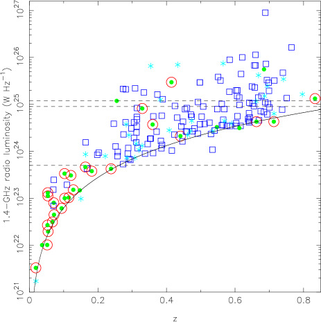
Figure 1: Radio luminosity of the radio-loud sample as a function of redshift. Sources nominally detected by Herschel (i.e. sources identified with Herschel objects in the S10 catalogue) are marked as filled green circles. If the association with the LAS galaxy is deemed ‘reliable’ in the S10 catalogue, the object is also marked with a red open circle. Any source not listed as detected in the catalogue, but detected down to the $2\sigma$ level in the 250-$\mu$m images, is shown as a light blue star. Non-detections are marked with blue open squares. The solid line corresponds to a nominal $5\sigma$ flux cutoff in the NVSS of 2.5 mJy. Sources lying significantly below this line do so as a result of the deblending process described in the text. Dashed horizontal lines show radio luminosities corresponding to (from bottom to top) the dividing line adopted in the text between starbursts and AGN; the expected luminosity for a maximal (4000 $M_{\odot}$ year^-1) starburst; and the luminosity corresponding to the Fanaroff-Riley break.

4 The far-IR properties of the sample

In this section we describe the properties of the sample in the far-IR. Throughout this section, FIR fluxes in the SPIRE bands are measured directly from the background-subtracted, PSF-convolved H-ATLAS SDP images described in Section 2, taking the flux density to be the value in the image at the pixel corresponding most closely to the LAS position of our targets, with errors estimated from the corresponding noise map. As discussed by Pascale et al. (2010), PSF-convolved maps provide the maximum-likelihood estimator for the flux density of an single isolated point source at a given position in the presence of thermal noise; this remains a reasonable approximation if there are small correlations between the positions of multiple sources, as we expect in real data due to physical clustering of objects. The flux densities we measure slightly underestimate the total flux density if the source is resolved, as we have verified by comparing our flux densities with those in the catalogue of Rigby et al. (2010), but this is only likely to be a problem at the lowest redshifts. We make an approximate correction for the mean background due to confusion by subtracting the mean flux level of the whole PSF-convolved map from each flux density measurement.

Throughout this section we distinguish between sources catalogued by Rigby et al. (2010) and lower-significance detections, down to the $2\sigma$ level, determined by the ratio of the flux density and the error measured by us from the maps at 250 $\mu$m: this distinction is only for the sake of illustration, in that it allows us to show the properties of sources weaker than those in the source catalogue, and the presence or absence of a $2\sigma$ detection forms no part of the quantitative analysis in the paper.

To convert between measured flux or luminosity densities at Herschel SPIRE wavelengths and total flux or luminosity in the far-IR band, as used in the literature, we have to adopt a model for the far-IR spectral energy distribution (SED), since in general we do not have enough data to fit models to each object. We investigated several possible SED templates, including an optically thick grey-body model whose parameters were determined from a fit to Arp 220 ($T=61.7$K, $\beta=1.54$, as used by Stevens et al. 2010), an optically thin grey body with parameters fitted to M82 ($T=44$ K, $\beta=1.55$) and the model fitted to normal galaxies in the SDP field (the S10 sample) by Dye et al. (2010) ($T=26$ K, $\beta=1.5$; cf. the very similar results, on a somewhat different sample of H-ATLAS sources, obtained by Amblard et al. 2010). These different choices of model parameters can make a significant difference (up to an order of magnitude) to the inferred total fluxes or luminosities, and also, via the $K$-correction, to their inferred dependence on redshift. Because of this, we chose to use the model adopted by Dye et al., which has the merit of being derived from a dataset that has considerable overlap with ours; for our current purposes the absolute normalization of the FIR luminosity is less important than the relative normalization, since our main conclusions will come from a comparison of the radio-loud objects with other samples. Detailed model fitting to the SEDs of radio-loud objects, and thus the possibility of considering such factors as evolution in temperature with luminosity or redshift will have to await a larger sample with a higher detection rate and will probably require additional constraints, such as the use of the PACS data; we plan to address this in a future paper. For the present work, we integrate the Dye et al. model between 8 and 1000 $\mu$m to obtain the total FIR fluxes and luminosities, for consistency with the approach used by other Herschel papers, bearing in mind that this integration almost certainly underestimates the total IR flux since it includes no component that radiates in the mid-IR.

4.1 Detections

As can be seen from Fig. 1, only 31 of the galaxies identified with our 187 sample objects have identifications with Herschel sources from the catalogue of S10; all but 6 of these are classed as ‘reliable’ identifications, as discussed in Section 2. The detection fraction is high at low radio luminosities (20/26 sources below $L_{1.4}=5\times 10^{23}$ W Hz^-1 are detected) but then drops off rapidly with increasing radio luminosity. Given the known behaviour of the starburst and AGN luminosity functions (Section 2) this is best explained in terms of a dominant starburst population at low radio luminosities in our radio-selected sample. To illustrate this, we have computed the parameter $q$, as originally defined by Helou et al. (1985), for each of the detected objects. $q=\log_{10}(S_{\rm IR}/(3.75\times 10^{12}\times S_{1.4})$, where $S_{\rm IR}$ is the integrated far-IR flux in W m^-2 and $S_{\rm 1.4}$ is in W Hz^-1 m^-2. We estimate $q$ from the 250-$\mu$m flux density using the grey-body model discussed above, taking proper account of $K$-correction. $q$ is plotted against radio luminosity in Fig. 2. For star-forming galaxies, $q$ by this definition is expected to have a typical value around 2.4 independent of radio luminosity, as found for example using Herschel data by Ivison et al. (2010) and Jarvis et al. (2010), as a result of the well-known radio-FIR correlation (e.g. Condon et al. 1991). We observe that most of the low-luminosity sources have $q$ values in the range 2–3. However, most of the detected high-luminosity sources have values of $q$ in the range 0-1.5, implying radio flux densities 1-2 orders of magnitude above the values expected from their FIR fluxes on the radio-FIR correlation, and the upper limits for non-detections are at a comparable level. We conclude that we are indeed seeing predominantly starbursts at $L_{1.4}<5\times 10^{23}$ W Hz^-1 but that above this we are predominantly detecting genuine radio-loud AGN. These results are unaltered if we use values of $q$ determined from fits to the 70-500 $\mu$m SEDs of the detected Herschel sources (Jarvis et al. 2010) and the values of $q$ obtained are also consistent with that more detailed analysis. In what follows we use $L_{1.4}<5\times 10^{23}$ W Hz^-1 as an approximate luminosity cutoff to exclude the bulk of objects with $q$ values consistent with being standard starbursts. While we recognise that more luminous starbursts than this can and do exist, the small number of objects observed to have $L_{1.4}>5\times 10^{23}$ W Hz^-1 and $q>2$ suggests that few are present in our sample.

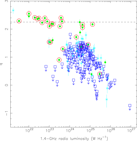
Figure 2: The parameter $q$ (as defined in the text) as a function of radio luminosity for the sample. $q$ is estimated from the flux in the 250-$\mu$m maps in all cases as described in the text. Colours and symbols are as for Fig. 1. The dashed horizontal line gives the median $q$ (2.25) for the 20 reliably detected sources with $L_{1.4}<5\times 10^{23}$ W Hz^-1. A $2\sigma$ upper limit on $q$ is plotted for undetected sources.

4.2 Stacking analysis

Table 1: Mean bin flux densities and K-S probabilities that the Herschel fluxes of objects in redshift bins are drawn from the background distribution, as a function of wavelength. Low probabilities (below 1 per cent) imply significant differences between the bin being considered and the distribution of flux densities measured from randomly selected positions in the sky, as described in the text.

Catalogued	$z$ range	Objects	Mean bin flux density (mJy)			K-S probability (%)
sources?		in bin	250 $\mu$m	350 $\mu$m	500 $\mu$m	250 $\mu$m	350 $\mu$m	500 $\mu$m
Included	0.00 – 0.10	15	$396.1\pm 1.7$	$160.6\pm 1.9$	$58.8\pm 2.3$	$<10^{-3}$	$<10^{-3}$	$<10^{-3}$
	0.10 – 0.20	14	$125.1\pm 1.7$	$52.2\pm 1.9$	$18.0\pm 2.4$	$<10^{-3}$	0.004	0.7
	0.20 – 0.35	39	$13.3\pm 1.0$	$7.2\pm 1.2$	$2.7\pm 1.4$	2.4	2.6	20.7
	0.35 – 0.50	40	$6.9\pm 1.0$	$5.6\pm 1.1$	$2.2\pm 1.4$	0.07	2.3	40.1
	0.50 – 0.65	43	$5.9\pm 1.0$	$4.7\pm 1.1$	$3.6\pm 1.4$	1.0	1.3	1.9
	0.65 – 0.85	36	$10.0\pm 1.1$	$5.5\pm 1.2$	$4.3\pm 1.5$	0.007	3.9	5.2
Excluded	0.00 – 0.10	4	$133.7\pm 3.3$	$69.2\pm 3.6$	$26.3\pm 4.5$	30.6	49.1	92.9
	0.10 – 0.20	6	$5.3\pm 2.6$	$6.0\pm 3.0$	$1.9\pm 3.7$	14.9	25.7	33.1
	0.20 – 0.35	36	$3.1\pm 1.1$	$3.6\pm 1.2$	$1.9\pm 1.5$	14.9	18.8	30.5
	0.35 – 0.50	37	$4.1\pm 1.1$	$4.1\pm 1.2$	$2.0\pm 1.5$	0.5	4.5	59.0
	0.50 – 0.65	41	$3.6\pm 1.0$	$3.0\pm 1.1$	$2.9\pm 1.4$	2.3	2.7	4.0
	0.65 – 0.85	32	$5.3\pm 1.1$	$2.1\pm 1.3$	$3.2\pm 1.6$	0.05	19.0	9.0

Table 2: Mean bin flux densities and K-S probabilities that the Herschel fluxes of objects in luminosity bins are drawn from the background distribution, as a function of wavelength. Notes as for Table 1.

Catalogued	Range in	Objects	Mean bin flux density (mJy)			K-S probability (%)
sources?	$\log_{10}(L_{1.4})$	in bin	250 $\mu$m	350 $\mu$m	500 $\mu$m	250 $\mu$m	350 $\mu$m	500 $\mu$m
Included	21.0 – 23.7	27	$290.6\pm 1.2$	$118.0\pm 1.4$	$42.2\pm 1.7$	$<10^{-3}$	$<10^{-3}$	$<10^{-3}$
	23.7 – 24.3	32	$2.4\pm 1.1$	$0.5\pm 1.3$	$-1.3\pm 1.6$	28.3	69.8	12.5
	24.3 – 24.6	35	$11.5\pm 1.1$	$10.7\pm 1.2$	$5.6\pm 1.5$	0.010	0.05	1.1
	24.6 – 25.0	40	$9.2\pm 1.0$	$4.5\pm 1.1$	$2.3\pm 1.4$	0.8	10.3	48.4
	25.0 – 25.6	38	$7.1\pm 1.1$	$4.7\pm 1.2$	$4.0\pm 1.5$	0.9	12.2	5.1
	25.6 – 27.3	15	$9.1\pm 1.7$	$7.2\pm 1.9$	$6.8\pm 2.3$	0.10	0.4	1.2
Excluded	21.0 – 23.7	7	$79.2\pm 2.5$	$42.7\pm 2.8$	$15.1\pm 3.4$	15.2	39.2	99.5
	23.7 – 24.3	32	$2.4\pm 1.1$	$0.5\pm 1.3$	$-1.3\pm 1.6$	28.3	69.8	12.5
	24.3 – 24.6	31	$6.6\pm 1.2$	$7.6\pm 1.3$	$4.7\pm 1.6$	0.07	0.3	10.8
	24.6 – 25.0	37	$2.5\pm 1.1$	$1.8\pm 1.2$	$2.0\pm 1.5$	5.0	16.1	42.9
	25.0 – 25.6	35	$3.2\pm 1.1$	$2.4\pm 1.2$	$3.0\pm 1.5$	3.2	32.6	14.1
	25.6 – 27.3	14	$7.7\pm 1.7$	$5.9\pm 1.9$	$6.6\pm 2.4$	0.3	0.8	1.8

Table 3: Mean bin flux densities of the comparison galaxy population and K-S probabilities that the Herschel fluxes of objects in redshift bins are drawn from this galaxy population, as a function of wavelength.

$z$ range	Radio-loud	Mean galaxy flux density (mJy)			K-S probability (%)			Comparison
	objects in bin	250 $\mu$m	350 $\mu$m	500 $\mu$m	250 $\mu$m	350 $\mu$m	500 $\mu$m	galaxies
0.00 – 0.10	15	$22.3\pm 0.2$	$11.0\pm 0.3$	$4.7\pm 0.3$	$<10^{-3}$	$<10^{-3}$	$<10^{-3}$	770
0.10 – 0.20	14	$15.5\pm 0.1$	$7.4\pm 0.1$	$3.0\pm 0.2$	1.4	2.0	4.6	2913
0.20 – 0.35	39	$12.6\pm 0.1$	$6.4\pm 0.1$	$2.9\pm 0.1$	7.3	4.7	6.5	5481
0.35 – 0.50	40	$7.9\pm 0.1$	$4.5\pm 0.1$	$2.0\pm 0.1$	92.5	65.6	98.7	14660
0.50 – 0.65	43	$6.9\pm 0.1$	$4.4\pm 0.1$	$2.2\pm 0.1$	41.9	97.5	35.1	11905
0.65 – 0.85	36	$9.5\pm 0.1$	$6.5\pm 0.1$	$3.1\pm 0.2$	90.6	58.7	80.9	2971

Since the vast majority of our radio sources are undetected at the $5\sigma$ limit of the H-ATLAS source catalogue (Rigby et al. 2010), we need to use statistical methods to calculate the properties of the source population. We elected to stack the sample in bins corresponding to redshift and radio luminosity to investigate the way in which the far-IR properties varied with those two parameters.

To establish quantitatively whether sources in the bins were significantly detected, we measured flux densities from 100,000 randomly chosen positions in the field; a Kolmogorov-Smirnov (K-S) test could then be used to see whether the sources from our sample were consistent with being drawn from a population defined by the random positions. Using a K-S test rather than simply considering the calculated uncertainties on the measured fluxes allows us to account for the non-Gaussian nature of the noise as a result of confusion. We chose the boundaries of our luminosity bins in such a way that the lowest-luminosity bin contained all sources with $L<5\times 10^{23}$ W Hz^-1 and we also placed a bin boundary at the nominal Fanaroff-Riley transition luminosity, while otherwise trying to keep roughly similar numbers of sources per bin. Results are given in Tables 1 and 2, which also show the mean flux density at each wavelength for every bin. We see that the sources in the lowest luminosity bin and the lowest two redshift bins are very strongly distinguished from the random background population, as expected from Fig. 1; sources at intermediate radio luminosity or redshift are not distinguished from the background, but then several higher-luminosity or higher-$z$ bins are distinguished from the background at significance levels ranging from 2 to $>3\sigma$, at least at 250 $\mu$m. As expected (since the beam is larger and the potential for confusion greater), the significance drops off with increasing wavelength. Importantly, these results still hold, though obviously with somewhat reduced significance, if we exclude the formally detected sources (those with identifications in the catalogue) from the analysis, as shown in the bottom halves of Tables 1 and 2. Setting aside the lowest-luminosity and lowest-redshift bins ($z<0.2$, $L_{1.4}<5\times 10^{23}$ W Hz^-1), where the exclusion of detections removes almost all the sources, all the bins that are significantly detected with the inclusion of the formally detected sources are still detected at 95 per cent confidence or better on the K-S test at 250 $\mu$m if those sources are excluded, and many bins are more significantly detected than that; so at least at high radio luminosities or redshifts we are not simply seeing the effect of a very few far-IR-bright objects. We emphasise, though, that it is the K-S statistics that include the detected objects (left-hand side of these tables) that determine whether a given bin is actually detected.

We were also able to compare with the properties of galaxies that were not identified with radio sources. To do this we selected all objects identified as galaxies in the photometric redshift catalogue of S10 that had a LAS detection and a determined spectroscopic (GAMA) or photometric redshift, imposing the cutoff $z<0.85$, but were not identified with radio sources and that lay on the ‘good’ SDP field area so that photometry in the Herschel bands was possible. This gave 59,817 galaxies in total. The population of radio-selected sources is significantly ($>99.5$ per cent confidence) different from this general galaxy population as a whole on a K-S test at all SPIRE wavebands. However, if we break both populations down by redshift, using the same binning scheme as previously and imposing the additional requirement that the comparison galaxies lie in the same K-band absolute magnitude range as the radio-loud hosts (which restricts us to 38,700 galaxies), we see that this effect is completely dominated by the sources with $z<0.2$, i.e. the sources that we identify as star-forming galaxies (Table 3). The higher-redshift objects, which we expect to be radio-loud AGN, are indistinguishable, statistically, in their FIR flux distribution from galaxies selected in a similar way but without radio counterparts, and their mean flux densities at each wavelength are also very similar. These similarities are understandable, since we know that, at least at the low radio luminosities we are considering, radio galaxy hosts very often have the appearance of passively evolving ellipticals with no evidence either for strong star formation or for an obscured, radiatively efficient AGN, and the K-band selection and magnitude cutoff of our comparison population will have the effect of including many similar objects. We return to this point below.

4.3 Far-IR luminosity and star formation

We estimated far-IR luminosities in our bins using a modified version of the method of Serjeant & Hatziminaoglou (2009). The value of this approach is that it aims to account for the intrinsic scatter in the flux density of objects in bins as well as the scatter due to (thermal and confusion) noise when the luminosities are averaged; the reader is referred to Serjeant & Hatziminaoglou (2009) for a detailed description of the method. For each redshift or luminosity bin, we characterised the intrinsic scatter in the measured flux densities using a maximum-likelihood fit. Serjeant & Hatziminaoglou fitted a Gaussian to the flux density distribution of each bin, but as Gaussian fits were rather poor to some of our bins, we elected to use a lognormal distribution in flux density (which also has the merit of being constrained to positive flux density values), applying a prior that is uniform in log space to the mean. Rather than assuming an underlying Gaussian distribution of the noise, we used the actual noise distribution in the data (as determined from our random flux measurements) and used Monte-Carlo simulation to derive the probability distribution of flux densities (which, after the addition of noise, can be negative) and thus the model likelihood for any given set of parameters. This allowed us to determine the best-fitting values for the intrinsic distribution in flux densities using a Markov-Chain Monte Carlo (MCMC) algorithm (see Mullin & Hardcastle 2009 for a description of the code). Having done this, we took noise-weighted means of the luminosities in each bin in the manner described by Serjeant & Hatziminaoglou (2009), for simplicity at this stage making the approximation that both the intrinsic scatter in the distribution and the noise were Gaussian so that they could be added in quadrature to determine the weights. (We note that the overall result of this procedure is reassuringly similar to what we obtain if we simply take the mean of the luminosities using only the measured noise values; the results are not dominated by the weights derived from the intrinsic scatter estimates.) As in Section 4.1, the luminosities were calculated from the measured 250-$\mu$m fluxes (since the detections of stacks are most significant in this band, as discussed in Section 4.2) on the assumption of a grey-body template SED.

Results are plotted in Fig. 3. Looking first at the results of binning by radio luminosity (top-hand panel) we see that, as expected, the lowest-luminosity radio bin has a reasonably high mean FIR luminosity around $10^{11}L_{\odot}$. The highest FIR luminosities of objects in this bin are comparable to those of starbursts like Arp 220, which suggests a comparably high star-formation rate. The second bin has a much lower luminosity (which, given that this bin is not detected in our K-S test analysis, should be considered to be an upper limit) corresponding to star formation rates $\la 5M_{\odot}$ year^-1. This is the effect of moving from a selection criterion that selects mostly starbursts to one that selects mostly AGN, and it immediately shows that the lowest-luminosity radio-loud AGN tend to have little or no star formation. The remaining radio bins have FIR luminosities somewhat higher than the mean in the first bin, and show at most a weak positive trend with radio luminosity; these luminosities would correspond (using the starburst relation from Kennicutt (1998), and bearing in mind the many caveats associated with doing so) to total star formation rates between 50 and 100 $M_{\odot}$ year^-1, which might be associated either with the host galaxy of the radio source itself (in which case these would be high star formation rates for quiescent ellipticals) or with nearby galaxies in a host group or cluster. It is important to bear in mind that the star-formation rates we quote here, and the values plotted in Fig. 3, will be affected by systematic uncertainties in the correction from 250-$\mu$m rest-frame flux to total mid-IR luminosity, as discussed at the start of this Section. The relative star-formation rates should be robust, but the absolute normalizations might be systematically wrong by a significant factor. We note, however, that the star-formation rates we derive are quite consistent with those derived by Seymour et al. (2010) in a study of radio-loud objects in the Herschel Multi-Tiered Extragalactic Survey (HerMES).

The results of luminosity stacking must be interpreted in the light of the stacking in redshift bins (Fig. 3, lower panel). Here we perform an identical stacking analysis using the normal galaxy population, selected as defined in the previous Section, as a control. As we expected given the results of the K-S tests, we see that the FIR luminosities of radio-selected objects are much higher than those of comparably selected galaxies in the lowest two redshift bins, corresponding to the objects likely to be starburst galaxies. However, above this redshift, we see very close agreement between the radio-loud objects and the general galaxy population. The difference between the two even at the highest redshifts (and therefore highest radio luminosities) is little more than $1\sigma$ with the current data.

Finally, we can also compare with the properties of optically selected quasars from the Bonfield et al. (2010) sample in the same redshift bins. There are only 67 unique quasars in this sample in the $z<0.85$ redshift range, so the sample size is considerably smaller than for our radio-selected objects; there are also no objects with $z<0.10$. However, the individual redshift bins are all significantly detected at 99 per cent confidence or better on K-S tests, so we can validly use these small samples to compare with the radio galaxies. None of the quasars in this redshift range is identified with a radio source in our sample. We see (Fig. 3, lower panel) that there is a clear trend for the luminosities of these quasars to lie significantly above the luminosities of both the normal galaxies and the radio-selected objects, though this tendency appears weaker at higher redshift.

5 Discussion and conclusions

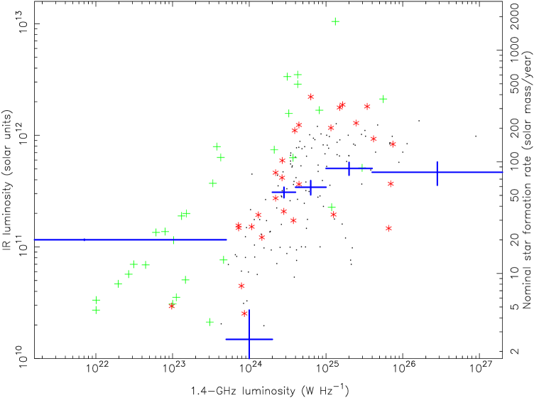
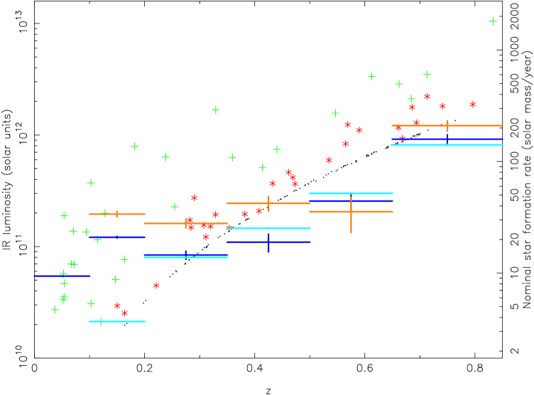
Figure 3: Far-IR luminosity, derived from the measured 250-$\mu$m luminosity, as a function of (top) 1.4-GHz luminosity and (bottom) redshift for the radio-loud sample, showing both individual objects and the results of stacking as described in the text. Green crosses show identifications in the catalogue of S10; red stars show individual objects down to $2\sigma$, and black dots show $2\sigma$ upper limits. Error bars on individual luminosities are not plotted for clarity. Blue solid lines in both panels are the results of stacking and show the mean luminosity and associated error bars in each of the radio luminosity or redshift bins defined in the text. Cyan solid lines in the lower panel show the results of a similar stacking analysis applied to the comparison sample of normal galaxies described in the text, and orange solid lines show the results of stacking the quasar sample also described in the text. The right-hand axis shows the conversion between far-IR luminosity and star-formation rate, assuming a Kennicutt (1998) starburst relationship; the locus of the limits in the bottom figure thus shows the limiting star-formation rate to which we are sensitive for individual objects.

The most obvious conclusion to be drawn from Section 4.3 is that the FIR properties of radio galaxies and those of a comparably-selected population of radio-quiet objects are very similar, given the data that are presently available to us. The selection of our comparison sample could clearly be improved with more data; for example, our radio non-detections at high redshift will clearly include some lower-luminosity radio-loud objects, while we have not attempted to use the available optical data to select exclusively elliptical galaxies. But taking the observations at face value, we see no evidence that radio galaxy hosts behave any differently in the FIR from a matched population of radio-quiet galaxies. We do not believe that the incompleteness of our optical identifications of the NVSS/FIRST sources should affect this conclusion: the missing objects are likely either quasars (and therefore undesirable because of the possibility of contamination by non-thermal emission) or higher-redshift objects (see below).

Should we be surprised by our result? We begin by noting that we do not expect any effect from any radiatively efficient AGN in these radio galaxies — the typical mid-IR luminosities (at around 15 $\mu$m) of radio-loud AGN of comparable radio luminosity to the most powerful objects in our sample are 1-2 orders of magnitude lower than what we observe in the present sample, if they are detected at all (Hardcastle et al. 2009) and the emission from the torus of radio galaxies believed to be hosting an obscured AGN would be expected, and is observed, to peak in the mid-IR (e.g. Haas et al 2004). We also do not expect to see any synchrotron contamination in the FIR, bearing in mind that the typical flux density of our sources at 1.4 GHz is a few mJy while the flux density at 250 $\mu$m (1.2 THz) of detected sources is an order of magnitude higher, and that, as discussed above, our selection criteria should strongly favour steep-spectrum objects. We are thus safe to interpret the FIR luminosities as telling us about star formation, subject to the usual caveats about young stars being the dominant source of dust heating in these objects (Kennicutt 1998).

The picture appears then to be that the host galaxies of these low-luminosity radio-loud AGN have, on average, no more – or less – star formation than the general population selected to have similar K-band magnitudes. This is the first time it has been possible to investigate this with a large sample in the FIR at these low radio luminosities; earlier work studying high-$z$ radio galaxies and radio-loud quasars with SCUBA (e.g. Archibald et al.2001; Willott et al. 2002; Rawlings et al. 2004) probed radio luminosities which were almost all significantly larger than those studied here (for example, all the sources in Archibald et al. have $L_{1.4}>4\times 10^{28}$ W Hz^-1), while studies of low-$z$ radio galaxies have generally used shorter wavelengths, such as the 60 $\mu$m of IRAS (e.g. Yates & Longair 1989; Hes et al. 1995) or the 70 $\mu$m of Spitzer (e.g. Dicken et al. 2009) where the general consensus seems to be that AGN-related thermal and non-thermal emission dominates the measured flux densities. Our results will therefore be useful for updating the latest models of far-infrared emission emanating from AGN and their hosts (e.g. Wilman et al. 2010).

The result above is certainly consistent with our general picture of the properties of radio-loud AGN and their hosts. We know that at $z=0$ the vast majority of low-luminosity radio galaxies are hosted by quiescent ellipticals (e.g., Lilly & Longair 1984; Best et al. 2005); in these low-power objects there is in general little evidence for major, gas-rich mergers and so we would expect to see little or no ongoing star formation (cf. Kaufmann, Heckman & Best 2008). But it is interesting to ask how this can be reconciled with the fact that there does seem to be a strong association between AGN activity and star formation when the AGN are selected at other wavebands (e.g. Serjeant et al. 2010). The answer is probably related to the two populations of radio-loud AGN, low-excitation and high-excitation radio galaxies, described in Section 1. The radio luminosity functions of low-excitation and high-excitation radio galaxies clearly have different slopes, since low-excitation objects are strongly numerically dominant at low radio luminosities but almost completely absent at the highest luminosities: the transition in terms of numerical dominance seems to take place at radio luminosities comparable to, but probably slightly above, the conventional Fanaroff-Riley break. Our radio-loud sample is thus numerically completely dominated by objects that are likely to be low-excitation radio galaxies, which we would expect, based on the models discussed in Section 1, to have little or no association with star formation. Only in the highest radio-luminosity bin might we expect to see substantial numbers of high-excitation radio galaxies with evidence for star formation, and the statistics there are poor. It should be noted that Fig. 3 clearly shows that there are individual objects with both high radio luminosities and high inferred star formation rates at all radio luminosities above a few $\times 10^{24}$ W Hz^-1; these may well be high-excitation radio galaxies associated with gas-rich mergers, and they certainly account for the relatively high mean FIR luminosities and star-formation rates in the high-radio-luminosity bins in that Figure. The idea that high-excitation AGN, if present, would be associated with higher star-formation rates is borne out, at least qualitatively, by the position of the quasars from the sample of Bonfield et al. (2010) in the lower panel of Fig. 3, though we caution that we have necessarily made no attempt to match these in host galaxy properties to the radio-selected or normal galaxies.

With deeper optical/IR data, better spectroscopy and radio data from our GMRT observations, plus broader coverage with Herschel (all of which will be available in the near future), we can test this qualitative picture in a number of ways. With more objects of higher radio luminosity, we will be able to break the luminosity-redshift degeneracy inherent to the present sample (the results presented here give no new information on whether the far-IR luminosity of radio galaxy hosts depends principally on redshift or on radio luminosity, a problem first identified by Rawlings et al. 2004). The SDP data represent only 1/40th of the 570 deg² of the full H-ATLAS data, so our eventual sample size will increase by a large factor: in particular, we expect $\sim 6$ FRIIs per square degree (Wilman et al. 2008) up to the highest redshift so the full H-ATLAS will give us $>3000$ powerful sources. In addition, even with the current data we have optical/IR identifications for less than half of the original radio sample (Section 3) so in principle many high-redshift radio sources are already there and just await identification; the availability of VIKING data (1.4 mag deeper than UKIDSS-LAS) will allow us to identify powerful radio sources out to $z\sim 2.5$ (Jarvis et al. 2001; Willott et al. 2003) and so we will be able both to extend the stacking study and, probably, to increase the number of Herschel-detected sources, allowing a study of the detected population as a function of radio luminosity and morphology. Secondly, the model outlined above implies that we would expect any excess FIR luminosity in radio galaxies to be associated not only with indicators of star formation at other wavelengths (e.g. optical galaxy colours) but also with indicators of high-excitation AGN activity such as strong narrow emission lines (which can be investigated with GAMA and other spectroscopy), a mid-IR excess (which might be visible in survey data from the Wide-field Infrared Survey Explorer, WISE) and obscured nuclear X-ray emission (many H-ATLAS fields have available X-ray data). With the larger sample and the wider availability of multi-wavelength diagnostics provided by the full H-ATLAS project, it should be possible to carry out a definitive test of this model.

References

- [] Abazajian, K.N., et al. 2009, ApJS, 182, 543
- [] Amblard, A., et al. 2010, A&A, 518, L9
- [] Archibald, E.N., Dunlop, J.S., Hughes, D.H., Rawlings, S., Eales, S.A., Ivison, R.J., 2001, MNRAS, 323, 417
- [] Baldry, I.K., et al. 2010, MNRAS, 404, 86
- [] Balmaverde, B., Baldi, R.D., Capetti, A., 2008, A&A, 486, 119
- [] Best, P.N., Kauffmann, G., Heckman, T.M., Brinchmann, J., Charlot, S., Ivezić, Z., White, S.D.M., 2005, MNRAS, 362, 25
- [] Boyle, B.J., Terlevich, R.J., 1998, MNRAS, 293, L49
- [] Chiaberge, M., Macchetto, F.D., Sparks, W.B., Capetti, A., Allen, M.G., Martel, A.R., 2002, ApJ, 571, 247
- [] Condon, J.J., Anderson, M.L., Helou, G., 1991, ApJ, 376, 95
- [] Condon, J.J., Cotton, W.D., Greisen, E.W., Yin, Q.F., Perley, R.A., Taylor, G.B., Broderick, J.J., 1998, AJ, 115, 1693
- [] Croom, S., et al. 2009, MNRAS, 392, 19
- [] Croton, D., et al., 2006, MNRAS, 365, 111
- [] di Matteo T., Springel, V., Hernquist, L., 2005, Nat, 433, 604
- [] Dicken, D., et al., 2009, ApJ, 694, 268
- [] Driver, S.P., et al. 2009, A&G 50 5.12
- [] Driver, S.P., et al. 2010, MNRAS submitted
- [] Dye, S., et al. 2010, A&A in press, arXiv:1005.2411
- [] Eales, S., et al. 2010, PASP, 122, 499
- [] Fanaroff, B.L., Riley, J.M., 1974, MNRAS, 167, 31P
- [] Granato, G.L., De Zotti, G., Silva, L., Bressan, A., Danese, L., 2004, ApJ, 600, 580
- [] Griffin, M.J., et al. 2010, A&A in press, arXiv:1005.5123
- [] Haas, M., et al., 2004, A&A, 424, 531
- [] Hardcastle, M.J., 2004, A&A, 414, 927
- [] Hardcastle, M.J., Evans, D.A., Croston, J.H., 2006, MNRAS, 370, 1893
- [] Hardcastle, M.J., Evans, D.A., Croston, J.H., 2007, MNRAS, 376, 1849
- [] Hardcastle, M.J., Evans, D.A., Croston, J.H., 2009, MNRAS, 396, 1929
- [] Helou, G., Soifer, B.T., Rowan-Robinson, M., 1985, ApJ, 298, L7
- [] Herbert, P.D., Jarvis, M.J., Willott, C.J., McLure, R.J., Mitchell, E., Rawlings, S., Hill, G.J., Dunlop, J.S., 2010, MNRAS in press
- [] Hes, R., Barthel, P.D., Hoekstra, H., 1995, A&A, 303, 8
- [] Hine, R.G., Longair, M.S., 1979, MNRAS, 188, 111
- [] Ivison, R., et al 2010, A&A in press (arXiv:1005.1072)
- [] Jackson, N., Rawlings, S., 1997, MNRAS, 286, 241
- [] Jarvis, M.J., Rawlings, S., Eales, S., Blundell, K.M., Bunker, A.J., Croft, S., McLure, R.J., Willott, C.J., 2001, MNRAS, 326, 1585
- [] Jarvis, M.J., et al. 2010, MNRAS submitted
- [] Kauffmann, G., Heckman, T.M., Best, P.N., 2008, MNRAS, 384, 953
- [] Laing, R.A., Jenkins, C.R., Wall, J.V., Unger, S.W., 1994, in Bicknell G.V., Dopita M.A., Quinn P.J., eds, The First Stromlo Symposium: the Physics of Active Galaxies, ASP Conference Series vol. 54, San Francisco, p. 201
- [] Lilly, S.J., Longair, M.S., 1984, MNRAS, 211, 833
- [] Madau, P., Ferguson, H.C., Dickinson, M.E., Giavalisco, M., Steidel, C.C., Fruchter, A., 1996, MNRAS, 283, 1388
- [] Mauch, T., Sadler, E., 2007, MNRAS, 375, 931
- [] Mullin, L.M., Hardcastle, M.J., 2009, MNRAS, 398, 1989
- [] Ogle, P., Whysong, D., Antonucci, R., 2006, ApJ, 647, 161
- [] Pilbratt, G.L., et al., 2010, A&A in press (arXiv:1005.5331)
- [] Rawlings, S., Willott, C.J., Hill, G.J., Archibald, E.N., Dunlop, J.S., Hughes, D.H., 2004, MNRAS, 351, 676
- [] Robotham, A…, et al. 2010, PASA, 27, 76
- [] Schneider, D.P., et al 2010, AJ, 139, 2360
- [] Serjeant, S., Hatziminaoglou, E., 2009, MNRAS, 397, 265
- [] Serjeant, S., et al. 2010, A&A in press (arXiv:1005.2410)
- [] Smith, D.J.B., et al 2010, MNRAS submitted [S10]
- [] Tasse, C., Best, P.N., Röttgering, H., Le Borgne, D., 2008, A&A, 490, 893
- [] Willott, C.J., Rawlings, S., Archibald, E.N., Dunlop, J.S., 2002, MNRAS, 331, 435
- [] Willott, C.J., Rawlings, S., Jarvis, M.J., Blundell, K., 2003, MNRAS, 339, 173
- [] Wilman, R.J., et al., 2008, MNRAS, 388, 1335
- [] Yates, M.G., Longair, M.S., 1989, MNRAS, 241, 29