Resonant $\gamma\to a$ transition in magnetar magnitosphere

Abstract

The effect of a magnetized plasma on the resonant photoproduction of axions on the electromagnetic multipole components of the medium, $i\to f+a$, has been considered. It has been shown that the axion resonant emissivity, due to various reactions involving particles of the medium, is naturally expressed in terms of the emissivity of the photon $\to$ axion transition. The number of axions produced by the equilibrium cosmic microwave background radiation in the magnetar magnetosphere has been calculated. It has been shown that the resonant mechanism under consideration is inefficient for the production of cold dark mass.

1 Introduction

The axion proposed by Peccei and Quinn [1] to solve the problem of the conservation of the CP invariance of strong interactions remains not only the most attractive solution to the CP problem, but also is the most probable candidate for cold dark matter in the Universe. Since the Peccei-Quinn symmetry violation scale $f_{a}$ is large, the interaction of axions with matter is very weak (the coupling constant is $f_{a}^{-1}\lesssim 10^{-8}$  GeV^-1 [2]). In view of this circumstance, the experimental detection of the axion is a complicated problem.

At the same time, the effect of an active medium on reactions involving axions can both catalyze these reactions and additionally (as compared to $f_{a}^{-1}$) suppress them, depending on the parameters of the medium (temperature $T$, chemical potential $\mu$, and magnetic field $B$). It is of particular interest to analyze the processes involving axions in an extremely strong magnetic field $B\gg B_{e}$ ($B_{e}=m^{2}/e\simeq 4.41\times 10^{13}$ G is the critical magnetic field).  Such conditions can exist in the magnetospheres of magnetars, a specific class of neutron stars with magnetic fields that are much stronger than $B_{e}$ and reach $10^{14}-10^{16}$ G [3, 4, 5]. Moreover, a multicomponent (electron-positron or ion) plasma can exist near such objects. In particular, electron number density in the region of closed field lines is estimated as [6]

$$n\sim\left(\frac{1}{R_{NS}\Omega}\right)n_{GJ}\simeq 5\cdot 10^{5}\,\left(\frac{10\,\mbox{rad/s}}{\Omega}\right)\left(\frac{10\,\mbox{km}}{R_{NS}}\right)n_{GJ}\gg n_{GJ},$$ (1)

where

$$n_{GJ}=7\cdot 10^{-2}\frac{B}{P}\,\mbox{cm}^{-3}\simeq 3\cdot 10^{13}\,\mbox{cm}^{-3}\left(\frac{B}{100B_{e}}\right)\left(\frac{10\,\mbox{s}}{P}\right)$$ (2)

is the Goldreich-Julian charge number density [7].

Nowadays, there exists a growing interest to investigation of effective axion production processes in astrophysical object with such extremal conditions. In recently paper [8] was considered the conversion of axions to photons in strong magnetic fields of neutron stars (Primakoff effect). It was shown, that the photon $\to$ axion resonant conversion is absented for density plasma in magnetar environment and allowable axion mass $10^{-6}\lesssim m_{a}\lesssim 10^{-2}$ eV. But then, the scattering processes of photons on the plasma components in the magnetar magnetosphere with axion emission become important.

Therefore, it is of interest to consider the production of axions in the general reaction $i\to f+a$ (see the diagram in Fig. 1) under conditions very strong magnetic field and relatively dense plasma ($n\gg n_{GJ}$), where the initial $(i)$ and final $(f)$ states can involve the electromagnetic multipole components of the medium. The closed circle in Fig. 1 is the effective $g_{\gamma a}$ interaction vertex (diagrams in Fig. 2). It is easy to see that the process under consideration can be resonant owing to the presence of a virtual photon. Such process was considered recently in [9] and our investigation bases on results of this paper. A similar situation for the region close to resonance was recently considered also in [10] for the Compton scattering of relic photons on the electrons and positrons of the magnetar magnetosphere. However, we will show below that the results obtained in [10] are inaccurate.

Figure 1: Feynman diagram for the general process $i\to f+a$. Double lines mean that the effect of the external field on the initial and final states is exactly taken into account.

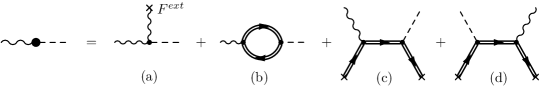
Figure 2: Feynman diagrams for the effective $\gamma a$ interaction vertex.

2 Amplitude of process $i\to f+a$

In the existing axion models the process $i\to f+a$ in the presence of the external magnetic field can be described by the effective Lagrangian [2]

$${\cal L}_{a\gamma}(x) = g_{a\gamma}\widetilde{F}^{\mu\nu}[\partial_{\nu}A_{\mu}(x)]a(x)+\frac{g_{af}}{2m_{f}}[\bar{\psi}_{f}(x)\gamma^{\mu}\gamma_{5}\psi_{f}(x)]\partial_{\mu}a(x)-$$

$$- Q_{f}[\bar{\psi}_{f}(x)\gamma^{\mu}\psi_{f}(x)]A_{\mu}(x).$$

Here $A_{\mu}$ is the four-potential of the quantized electromagnetic field, $\widetilde{F}^{\mu\nu}$ is the dual tensor of the external field, $\psi_{f}(x)$ and $a(x)$ are the quantized fermion and axion fields, respectively, $g_{a\gamma}=\alpha\xi/2\pi f_{a}$, where $\xi$ is the model dependent parameter about unit, $g_{af}=C_{f}m_{f}/f_{a}$ is the dimensionless Yukawa axion-fermion coupling constant with the model dependent factor $C_{f}$, $Q_{f}$ is the electric charge of the fermion (for the electron $Q_{f}=-e$).

Using Lagrangian (2), the $i\to f+a$ amplitude can be represented in the form

$${\cal M}^{a}_{i\to f}=-\frac{{\cal M}^{\gamma}_{if}{\cal M}_{\gamma\to a}}{q^{\prime 2}-{\cal P}^{(\varepsilon)}(q^{\prime})}\,,$$ (4)

where ${\cal M}^{\gamma}_{if}$ is the amplitude of the process $i\to f+\gamma$ with the emission of a photon in the final state;

$${\cal M}_{\gamma\to a}=i\bar{g}_{a\gamma}(\varepsilon\widetilde{F}q^{\prime})$$ (5)

is the photon $\to$ axion transition amplitude; $q^{\prime\mu}=(\omega^{\prime},{\bf k}^{\prime})$ is the axion four-momentum; and ${\cal P}^{(\varepsilon)}(q^{\prime})$ is the eigenvalue of the photon polarization operator, which corresponds to the polarization vector $\varepsilon_{\alpha}$. The effective axion-photon coupling constant $\bar{g}_{a\gamma}$ can be represented as the sum of three terms $\bar{g}_{a\gamma}=g_{a\gamma}+\Delta g^{B}_{a\gamma}+\Delta g^{pl}_{a\gamma}$. The first term corresponds to the interaction of the axion with the electromagnetic field caused by the Adler anomaly (the diagram in Fig. 2a), the second term describes the axion-photon interaction through an electron loop (the diagram in Fig. 2b), and the third term corresponds to forward scattering on the electrons and positrons of the plasma (the diagrams in Figs. 2c and 2d). A similar calculation of $\Delta g^{B}_{a\gamma}$ and $\Delta g^{pl}_{a\gamma}$ was previously performed in [11] and [12], respectively. Here, we only note that to correctly calculate $\Delta g^{B}_{a\gamma}$, the subtraction corresponding to the Adler anomaly should be made in it [11]. In particular, this fact was disregarded in [10], which is one of the causes of why the results obtained in that work are incorrect.

Further, we represent ${\cal P}^{(\varepsilon)}(q^{\prime})$ in the form ${\cal P}^{(\varepsilon)}=\Re-i\Im$, where $\Re=Re({\cal P})$ and $\Im=Im({\cal P})$ are the real and imaginary parts of the polarization operator, respectively. The latter is due to the processes of the absorption and emission of photons in the plasma and, according to [13], is expressed as

$$\Im=\omega^{\prime}\left(e^{\omega^{\prime}/T}-1\right)\Gamma_{cr},$$ (6)

in terms of the total photon production width

$$\Gamma_{cr}=\sum_{i,f}\int|{\cal M}^{\gamma}_{if}|^{2}d\Phi_{if},$$ (7)

where $d\Phi_{if}$ is the phase volume element of the states $i$ and $f$ for the process $i\to f+\gamma$ taking into account the corresponding distribution functions, and summation is performed over all of the possible initial and final states.

3 Axion emissivity

Taking into account the above consideration, the axion emissivity (the loss of energy from a unit volume per unit time due to the axion escape), due to the reactions involving the particles of the plasma, can be represented in the form

$$Q=\sum_{i,f}\int d\Phi_{if}\,d\Phi^{\prime}\,\omega^{\prime}|{\cal M}^{a}_{i\to f}|^{2}\,,$$ (8)

$d\Phi^{\prime}=\frac{d^{3}k^{\prime}}{(2\pi)^{3}2\omega^{\prime}}$ is the phase volume element of the axion. Taking into account Eqs. (4) and (6), $Q$ is represented in the form

$$Q=\int\frac{d\Phi^{\prime}\,|{\cal M}_{\gamma\to a}|^{2}}{e^{\omega^{\prime}/T}-1}\,\frac{\Im}{(q^{\prime 2}-\Re)^{2}+\Im^{2}}\,.$$ (9)

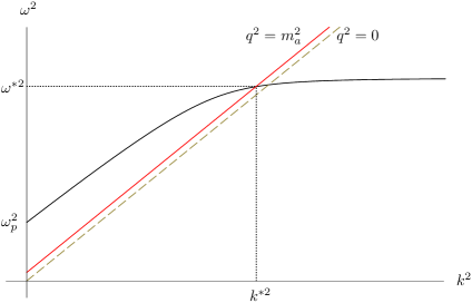
Figure 3: Photon (black curve) and axion (red line) dispersion law. The crosspoint of the photon and axion dispersion curves corresponds to resonant point.

According to Eq. (9), the most significant contribution to the axion luminosity comes from the resonance region, i.e., from the vicinity of the intersection point of the dispersion curves of the axion, $q^{\,\prime 2}=m_{a}^{2}$, and photon, $q^{\,\prime 2}=\Re$, so that the photon becomes real (Fig. 3). Near the resonance, the part of the integrand in Eq. (9) can be interpolated by the $\delta$ function

$$\frac{\Im}{(q^{\prime 2}-\Re)^{2}+\Im^{2}}\simeq\pi\,\delta(q^{\prime 2}-\Re)\,.$$ (10)

Using the properties of the $\delta$ function, we can represent Eq. (9) in the form

$$\frac{\Im}{(q^{\prime 2}-\Re)^{2}+\Im^{2}}\simeq\pi\,\int\frac{d^{3}k}{2\omega}Z_{\varepsilon}\delta^{4}(q-q^{\prime})\,,$$ (11)

where $Z_{\varepsilon}^{-1}=1-\frac{\partial\Re}{\partial\omega^{2}}$ corresponds to the renormalization of the photon wavefunction, $q^{\mu}=(\omega,{\bf k})$ is the photon four-momentum.

Taking into account Eq. (11), emissivity (9) can be written as

$$Q\simeq(2\pi)^{4}\,\int\frac{d^{3}k}{2\omega(2\pi)^{3}}\,\frac{\omega}{e^{\omega/T}-1}\int\frac{d^{3}k^{\prime}}{2\omega^{\prime}(2\pi)^{3}}\,Z_{\varepsilon}|{\cal M}_{\gamma\to a}|^{2}\delta^{4}(q-q^{\prime})\,.$$ (12)

This expression exactly corresponds to the formula for the axion emissivity in the $\gamma\to a$ process. Thus, the axion emissivity in the resonance region, owing to the reactions involving the particles of the medium, is naturally expressed in terms of the photon $\to$ axion transition emissivity.

After integration with $\delta$ functions, emissivity is reduced to the form

$$Q=\frac{\bar{g}_{a\gamma}^{2}(eB)^{2}}{32\pi^{2}\alpha}\,\int_{-1}^{1}\frac{dx}{e^{\omega/T}-1}\,\frac{Z_{\varepsilon}k(\varepsilon\widetilde{\varphi}q)^{2}}{\left|1-\frac{d\omega^{2}}{dk^{2}}\right|}\bigg{|}_{k=k^{*}}\,.$$ (13)

Here $x=\cos{\theta}$, where $\theta$ is the angle between the photon momentum and the magnetic field, $k^{*}=k^{*}(\theta)$ is a root of the equation $\omega^{2}(\vec{k})=m_{a}^{2}+k^{2}$, $\widetilde{\varphi}_{\alpha\beta}=\widetilde{F}_{\alpha\beta}/B$.

The further calculation of the emissivity significantly depends on the plasma characteristics finally determining the dispersion properties of photons. We consider below two particular cases.

i) Weakly magnetized dense plasma, $m_{a}^{2}\ll eB\ll T^{2},\mu^{2}$. In this case, $\varepsilon_{\alpha}$ is the polarization vector of the longitudinal plasmon

$$\varepsilon_{\alpha}=\sqrt{\frac{q^{2}}{(uq)^{2}-q^{2}}}\,\left(u_{\alpha}-\frac{(uq)}{q^{2}}\,q_{\alpha}\right),$$ (14)

where $u_{\alpha}$ is the four velocity of the plasma. Emissivity (13) has the simple form

$$Q=\frac{\bar{g}_{a\gamma}^{2}(eB)^{2}}{48\pi^{2}\alpha}\,\frac{(k^{*})^{3}}{e^{k^{*}/T}-1}\,$$ (15)

in complete agreement with the results reported in [14]. Note that $k^{*}$ in this case is independent of $\theta$ and is determined only by the plasma parameters.

ii) Strongly magnetized plasma, $eB\gg m^{2},\,\mu^{2}\gg T^{2}$. Here $\varepsilon_{\alpha}=(q\widetilde{\varphi})_{\alpha}/\sqrt{(q\widetilde{\varphi}\widetilde{\varphi}q)}$, $\Re\simeq(q\widetilde{\varphi}\widetilde{\varphi}q)\left(\frac{\omega_{p}^{2}(1+\eta)}{\omega^{2}}-\eta\right)$, $\eta=(\alpha/3\pi)(B/B_{e})$ and plasma frequency $\omega_{p}$ is related to the electron density as $\omega^{2}_{p}=4\pi\alpha n/m$. Moreover, in the strong magnetic field limit the contributions of diagrams b, c and d in Fig. 2 in the effective axion-photon coupling constant are suppressed by field, so that $\bar{g}_{a\gamma}\simeq g_{a\gamma}$.

However, in contrast to the case of weakly magnetized plasma, the final analytical expression for emissivity can be obtained only in some particular cases.

• When the axion mass is the smallest parameter of the problem, i.e., $\omega_{p},\,T\gg m_{a}$ (e.g., the production of light axions (axion mass smaller than $10^{-5}$ eV) in the magnetar magnetosphere (see Eq. (1)), $k^{*}\simeq\omega_{p}\sqrt{1+1/\eta}$ and emissivity can be represented in the form

  $$Q\simeq\frac{g_{a\gamma}^{2}(eB)^{2}}{16\pi^{2}\alpha}\,\omega_{p}^{3}\frac{(1+\eta)^{3/2}}{\eta^{5/2}}\left(\exp{\left[\frac{\omega_{p}}{T}\sqrt{1+\frac{1}{\eta}}\,\right]}-1\right)^{-1}\,.$$ (16)

• When $\omega_{p}\gg T\sim m_{a}$, the integral in Eq. (13) is accumulated in the region $x\simeq 1$ and, hence, $k^{*}\simeq\omega_{p}$. In this case, emissivity is suppressed exponentially by plasma density

  $$Q \simeq \frac{g_{a\gamma}^{2}(eB)^{2}}{16\pi^{2}\alpha}\,Tm_{a}^{2}\,e^{-\omega_{p}/T}\,.$$ (17)

In addition to emissivity, it is also of interest to estimate the number of axions produced in the magnetar magnetosphere in unit volume per unit time through the above resonant mechanism, because the axion is one of the main candidates for the constituents of cold dark matter. Similar to Eqs. (13), (16), and (17), we obtain

$$\frac{dN}{dtdV}=\frac{g_{a\gamma}^{2}(eB)^{2}}{32\pi^{2}\alpha}\,\int_{-1}^{1}\frac{dx}{e^{\omega/T}-1}\,\frac{kZ_{\varepsilon}(\varepsilon\widetilde{\varphi}q)^{2}}{\omega\left|1-\frac{d\omega^{2}}{dk^{2}}\right|}\bigg{|}_{k=k^{*}}\,,$$ (18)

$$\frac{dN}{dtdV}\simeq\frac{g_{a\gamma}^{2}(eB)^{2}}{16\pi^{2}\alpha}\,\omega_{p}^{2}\frac{1+\eta}{\eta^{2}}\times\left(\exp{\left[\frac{\omega_{p}}{T}\sqrt{1+\frac{1}{\eta}}\,\right]}-1\right)^{-1}\,,\quad\omega_{p},\,T\gg m_{a},$$ (19)

$$\frac{dN}{dtdV} \simeq \frac{g_{a\gamma}^{2}(eB)^{2}}{16\pi^{2}\alpha}\,\frac{Tm_{a}^{2}}{\omega_{p}}\,e^{-\omega_{p}/T}\,,\quad\omega_{p}\gg T\sim m_{a}.$$ (20)

In particular, for the number of axions produced by the cosmic microwave background radiation ($T\sim m_{a}\sim 10^{-3}$ eV), the minimum plasma density ($\sim 10^{15}$ cm^-3) at which the resonant mechanism is allowed $(\omega_{p}\gtrsim m_{a})$, and the magnetic field $B=100B_{e}$, Eq. (18) gives the estimate $dN/(dVdt)\sim 10^{10}$ axions in cm^-3 per second. Thus, $10^{29}$ axions are produced per second in the volume of the magnetar magnetosphere ($\sim 10^{19}$ cm³) with the strong magnetic field. In the most optimistic variant, estimating the number of magnetars in the Galaxy as $\sim 10^{6}$, we conclude that they produce $\sim 10^{51}$ axions in $\sim 10^{9}$ yr; therefore, the density of axions in the Galaxy should be $n_{a}\sim 10^{-21}$ cm^-3, which is much lower than the density of baryons $n_{b}\sim 10^{-7}$ cm^-3 $\gg n_{a}$.

Consequently, the statement made in [10] that ”vicinities of magnetic neutron stars with fields $B\gg B_{e}$ can be high power generators conversing the cosmic microwave background radiation to the axion component of the cold dark mass” is invalid.

4 Conclusion

We have considered the resonant photoproduction of axions in the general reaction $i\to f+a$. It has been shown that the calculation of axion emissivity owing to this process is reduced to the calculation of the emissivity of the photon $\to$ axion transition. Two particular cases of weakly and strongly magnetized plasmas have been analyzed. The number of axions produced by the equilibrium cosmic microwave background radiation in the magnetar magnetosphere has been estimated. It has been shown that this mechanism is inefficient for the production of cold dark mass even at the plasma density $n\sim 10^{15}$ cm ^-3.

Acknowledgements

We express our deep gratitude to the organizers of the Seminar “Quarks-2010” for warm hospitality.

This work was performed in the framework of realization of the Federal Target Program “Scientific and Pedagogic Personnel of the Innovation Russia” for 2009 - 2013 (project no. NK-410P-69) and was supported in part by the Ministry of Education and Science of the Russian Federation under the Program “Development of the Scientific Potential of the Higher Education” (project no. 2.1.1/510).

References

- [1] R. D. Peccei, H. R. Quinn, Phys. Rev. Lett. 38, 1440 (1977); Phys. Rev. D 16, 1791 (1977).
- [2] G. G. Raffelt Stars as Laboratories for Fundamental Physics. Chicago: University of Chicago Press, 1996. 664 p.
- [3] R. C. Duncan, C. Thompson, Astrophys. J. 392, L9 (1992).
- [4] C. Thompson, R. C. Duncan, Mon. Not. R. Astron. Soc. 275, 255 (1995).
- [5] R. C. Duncan, C. Thompson, Astrophys. J. 473, 322 (1996).
- [6] C. Thompson, M. Lyutikov, S. R. Kulkarni, Astrophys. J. 574, 332 (2002).
- [7] P. Goldreich, W. H. Julian, Astrophys. J. 157, 869 (1969).
- [8] M. S. Pshirkov, S. B. Popov Zh. Eksp. Teor. Fiz. 135, 440 (2009) [JETP, 108, 384, (2009)].
- [9] N. V. Mikheev, D. A. Rumyantsev, Yu. E. Shkol’nikova, Pis’ma v Zh. Eksp. Teor. Fiz. 90, 668 (2009) [JETP Letters, 90, 604, (2009)].
- [10] V. V. Skobelev, Zh. Eksp. Teor. Fiz. 132, 1121 (2007) [JETP 105, 982 (2007)].
- [11] L. A. Vassilevskaya, N. V. Mikheev, and O. S. Ovchinnikov, Yad. Fiz. 62, 1662 (1999) [Phys. At. Nucl. 62, 1556 (1999)].
- [12] N. V. Mikheev, E. N. Narynskaya, Mod. Phys. Lett. A 21, 433 (2006).
- [13] H. A. Weldon, Phys. Rev. D28, 2007 (1983).
- [14] N. V. Mikheev, G. Raffelt, L. A. Vassilevskaya, Phys. Rev. D58, 055008.