Self-organized criticality in a network of
economic agents with finite consumption

Abstract

We introduce a minimal agent model to explain the emergence of heavy-tailed return distributions as a result of self-organized criticality. The model assumes that agents trade their economic outputs with each other composing a complex network of agents and connections. Further, the incoming degree of an agent is proportional to the demand on its goods, while its outgoing degree is proportional to the supply. The model considers a collection of economic agents which are attracted to establish connections among them to make exchange at a price form by supply and demand. With our model we are able to reproduce the evolution of the return of macroscopic quantities (indices) and to correctly retrieve the non-trivial exponent value characterizing the amplitude of drops in several indices in financial markets, relating it to the underlying topology of connections. The distribution of drops in empirical data is obtained by counting the number of successive time-steps for which a decrease in the index value is observed. All eight financial indexes show an exponent $m\sim 5/2$. Finally, we present mean-field calculations of the critical exponents, and of the scaling relation $m=\tfrac{3}{2}\gamma-1$ between the exponent $m$ for the distribution of drops and the topological exponent $\gamma$ for the degree distribution.

1 Introduction: Observing SOC in financial data

The application of statistical physics to finance and economy was boosted in the last decades, particularly with the analysis of financial data in 1973 by Black, Scholes and Merton[1], explaining the price evolution in an organized market. More recently[5, 6], such application found important developments with the introduction of procedures for quantitatively describing financial data, by explicitly deriving a Fokker-Planck equation for the empirical probability distributions which catches the typical non-Gaussian heavy tails of financial time-series, across scales. However, as Mandelbrot pointed out[7], other typical features are observed in the variation of prices, namely scale invariance behavior[8], which cannot be explained by means of a cascade model. The modeling of financial index dynamics and other complex phenomena taking into account non-Gaussianity and scale invariant behavior has been indicated as an appealing problem to address in the scope of finance analysis and statistical physics[8, 9], particularly in what concerns the emergence of Self-organized Criticality (SOC)[10] in financial markets.

SOC is typically observed in slowly-driven non-equilibrium systems with extended degrees of freedom and a high level of nonlinearity. Many individual examples have been identified since the Bak, Tang and Wiesenfeld (BTW) model in the pioneer paper in Ref. [10], describing the occurrence the emergence of power-laws in different systems. This simple model shows avalanches of arbitrary sizes in one cellular automaton mimicking a sand pile, where at each sand cell is toppled to other cells when a certain threshold level is reached. The toppling may trigger subsequent topplings composing what one can interpret as an avalanche.

Surprisingly, such cascade of topplings was reported to be observed in other contexts, assuming the proper interpretation, and even when not completely accepted, SOC become established as a strong candidate for explaining the phenomenology of such systems. For example, evolution of species seems to lay around a self-organized critical state of periods with almost no mutations and then periods with arbitrarily large sequences of mutations exhibiting a power-law distribution[11]. Another important example is earthquake statistics, which was already known to obey Gutenberg-Richter law[12], a power-law which agrees with SOC phenomenology. The fluctuations in economic systems, described for instances by financial markets indices or prices were also reported by Mandelbrot[7], Mantegna and Stanley[8] and other to show scale invariance behavior. But to the best of our knowledge there is still no clear connection between the power-laws seen in financial markets and SOC.

Using an agent model to characterize two groups of traders, Lux and Marchesi presented some evidence that scaling in finance emerges as a result of the interactions between individual market agents[13]. Agent-based models of financial markets have been intensively studied. For a review see Ref. [14] and references therein. It has been claimed that agent models are able to complement the approach borrowed from social sciences, where from one theory a specific model is derived and applied to empirical data[15]. An agent model is typically constructed by starting to identify the statistical features in the data of interest and then to implement the necessary ingredients in our model in order to generate data with the same features.

In this paper, we aim to show that two fundamental assumptions in Economics are sufficient for the emergence of a self-organized critical state in the social environments where humans trade, an environment that we call henceforth the financial system and that we map into a set of interconnected agents. Further, we will show that the under such assumptions, the model is also able to reproduce the scaling features observed in empirical data.

The first assumption is that humans are attracted to each other to exchange labor due to biological specialization that made the species more efficient when each specimen could perform the tasks to which is more capable[16]. The second is that the amount of labor exchanged by each of the two involved agents in an economic relation is ruled by the law of supply and demand[16]. Based on these principles, which are straightforwardly translated to the physical context, we will show that the assumption for the system to be in equilibrium cannot be sustained, differently from the Brownian particle approach. Since labor must be produced in order that agents can establish labor exchanges, on each agent there is an “energy” dissipation that must finite. Inserted in a system where agents are impelled to create more economic exchanges then, physically, this configuration corresponds to a self-organized critical system[10]. In other words, the self-organized critical state emerges due to finite “energy” consumption in economic agents. Though the term energy used in the economical context is not the same as physical energy, since it does not necessarily satisfy the thermodynamic constraints, we will use the term in the economical context only. For example, human labor is assumed as “energy” delivered by the agent to a neighbor, which rewards the agent with an energy that the agent accumulates. The balance between the labor produced for the neighbors and the reward received from them may be positive (agent profits) or negative (agent accumulates debt). For simplicity, we omit henceforth the quotation marks.

Since the main concern in risk management deals with the distribution of the so-called drops in financial market indices, we restrict ourselves to that side of the distribution. In a financial market index, one drop is defined as the decrease of the index from one time-step to the next one. Each drop on financial markets results from the economical crash of one or more agents, being represented by the collapse of those agents. Such local crashes appear at no particular moment and may cascade into an avalanche of arbitrary size, i.e. a succession of an arbitrary large number of local economical crashes, taken as a global economical crisis.

We start in section 2 by introducing the minimal model that translates the two fundamental assumptions described above into a two body problem without additional assumptions. In the section 3, we frame the two body problem in the many body problem assuming that agents connect each other by preferential attachment[17] as expected from other human networks to show the critical behavior of the system with a typical exponent around $5/2$, characterizing the critical behavior in the system, and that the return distribution probability depends directly on the topology of the network. We show that our model reproduces the typical behavior of financial indices drops, in particular showing that empirical indices have similar exponent values, around $5/2$. The exponent $5/2$ is derived quantitatively based in branching processes and mean-field assumptions and show that it depends linearly on the underlying complex network exponent. In section 4 we draw the conclusions.

2 Minimal Model for Economic Relations

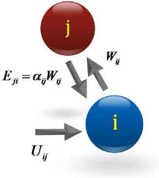
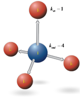
Figure 1: Left: Illustration of an economical connection between two agents $i$ and $j$. Agent $i$ transfer labor $W_{ij}$ to agent $j$ receiving an energy $E_{ij}=\alpha_{ij}W_{ij}$ where $\alpha_{ij}$ measures how well the labor is rewarded: agent $i$ has an outgoing connection (production) and agent $j$ an incoming connection (consumption). This interaction attributes to agent $i$ an amount of “internal energy” $U_{ij}=W_{ij}-E_{ij}$ that can be summed up over all agents connections up to a threshold $U_{th}$ beyond which it is distributed among the neighbors (see text). Right: The transfer of labor is done according to a preferential attachment scheme: the agent prefers to work for agents which have already a large number of labor connections to them.

In this section we introduce an agent-model that considers a collection of $N$ agents operating as energy transducers into the economic space in the form of labor. Agents, labeled $i$ and $j$ in Fig. 1 (left), establish among them bi-directed connections characterized as follows. When agent $i$ delivers labor $W_{ij}$ to agent $j$ it receives in return a proportional amount of agent $j$ labor, $E_{ij}=\alpha_{ij}W_{ij}$. Both quantities $E_{ij}$ and $W_{ij}$ can be regarded as forms of energy, in the economic space. Henceforth we consider all interchange of energy in units of $W_{ij}=1$.

The factor $\alpha_{ij}$ is a (dimensionless) measure of the labor price, defined as

$$\alpha_{ij}=\frac{2}{1+e^{-(k_{out,i}-k_{in,j})}}$$ (1)

where $k_{out,i}$ and $k_{in,j}$ are the number of outgoing connections of agent $i$ and the number incoming connections of agent $j$, respectively (see Fig. 1). A large (small) $k_{in,j}$ indicates a large (small) supply for agent $i$ and a large (small) $k_{out,i}$ indicates a large (small) demand of agent $i$.

When $\alpha_{ij}=1$, agent $j$ returns to agent $i$ the same amount of labor it receives from agent $i$. This happens when $k_{in,j}=k_{out,i}$, yielding $W_{ij}=E_{ij}$, i.e. when there is local balance between supply and demand. This value $\alpha_{ij}=1$ is the middle value between the asymptotic limits $k_{in,j}\gg k_{out,i}$ ($\alpha_{ij}\sim 0$) and $k_{in,j}\ll k_{out,i}$ ($\alpha_{ij}\sim 2$) which satisfy basic economic principles[16]. Namely, in the limit $k_{in,j}\gg k_{out,i}$, the labor of agent $j$ is in much greater demand than the labor of $i$, and thus agent $j$ is in a position to pay $i$ very little in return. In other words, for $\alpha_{ij}<1$ the labor of agent $i$ is paid by $j$ below the amount of energy $W_{ij}$ it delivers, i.e. agent $i$ loses from the connection (trade) and loses a certain amount of energy, $U_{ij}=W_{ij}-E_{ij}>0$. For $\alpha_{ij}>1$ the opposite occurs, i.e.  when $k_{in,j}<k_{out,i}$, agent $i$ has more supply of labor than agent $j$ has demands for its labor. In the limit $k_{in,j}\ll k_{out,i}$, the value of $\alpha_{ij}$ could in principle be any finite value larger than one. To guarantee an equal range length for both the situation when agent $i$ profits from agent $j$ and the situation when agent $i$ looses from agent $j$, we consider the range $\alpha_{ij}\in[0,2]$, which implies the limit $\alpha_{ij}=2$ for $k_{in,j}\ll k_{out,i}$ as can be seen from Eq. (1).

The energy balance for each trade, $W_{ij}-E_{ij}$, translates into an energy balance for each node that takes into account all outgoing and incoming connections the agent has: $U_{i}=\sum_{j\in{\cal V}_{out,i}}(W_{ij}-E_{ij})+\sum_{j\in{\cal V}_{in,i}}(E_{ji}-W_{ji})$ where ${\cal V}_{out,i}$ and ${\cal V}_{in,i}$ are the outgoing and incoming vicinity of agent $i$, with $k_{out,i}$ and $k_{in,i}$ neighbors respectively.

We also assume that each agent $i$ chooses its neighbors according to a preferential attachment scheme, following the Barabási-Albert-Jeong method[17]. This scheme is as follows: one starts with a small amount of agents totally interconnected, and adds iteratively one agent with one connection to one of the previous agents, chosen from a probability function proportional to their number of connections. Thus, agents having a large amount of connections are more likely to be chosen for a new connection than other agents.

Here, this topology underlies the empirical observation in economic-like systems that agents are more likely to deliver their work to agents receiving already significantly amount of work. See Ref. [17] for several examples such as the Internet and the airport network among other. See Fig. 1.

Since we drop the assumption of an equilibrium system, these particles we call agents can experiment the boundaries of the system and leave it if they go too far from the expected general equilibrium conditions[18]. Thus, as agents build new economic connections the factors $\alpha_{ij}$ and the energy of agents change. The number of incoming connections (consumption) can overcome the outgoing ones (production) up to a certain threshold $U_{th,i}$ that is related to how much the system allows the agent to accumulate debt. Following standard economical reasoning[19], the amount of debt an agent may accumulate is directly related with the volume of its overall business, i.e., with the broadness of its influence in the system: If one agent produces more than another, it is reasonable to expect that the systems allows him to accumulate more debt. Representing this influence by the turnover $T_{i}=k_{out,i}+k_{in,i}$, we fix a threshold $d_{th}=U_{th,i}/T_{i}$ against which we compare the measure $d_{i}=U_{i}/T_{i}$.

Under these assumptions we consider that when $d_{i}<d_{th}$ the agent collapses and an avalanche takes place. This collapse induces the removal of all the $k_{in,i}$ consumption connections of agent $i$ from the system, implying

$$U_{i} \rightarrow U_{i}+\sum_{j\in{\cal V}_{in,i}}(1-\alpha_{ji})$$ (2a)

$$T_{i} \rightarrow T_{i}-k_{in,i}$$ (2b)

$$U_{j} \rightarrow U_{j}-(1-\alpha_{ji})$$ (2c)

$$T_{j} \rightarrow T_{j}-1,$$ (2d)

where $j$ labels each neighbor of agent $i$. The collapse of agent $i$ generates a new energy balance on agent $j$. If $j$ does not collapse, the avalanche stops and is saved as an avalanche of size $s=1$. If $j$ collapses the avalanche continues to spread to the next neighbors.

3 Emergence of SOC in Financial Networks and Empirical Financial indices

Having presented the model, we show next that under the above assumptions the system remains at a critical state. To this end, we make use of a mean-field approach for such a system. The factors $\alpha_{ij}$ are substituted by the average value $\alpha=\langle\alpha_{ij}\rangle$ yielding for each agent

$$U_{i}=(1-\alpha)(k_{out,i}-k_{in,i}).$$ (3)

Due to the preferential attachment scheme[17], in the initial state of the system, the outgoing connections follow a $\delta$-distribution $P_{out}(k)=\delta(k-k_{out})$ and the incoming connections follow a scale-free distribution $P_{in}(k)=k_{in}^{-\gamma_{in}}$, where $\gamma_{in}$ is the exponent of the degree distribution. As the system evolves, the number of agents remains constant but at each event-time $n$ one new connection joining two agents is introduced, with both agents independently chosen according to the preferential attachment scheme mentioned above. Thus, through evolution both consumption and production networks are pushed to a degree distribution of the form $P(k)\sim K_{0}k^{-\gamma}$, where $K_{0}$ is the initial number of outgoing connections a node has.

As equated in Eqs.(2), a collapsing agent $i$ has all its consumption connections removed from its neighbors. Thus, the collapse of a neighbor $j$ occurs if $k_{out,j}-k_{in,j}>d_{th}(k_{out,j}+k_{in,j})$ and $k_{out,j}-1-k_{in,j}\leq d_{th}(k_{out,j}-1+k_{in,j})$, yielding

$$\omega k_{in,j}<k_{out,j}\leq\omega k_{in,j}+1$$ (4)

with $\omega=\frac{1+d_{th}}{1-d_{th}}$. Taking a collapsing node, the probability $P_{br}$ for a neighbor to also collapse is the probability for the above condition to be fulfilled. Since all connections are formed by preferential attachment,

$$P_{br}(k_{in,j})=P(\omega k_{in,j}<k_{out,j}\leq\omega k_{in,j}+1)\approx K_{0}(\omega k_{in,j})^{-\gamma}.$$ (5)

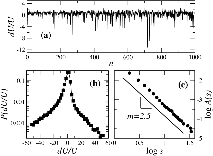
Figure 2: (a) Evolution of the variation of the total internal energy, which shows (b) probability density function and (c) avalanche size distribution similar to the ones observed for empirical data (compare with Fig. 1). Here $N=1000$, $K_{0}=1$ and $W_{ij}=1$ for all $i$ and $j$.

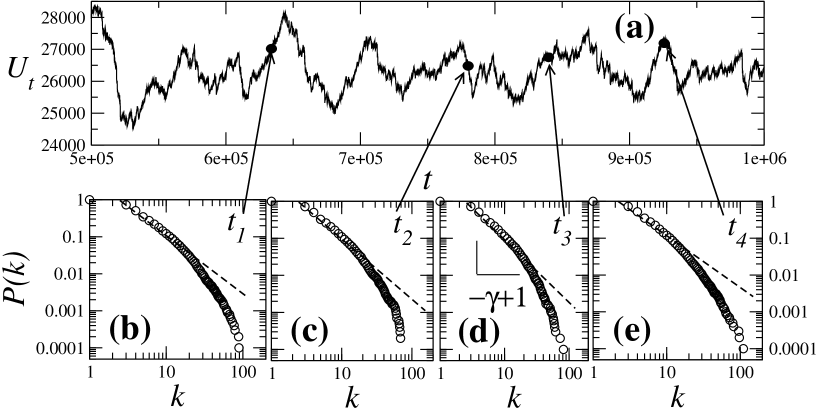
Figure 3: (a) Time series of the total internal energy $U$ of the agents. For the four instants $t_{1}$, $t_{2}$, $t_{3}$ and $t_{4}$ we show the observed cumulative degree distribution $P(k^{\ast}\geq k)\propto k^{-\gamma+1}$ yielding exponents (b) $\gamma=2.6\pm 0.5$, (c) $\gamma=2.7\pm 0.5$, (d) $\gamma=2.6\pm 0.5$, (e) $\gamma=2.6\pm 0.5$, all of them according to the theoretical prediction (check Eq. (8)). The deviations from the power-law for large $k$ are due to the avalanches (crisis) in the system (see text).

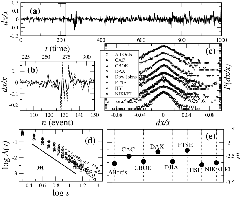
Figure 4: (a) Time evolution of the logarithmic returns of the DJIA index (partial). The box is zoomed in (b) to emphasize the contrast between real data (solid line) throughout time $t$ and the succession of events (dashed line) where the variation changes sign. (c) Probability density functions for some important financial indices, including interest rate options (CBOE). (d) Distribution of avalanche sizes detected throughout the evolution of each financial index showing critical behavior with (e) an exponent $m$ approximately invariant and similar to the one obtained for branching processes and to our model.

To know if one collapsing agent triggers an avalanche one needs to estimate the expected number of neighbors that the agent brings to collapse, due to its own collapse. If this expected number would be smaller than one, the systems would need to consume an infinite amount of energy from the environment. If the expected number would be larger than one, the entire system would typically be extinct by one large avalanche. The avalanche of collapsing agents form a branching process and assuming that the system cannot consume an infinite amount of energy from the environment and that the system survives the avalanches, the expected value of collapsing agents from a starting one must be equal to one[20] and therefore

$$\sum_{k_{in,i}=1}^{\infty}{k_{in,i}P(k_{in,i})P_{br}(k_{in,i})}=1$$ (6)

which yields $\sum_{k_{in,i}=1}^{\infty}{k_{in,i}^{-\gamma}}=\left(\frac{\omega}{K_{0}}\right)^{\gamma}$, i.e. the system remains in the critical state[20] as

$$\omega^{\gamma}=K_{0}^{\gamma}\zeta(2\gamma-1)$$ (7)

where $\zeta$ is the Riemann zeta-function. Condition (7) closes our model, relating economic growth ($K_{0}$), topology ($\gamma$) and the allowed level of debt($\omega$). From Otter’s theorem[21] for branching processes the distribution for the avalanche size expressed as number of agents $r$ is given by $P(r)\propto r^{-\frac{3}{2}}$. Since the energy of our system is expressed as connection number, the number of collapsed agents in an avalanche is given by $r=NK_{0}(\omega k_{in}))^{-\gamma}$, where $N$ is the total number of agents in the system. Therefore, the degree distribution is given by $P(k)\propto k^{-\frac{3}{2}\gamma}$ and the avalanche size distribution reads

$$P(k\geq s)\propto\int_{s}^{+\infty}{k^{-\frac{3}{2}\gamma}dk}\propto s^{-\frac{3}{2}\gamma+1}\equiv s^{-m}.$$ (8)

Equation (8) relates the exponent characterizing the network topology with the exponent taken from the avalanches, using first principles in economy theory.

Next we show that for the typical values of $\gamma$ found in empirical networks, our model reproduces the values of $m$ predicted in Eq. (8). For that, we define a macroscopic quantity for the internal energy, which accounts for all outgoing connections in the system at each time step:

$$U=\sum_{i=1}^{N}{\sum_{j\in{\cal V}_{out,i}}}{(W_{ij}-E_{ij})}.$$ (9)

The quantity $U$ varies through time, and its evolution reflects the development or fail of the underlying economy, similar to a finance index. Alternatively, $U$ can be calculated from the incoming connections. This macroscopic quantity will be used to characterize the state of our economic-like system.

Figure 2a shows a sketch of the evolution of a typical time-series for the logarithmic returns $dU/U$. As can be seen from Fig. 2b the distribution of the logarithmic returns is non-Gaussian with the heavy tails observed in empirical data[9]. In Fig. 2c the cumulative distribution $A(s)$ of the avalanche size $s$ is plotted showing a power-law whose fit yields $A(s)\sim s^{-m}$ with an exponent $m=2.51$ ($R^{2}=0.99$). Looking again to Eq. (8) and borrowing from the literature[17] the values of $\gamma$ of empirical networks which lay typically in the interval $[2.1,2.7]$, one concludes that the exponent should take typical values $m\in[2.15,3.05]$ which agrees with the results from our model.

Figure 3 shows how the overall index dynamic emerges from the underlying network mechanics. As agents connect each other by preferential attachment, the topology of the system is pushed to a power law degree distribution. On the other hand, avalanches push the system away from it. Thus, the system undergoes a structural fluctuation that generates a fat tail distribution of the index, expressed by Eq. (8) and shown in Fig. 4, rather than a Gaussian one. Figure 3a shows a typical set of successive $U_{t}$ values taken from our model. The cumulative degree distribution $P(k)$ at the marked instants $t_{1}$-$t_{4}$ are shown in Fig. 3b-3e. The dashed lines guide the eye for the scaling behavior observed at the lower part of the degree spectrum. In all cases $\gamma\sim 2.6$. Varying the threshold one observes other values for exponent $\gamma$ (not shown). For large degree $k$ the distribution deviates from the power-law, due to the drops of connections for agents experiencing an economical crash. Nonetheless, the slope $-\gamma+1$ of the dashed line yields values in the predicted range, within numerical errors.

Next we address the observation that the results obtained from our model in Fig. 2 do agree with the analysis done on eight main financial indices, as shown in Fig. 4.

The time-series of the logarithmic returns (Fig. 4a) must first be mapped in a series of events. One event is defined as a (typically small) set of successive instants in the original time-series having the same derivative sign, either positive (monotonically increasing values) or negative (monotonically decreasing values). Each time the derivative changes sign a new event starts. Figure 4b shows an zoom of the original time series in Fig. 4a (solid line) with the corresponding series of events. In the continuous limit, events would correspond to the instants in the time-series with vanishing first-derivative. Further, to be comparable to empirical series, we consider in our analysis a sampling of data which takes one measure of the original series from the system each five iterations.

The non-Gaussian distributions of the logarithmic returns (Fig. 4c) were extracted from the logarithm returns of the original series of each index, as in Ref. [9]. The characteristic heavy tails observed in [9] are observed for short time lag (hours or smaller), where in Fig. 4c the daily closure values are considered. The power-law behavior of the avalanche size (Fig. 4d) is indeed similar to the simulated results. Moreover the exponents $m$ have all approximate values, plotted in Fig. 4e, around the simulated value $m=2.51$ (solid line), and predicted by Eq. (8).

All empirical indices are sampled daily but in different time periods. For FTSE $6498$ days in London stock market were considered, starting on April 2nd 1984 and ending on December 18th 2009. For DJIA $20395$ days in New York stock market were considered, starting on October 1st and ending on December 18th 2009. For DAX $4815$ days in Frankfurt stock market were considered, starting on November 26th 1990 and ending on December 18th 2009. For CAC $5003$ days in Paris stock market were considered, starting on March 5th 1990 and ending on December 18th 2009. For ALLORDS $6555$ days in Australian stock market were considered, starting on August 3rd 1984 and ending on June 30th 2010. For HSI $5701$ days were considered in Hong Kong stock market, starting on December 31st 1986 and ending on December 18th 2009. For NIKKEI $6386$ days were analyzed in Tokyo stock market, starting on January 4th 1984 and ending on December 18th 2009. For CBOE IR10Y $12116$ days in Chicago derivative market, starting on January 2nd 1962 and ending on June 30th 2010.

4 Conclusions

In this paper, we have showed that, based only on first principles of economic theory and assuming that agents form an open system of economic connections organized by preferential attachment mechanisms, one is able to reach the distribution of drops observed in financial markets indices, including stocks and interest rate options. Assuming that the preferential attachment mechanism is part of the growing of economic connections, the resulting self-similar topology allows us to assume that the total economy system may present a similar topological structure as the sub-economy around financial markets and, thus, market indices can be taken as good proxies for the total economy.

We presented evidence that the distribution of drops in financial indices reflects the degree distribution taken from the trading network of the economical agents. In other words, the topology and structure of economic-like networks strongly influences the frequency and amplitude of economical crisis. Quantitatively, we showed that the two exponents characterizing the degree distribution and the distribution of drops, respectively, obey a scaling relation. Further, we showed how the scaling relation can be derived from a mean-field approach, assuming that the avalanche is a branching process of the economical agents and measuring its amplitude from the expected number of trading connections that are lost.

It should be noticed that the mean-field approach does not provide insight on local variations of both exponents. Differences between the different indices are also related to the different social-economic realities beneath them, including e.g. growing periods or crisis. For example, despite the fact that, in general, all economies have the same behavior, during a growing period the structure of the economic network shows a broader degree distribution (see e.g. Fig. 3e) corresponding to a higher value of the proxy (financial index).

The results averaged for sufficiently long time show that the numerical model here introduced reproduces the exponent $m\sim 5/2$ for the distribution of the drops observed in empirical financial indices. The value of the exponent $m$ gives indications of how large are crisis in the corresponding economy. Subsequent work that we are now finishing and will publish elsewhere shows that the exponent m is bounded by $[2,3.5]$.

Two final remarks are due here. First, as stated in the introduction, we only dealt with drops, occurring for a lower threshold of the difference between consumption and production at one single agent. Though, the interpretation of the total “energy” in the system as a financial index for the market can only be closed if the so-called “booms” are also considered in the evolution of the financial proxy. The booms were not incorporated in our model, since we were concerned with risk management. To incorporate them an additional threshold in the consumption would be needed.

Second, our results show that the full topology underlying economic-like systems plays an important role in the evolution of the proxies characterizing the economical state. In the particular context of financial networks, one may rise the question of how successful are directives and policies, such as Basel III, when they aim to avoid crisis through directives such as increasing minimum capital level in each financial agent. By translating this minimum capital level as a local threshold for each agent of a financial network, our model can be adapted to simulate future scenarios of the overall financial stability subjected to different thresholds. We have show that surprisingly the raise of such capital levels could drive the entire financial system into a state where larger crisis are more probable. This application of the model here introduced will be described in detail elsewhere[24], with a thorough discussion of the results.

References

- [1] F. Black, M. Scholes, J. of Polit. Econ. 81, 637 (1973); R.C. Merton, Bell J. of Econ. Manag. Sci. 4 (1973).
- [2] H.M. Markowitz, The Journal of Finance 7, 77 (1952).
- [3] O. Vasicek, J. of Fin. Economics. 5, 177 (1977).
- [4] O. Vasicek, “Distribution of Loan Portfolio Value” available at http://www.moodyskmv.com/conf04/pdf/papers/ dist_loan_port_val.pdf.
- [5] R. Friedrich, J. Peinke, and Ch. Renner, Phys. Rev. Lett. 84, 5224 (2000).
- [6] S. Ghashghaie, W. Breymann, J. Peinke, P. Talkner, Y. Dodge, Nature (London) 381, 767 (1996).
- [7] B. Mandelbrot, R. Hudson, The (mis)Behavior of Markets - A Fractal View of Risk, Ruin, and Reward, (Basic Books, USA, 2004).
- [8] R.N. Mantegna, H.E. Stanley Nature 376:46-49 (1995).
- [9] K. Kiyono, Z.R. Struzik, and Y. Yamamoto, Phys. Rev. Lett. 96, 068701 (2006).
- [10] P. Bak, C. Tang and K. Wiesenfeld, Phys. Rev. Lett. 59 381 (1987).
- [11] P. Bak and K. Sneppen, Phys. Rev. Lett. 71 4083 (1993).
- [12] B. Gutenberg and C.F. Richter, Seismicity of the Earth and Associated Phenomena, (Princeton Uni. Press, Princeton, 1954).
- [13] T. Lux and M. Marchesi, Nature 397 498 (1999).
- [14] E. Samanidou, E. Zschischang, D. Stauffer and T. Lux, Rep. Prog. Phys. 70 409 (2007).
- [15] S. Moss, Colloquium, PNAS 99 7267 (2002).
- [16] R. Lipsey and P. Steyner Economics (Harper & Row, USA, 1981).
- [17] A.-L. Barabási, R. Albert, Rev. Mod. Phys. 74 1 (2002).
- [18] J. von Neumann, The Rev. Econ. Studies 13, 1 (1945).
- [19] R.C.- Merton, J. Finance 29 449 (1974).
- [20] T.E. Harris, The Theory of Branching Processes (SpringerVerlag, Germany, 1963).
- [21] R. Otter, Annals of Mathematical Statistics 49 206 (1949).
- [22] M.J. Alava, P.K.V.V. Nukala and S. Zapperi, Adv. Phys. 55 349 (2006).
- [23] Y. Zhang, G.H.T. Lee, J.C. Wong, J.L. Kok, M. Prusty, and S.A. Cheong, Physica A 390(11) 2020-2050 (2011).
- [24] J.P. da Cruz and P.G. Lind, “The dynamics of financial stability”, submitted, 2011; available at http://arxiv.org/abs/1103.0717.