Gamma-convergence results for phase-field approximations of the 2D-Euler Elastica Functional

Abstract.

We establish some new results about the $\Gamma$-limit, with respect to the $L^{1}$-topology, of two different (but related) phase-field approximations of the so-called Euler’s Elastica Bending Energy for curves in the plane.

1. Introduction

In this paper we present some new results about the sharp interface limit of two sequences of phase-field functionals involving the so-called Cahn-Hilliard energy functional and its $L^{2}$-gradient. The study of this kind of problems is motivated by applications in different fields ranging from image processing (e.g., [17, 25, 8, 5]), to the diffuse interface approximation of elastic bending energies (e.g., [14, 15, 16, 26, 3, 7]), to the study of singular limits of partial differential equations and systems (e.g., [32, 29, 24, 34]), up to the study of rare events for stochastic perturbations of the so-called Allen-Cahn equation (e.g., [22, 30]).

Let us now introduce the two sequences of energies we wish to study. Given $\Omega\subset\mathbb{R}^{d}$ open, bounded and with smooth boundary, we define the so-called Cahn-Hilliard energy by

$$\mathcal{P}_{\varepsilon}(u):=\begin{cases}\int_{\Omega}\frac{\varepsilon}{2}|\nabla u|^{2}+\frac{W(u)}{\varepsilon}\,dx&\text{if }u\in W^{1,2}(\Omega),\\ +\infty&\text{otherwise on }L^{1}(\Omega)\end{cases}$$ (1.1)

where $\varepsilon>0$ is a parameter representing the typical “diffuse interface width”, and $W\in C^{3}(\mathbb{R},\mathbb{R}^{+}\cup\{0\})$ is a double-well potential with two equal minima (throughout the paper we make the choice $W(s):=(1-s^{2})^{2}/4$, though most of the results we obtain hold true for a wider class of potentials). The sequences of functionals $\{\widetilde{\mathcal{E}}_{\varepsilon}\}_{\varepsilon},\,\{\mathcal{E}_{\varepsilon}\}_{\varepsilon}$ we consider in this paper are respectively defined by

$$\widetilde{\mathcal{E}}_{\varepsilon}:=\mathcal{P}_{\varepsilon}+\mathcal{W}_{\varepsilon}:\,L^{1}(\Omega)\to\,[0,+\infty],$$ (1.2)

$$\text{ where }\mathcal{W}_{\varepsilon}(u):=\begin{cases}\frac{1}{\varepsilon}\int_{\Omega}\Big{(}\varepsilon\Delta u-\frac{W^{\prime}(u)}{\varepsilon}\Big{)}^{2}\,dx&\text{if }u\in W^{2,2}(\Omega)\\ +\infty&\text{elsewhere on }L^{1}(\Omega),\end{cases},$$ (1.3)

and

$$\mathcal{E}_{\varepsilon}:=\mathcal{P}_{\varepsilon}+\mathcal{B}_{\varepsilon}:\,L^{1}(\Omega)\to\,[0,+\infty],$$ (1.4)

$$\text{where }\mathcal{B}_{\varepsilon}(u):=\begin{cases}\frac{1}{\varepsilon}\int_{\Omega}\Big{|}\varepsilon\nabla^{2}u-\frac{W^{\prime}(u)}{\varepsilon}\nu_{u}\otimes\nu_{u}\Big{|}^{2}\,dx&\text{if }u\in W^{2,2}(\Omega)\\ +\infty&\text{elsewhere on }L^{1}(\Omega)\end{cases},$$ (1.5)

and $\nu_{u}$ is a unit vector-field such that

$$\nu_{u}=\frac{\nabla u}{|\nabla u|}\,\text{on }\{\nabla u\neq 0\}\text{ and }\nu_{u}\equiv const.\,\text{on }\{\nabla u=0\}.$$

We remark that $\mathcal{W}_{\varepsilon}(u)$ represents the (rescaled) norm of the $L^{2}$-gradient of $\mathcal{P}_{\varepsilon}$ at $u$, and that $\mathcal{W}_{\varepsilon}$ and $\mathcal{B}_{\varepsilon}$ are linked by the relation

$$\mathrm{tr}\Big{[}\varepsilon\nabla^{2}u-\frac{W^{\prime}(u)}{\varepsilon}\nu_{u}\otimes\nu_{u}\Big{]}=\varepsilon\Delta u-\frac{W^{\prime}(u)}{\varepsilon}.$$

Hence, denoted by $\{\lambda_{1},\dots,\lambda_{d}\}$ the eigenvalues of the symmetric $d\times d$-matrix $\varepsilon\nabla^{2}u-(W^{\prime}(u)/\varepsilon)\nu_{u}\otimes\nu_{u}$, we have

$$d\Big{(}\sum_{i=1}^{d}\lambda_{i}^{2}\Big{)}=d\left|\varepsilon\nabla^{2}u-\frac{W^{\prime}(u)}{\varepsilon}\nu_{u}\otimes\nu_{u}\right|^{2}\geq\left(\varepsilon\Delta u_{\varepsilon}-\frac{W^{\prime}(u_{\varepsilon})}{\varepsilon}\right)^{2}=\Big{(}\sum_{i=1}^{d}\lambda_{i}\Big{)}^{2}.$$ (1.6)

Next, we briefly summarize the known results about the sharp interface limit of $\{\widetilde{\mathcal{E}}_{\varepsilon}\}_{\varepsilon}$ and $\{\mathcal{E}_{\varepsilon}\}_{\varepsilon}$. The starting point for the analysis of the asymptotic behavior, as $\varepsilon\to 0$, of the sequences $\{\widetilde{\mathcal{E}}_{\varepsilon}\}_{\varepsilon},\,\{\mathcal{E}_{\varepsilon}\}_{\varepsilon}$ is a well-known result, due to Modica and Mortola, establishing the $\Gamma$-convergence of $\mathcal{P}_{\varepsilon}$ to the area functional. More precisely in [28] it has been proved that the $\Gamma(L^{1}(\Omega))$-limit of the sequence $\{\mathcal{P}_{\varepsilon}\}_{\varepsilon}$ is given by

$$\Gamma(L^{1}(\Omega))-\lim_{\varepsilon\to 0}\mathcal{P}_{\varepsilon}(u)=\mathcal{P}(u):=\begin{cases}\frac{c_{0}}{2}\int_{\Omega}\,d|\nabla u|&\text{if }u\in BV(\Omega,\{-1,1\}),\\ +\infty&\text{elsewhere in }L^{1}(\Omega)\end{cases}$$

where $c_{0}:=\int_{-1}^{1}\sqrt{2W(s)}\,ds$ (see Section 2.5 and Section 3 for further details). We remark that for every $u\in BV(\Omega,\{-1,1\})$ we can write $u=2\chi_{E}-1=:\mathbbm{1}_{E}$, where $\chi_{E}$ denotes the characteristic function of the finite perimeter set $E:=\{u\geq 1\}$. Hence $\mathcal{P}(u)=c_{0}\mathcal{H}^{d-1}(\partial^{*}E)$ where $\mathcal{H}^{d-1}$ denotes the $(d-1)$-dimensional Hausdorff measure in $\mathbb{R}^{d}$ and $\partial^{*}E$ denotes the reduced boundary of $E$ (see [35]).

The main result concerning the $\Gamma$-convergence of $\{\widetilde{\mathcal{E}}_{\varepsilon}\}_{\varepsilon}$ has been established, for $d=2$ and $d=3$, by Röger and Schätzle in [31] and independently, but only in the case $d=2$, by Tonegawa and Yuko in [36], partially answering to a conjecture of De Giorgi (see [11]). In particular in [31] the authors proved that for $d=2$ or $3$ and $u=\mathbbm{1}_{E}\in BV(\Omega,\{-1,1\})$ such that $E\subset\Omega$ is open and $\Omega\cap\partial E\in C^{2}$, we have

$$\Gamma(L^{1}(\Omega))-\lim_{\varepsilon\to 0}\widetilde{\mathcal{E}}_{\varepsilon}(u)=c_{0}\int_{\Omega\cap\partial E}\big{[}1+|\mathbf{H}_{\partial E}(x)|^{2}]\,d\mathcal{H}^{d-1}(x),$$ (1.7)

where $\mathbf{H}_{\partial E}(x)$ denotes the mean curvature vector of $\partial E$ in the point $x\in\partial E$. When $d=2$ we call the functional on the right hand side of (1.7) the Euler’s Elastica Functional.

The sequence of functionals $\{\mathcal{E}_{\varepsilon}\}_{\varepsilon}$ has been introduced in [3] in connection with the problem of finding a diffuse interface approximation of the Gaussian curvature. As a straightforward consequence of the results established in [3] it follows that, again for $d=2,3$ and $u=\mathbbm{1}_{E}\in BV(\Omega,\{-1,1\})$ such that $E\subset\Omega$ is open and $\Omega\cap\partial E\in C^{2}$, we have

$$\Gamma(L^{1}(\Omega))-\lim_{\varepsilon\to 0}\mathcal{E}_{\varepsilon}(u)=c_{0}\int_{\Omega\cap\partial E}[1+|\mathbf{B}_{\partial E}(x)|^{2}]\,d\mathcal{H}^{d-1}(x),$$ (1.8)

where this time $\mathbf{B}_{\partial E}(x)$ denotes the second fundamental form of $\partial E$ in the point $x\in\partial E$.

In the present paper we restrict to the case $d=2$, and investigate the behavior of $\{\widetilde{\mathcal{E}}_{\varepsilon}\}_{\varepsilon}$ and $\{\mathcal{E}_{\varepsilon}\}_{\varepsilon}$ along sequences $\{u_{\varepsilon}\}_{\varepsilon}\subset C^{2}(\Omega)$ such that

$$L^{1}(\Omega)-\lim_{\varepsilon\to 0}u_{\varepsilon}=\mathbbm{1}_{E}\in BV(\Omega,\{-1,1\}),$$ (1.9)

removing the regularity assumption on the limit set $E$. In other words we aim to prove a full $\Gamma$-convergence result, on the whole space $L^{1}(\Omega)$.

We recall that if a sequence of functionals $\Gamma$-converges, and a certain equicoercivity property holds, then the minimizers of such sequence converge to the minimizers of the $\Gamma$-limit. Therefore, besides its possible mathematical interest, we expect that a description of the $\Gamma$-limit may be of some relevance at least for those applications, such as [5, 13, 14, 15, 3, 26], where the sequences $\{\widetilde{\mathcal{E}}_{\varepsilon}\}_{\varepsilon}$ and $\{\mathcal{E}_{\varepsilon}\}_{\varepsilon}$ are introduced to formulate, and solve numerically, a “diffuse interface” variational problem whose solutions are expected to converge, as $\varepsilon\to 0$, to the solutions of a given sharp interface minimum problem.

In synthesis our result says that the sharp interface limits of $\{\widetilde{\mathcal{E}}_{\varepsilon}\}_{\varepsilon}$ and $\{\mathcal{E}_{\varepsilon}\}_{\varepsilon}$ in general do not coincide out of “smooth points”, although in two space dimensions, by (1.7) and (1.8) and

$$|\mathbf{B}_{\partial E}(x)|^{2}=|\mathbf{H}_{\partial E}(x)|^{2},$$ (1.10)

we have, for $u=\mathbbm{1}_{E}$ and $E\subset\Omega$ open such that $\Omega\cap\partial E\in C^{2}$,

$$\Gamma(L^{1}(\Omega))-\lim_{\varepsilon\to 0}\mathcal{E}_{\varepsilon}(u)=\Gamma(L^{1}(\Omega))-\lim_{\varepsilon\to 0}\widetilde{\mathcal{E}}_{\varepsilon}(u).$$

More precisely we prove that, in accordance with (1.6), we have

$$\Gamma(L^{1}(\Omega))-\lim_{\varepsilon\to 0}\widetilde{\mathcal{E}}_{\varepsilon}(u)\leq\Gamma(L^{1}(\Omega))-\lim_{\varepsilon\to 0}\mathcal{E}_{\varepsilon}(u)$$

and that there are functions $u\in BV(\Omega,\{-1,1\})$ for which the above inequality is strict. In fact we show that, on one hand, a uniform bound on $\mathcal{E}_{\varepsilon}(u_{\varepsilon})$ implies that the energy density measures

$$\mu_{\varepsilon}:=c_{0}^{-1}[\varepsilon/2|\nabla u_{\varepsilon}|^{2}+W(u_{\varepsilon})/\varepsilon]\mathcal{L}^{d}_{\mathop{\hbox{\vrule height=7.0pt,width=0.5pt,depth=0.0pt\vrule height=0.5pt,width=6.0pt,depth=0.0pt}}\nolimits\Omega}$$

(here $\mathcal{L}^{d}$ denotes the Lebesgue measure on $\mathbb{R}^{d}$) concentrate on a set whose tangent cone in every point is given by an unique tangent line. On the other hand we show that a uniform bound on $\widetilde{\mathcal{E}}_{\varepsilon}(u_{\varepsilon})$ allows the energy measures to concentrate on cross-shaped sets. This difference in regularity between the support of the two limit measures is related to the existence of so called “saddle shaped solutions” to the semilinear elliptic equation $-\Delta U+W^{\prime}(U)=0$ on $\mathbb{R}^{2}$ (see [10, 6, 12], and the proof of Theorem 4.5 in this paper).

To give a better description of our results, let us briefly explain the role played by the regularity assumption on the limit set $E$ in the proofs of (1.7) and (1.8), and discuss the obstructions to remove such an assumption. To this aim, for the readers convenience, we briefly recall the backbone of the proof of (1.7) (and point out that the proof (1.8) follows the same line of arguments).

To prove (1.7) one has to find a lower-bound for $\widetilde{\mathcal{E}}_{\varepsilon}(u_{\varepsilon})$ proving the so-called $\Gamma-\liminf$ inequality; and to show that such lower-bound is in a way “optimal” via the so-called $\Gamma-\limsup$ inequality. (See Section 2.5 for a precise definition of $\Gamma$-convergence).

Let us begin recalling how the $\Gamma-\liminf$ inequality has been proved. Suppose that $\{u_{\varepsilon}\}_{\varepsilon}\subset C^{2}(\Omega)$ verifies (1.9) and

$$\sup_{\varepsilon>0}\widetilde{\mathcal{E}}_{\varepsilon}(u_{\varepsilon})<+\infty.$$ (1.11)

Thanks to the bound (uniform in $\varepsilon$) on $\mathcal{P}_{\varepsilon}(u_{\varepsilon})$ and the convergence of $u_{\varepsilon}$ to $u$, applying the results of [28] it can be easily deduced that (up to subsequences) the energy-density measures $\mu_{\varepsilon}$ defined above converge to a Radon measure $\mu$ in $\Omega$ such that $\mathcal{H}^{d-1}_{\mathop{\hbox{\vrule height=7.0pt,width=0.5pt,depth=0.0pt\vrule height=0.5pt,width=6.0pt,depth=0.0pt}}\nolimits\partial^{*}E}<<\mu.$ That is, roughly speaking, the support of $\mu$ contains the (reduced) boundary of $E$. In case only a bound on $\mathcal{P}_{\varepsilon}(u_{\varepsilon})$ is available, there is no much hope to obtain more informations about the measure $\mu$, since this latter may be quite irregular (for example it may contain parts that are absolutely continuous with respect to $\mathcal{L}^{d}$). However when (1.11) holds, the bound on $\mathcal{W}_{\varepsilon}(u_{\varepsilon})$ implies that $\mu$ has some “weak” regularity properties. In fact the first crucial step in the derivation of a lower bound for $\widetilde{\mathcal{E}}_{\varepsilon}(u_{\varepsilon})$ consists in proving that (1.11) guarantees that:

• the measure $\mu$ has the form $\mu=\theta\,\mathcal{H}^{d-1}_{\mathop{\hbox{\vrule height=7.0pt,width=0.5pt,depth=0.0pt\vrule height=0.5pt,width=6.0pt,depth=0.0pt}}\nolimits M}$, where $M$ is a generalized hypersurface of $\mathbb{R}^{d}$, and $\theta:M\to\mathbb{N}$ is an integer valued $\mathcal{H}^{d-1}_{\mathop{\hbox{\vrule height=7.0pt,width=0.5pt,depth=0.0pt\vrule height=0.5pt,width=6.0pt,depth=0.0pt}}\nolimits M}$ -measurable function;

• a generalized mean curvature vector $\mathbf{H}_{\mu}\in L^{2}(\mu)$ is well defined $\mu$-a.e.;

• the following relation holds

  $$\liminf_{\varepsilon\to 0}\widetilde{\mathcal{E}}_{\varepsilon}(u_{\varepsilon})\geq c_{0}\int[1+|\mathbf{H}_{\mu}|^{2}]\,d\mu.$$ (1.12)

(Namely, $\mu$ is the weight measure of an integral rectifiable varifold with $L^{2}$-bounded first variation, see Section 2.3 for some basic facts and terminology about varifolds theory).

The next step in the proof of the $\Gamma-\liminf$-inequality consists in relating the generalized mean curvature vector $\mathbf{H}_{\mu}$ of $\mu$ with the (generalized) mean curvature vector of the phase-boundary $\partial^{*}E$. Since $\mathcal{H}^{d-1}_{\mathop{\hbox{\vrule height=7.0pt,width=0.5pt,depth=0.0pt\vrule height=0.5pt,width=6.0pt,depth=0.0pt}}\nolimits\partial^{*}E}<<\mu$, by the results of [27] (see also [33, 23]) it follows that $\partial^{*}E$ can be covered with the union of a countable family of $(d-1)$-dimensional $C^{2}$-manifolds embedded in $\mathbb{R}^{d}$, and with a set of $\mathcal{H}^{d-1}$-measure zero. Hence the mean curvature vector $\mathbf{H}_{\partial^{*}E}$ of $\partial^{*}E$ is well defined $\mathcal{H}^{d-1}_{\mathop{\hbox{\vrule height=7.0pt,width=0.5pt,depth=0.0pt\vrule height=0.5pt,width=6.0pt,depth=0.0pt}}\nolimits\partial^{*}E}$-a.e. Furthermore by [27] (see also [23, 33] and Remark 2.2) we have $\mathbf{H}_{\mu}(x)=\mathbf{H}_{\partial^{*}E}(x)$ for $\mathcal{H}^{d-1}$-a.e. $x\in\partial^{*}E$ . Eventually, being $\mathcal{H}^{d-1}_{\mathop{\hbox{\vrule height=7.0pt,width=0.5pt,depth=0.0pt\vrule height=0.5pt,width=6.0pt,depth=0.0pt}}\nolimits\partial^{*}E}<<\mu$ and $\theta(x)\geq 1$ for $\mu$-a.e. $x\in M$, by (1.12) it follows that

$$\liminf_{\varepsilon\to 0}\widetilde{\mathcal{E}}_{\varepsilon}(u_{\varepsilon})\geq c_{0}\int[1+|\mathbf{H}_{\mu}|^{2}]\,d\mu\geq c_{0}\int_{\Omega\cap\partial^{*}E}[1+|\mathbf{H}_{\partial^{*}E}|^{2}]\,d\mathcal{H}^{d-1}.$$ (1.13)

It remains to establish if (or when) such a lower bound is “optimal”. More precisely, it remains to understand for which $u=\mathbbm{1}_{E}\in BV(\Omega,\{-1,1\})$ is it possible to find a “ recovery sequence” $\{u_{\varepsilon}\}_{\varepsilon}\subset C^{2}(\Omega)$, that is a sequence such that

$$\lim_{\varepsilon\to 0}u_{\varepsilon}=u\text{ in }L^{1}(\Omega)\text{ and }\limsup_{\varepsilon\to 0}\widetilde{\mathcal{E}}_{\varepsilon}(u_{\varepsilon})\leq c_{0}\int_{\Omega\cap\partial^{*}E}[1+|\mathbf{H}_{\partial^{*}E}|^{2}]\,d\mathcal{H}^{d-1}.$$ (1.14)

For those $u$ it follows that

$$\Gamma(L^{1}(\Omega))-\lim_{\varepsilon\to 0}\widetilde{\mathcal{E}}_{\varepsilon}(u_{\varepsilon})=c_{0}\int_{\partial^{*}E\cap\Omega}[1+|\mathbf{H}_{\partial^{*}E}|^{2}]\,d\mathcal{H}^{d-1}$$ (1.15)

(in fact (1.13) and (1.14) respectively represent the $\Gamma-\liminf$ and the $\Gamma-\limsup$-inequality). When $E\subset\Omega$ and $\Omega\cap\partial E\in C^{2}$, it is relatively easy to construct a sequence $\{u_{\varepsilon}\}_{\varepsilon}\subset C^{2}(\Omega)$ verifying (1.14) (see [4]), and this concludes the proof of (1.7).

Actually, by a simple diagonal argument, we can construct a sequence $\{u_{\varepsilon}\}_{\varepsilon}\subset C^{2}(\Omega)$ verifying (1.14) (and consequently obtain that (1.15) holds true) for all those functions $u=\mathbbm{1}_{E}\in BV(\Omega,\{-1,1\})$ for which there exists a sequence $\{E_{h}\}_{h}$ such that $E_{h}\subset\Omega$ is open and $\Omega\cap\partial E_{h}\in C^{2}$ for every $h\in\mathbb{N}$, and such that

$$\lim_{h\to\infty}\mathbbm{1}_{E_{h}}=u\text{ in }L^{1}(\Omega),\quad\lim_{h\to\infty}\int_{\Omega\cap\partial E_{h}}[1+|\mathbf{H}_{\partial E_{h}}|^{2}]\,d\mathcal{H}^{d-1}=\int_{\Omega\cap\partial E}[1+|\mathbf{H}_{\partial E}|^{2}]\,d\mathcal{H}^{d-1}$$

(e.g., if $E\subset\Omega$ is open and $\Omega\cap\partial E\in W^{2,2}$, see Remark 2.14).

As we already said (1.8) is obtained following a similar line of arguments.

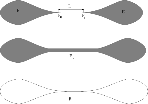
Figure 1. The set $E\subset\subset\Omega$ has smooth boundary out of the two sharp cusps $p_{0},\,p_{1}$, that are aligne and placed at a distance $L>0$. The first variation of the rectifiable varifold $\widehat{V}=\mathbf{v}(\partial^{*}E,1)$ associated to $\widehat{\mu}:=\mathcal{H}^{1}_{\mathop{\hbox{\vrule height=7.0pt,width=0.5pt,depth=0.0pt\vrule height=0.5pt,width=6.0pt,depth=0.0pt}}\nolimits\partial^{*}E}$ is given by $\delta\widehat{V}=\mathbf{H}_{\partial^{*}E}\mathcal{H}^{1}_{\mathop{\hbox{\vrule height=7.0pt,width=0.5pt,depth=0.0pt\vrule height=0.5pt,width=6.0pt,depth=0.0pt}}\nolimits\partial^{*}E}+2\sum_{j=0,1}\mathbf{e}_{1}(-1)^{j}\delta_{p_{j}}$, where $\mathbf{e}_{1}=(1,0)\in\mathbb{R}^{2}$ and $\delta_{p_{j}}$ is the Dirac-delta at $p_{j}$. Hence $\delta\widehat{V}\notin[L^{2}(\widehat{\mu})]^{*}$, see Section 2.3. For every $h\in\mathbb{N}$ the set $E_{h}$, such that $E_{h}\subset\subset\Omega$ and $\partial E_{h}\in C^{2}$, is obtained replacing $p_{0}$ and $p_{1}$ with a flat tubular neighborhood of height $1/h$ that approximates the segment connecting $p_{0}$ and $p_{1}$ as $h\to\infty$.

Yet we do not expect neither (1.15) nor its analogue for the $\Gamma(L^{1}(\Omega))-\lim_{\varepsilon\to 0}\mathcal{E}_{\varepsilon}(u)$ to be always true, as the following example suggests. Suppose that $E\subset\subset\Omega$ is as in Figure 1. We then have $u=\mathbbm{1}_{E}\in BV(\Omega,\{-1,1\})$. Moreover if we consider the sequence $\{E_{h}\}_{h}$ of smooth sets represented in Figure 1, we have

$$L^{1}(\Omega)-\lim_{h\to\infty}\mathbbm{1}_{E_{h}}=u,$$

$$\lim_{h\to\infty}\int_{\partial E_{h}}[1+|\mathbf{H}_{\partial E_{h}}|^{2}]\,d\mathcal{H}^{1}=\int[1+|\mathbf{H}_{\mu}|^{2}]\,d\mu=\int_{\partial^{*}E}[1+|\mathbf{H}_{\partial^{*}E}|^{2}]\,d\mathcal{H}^{1}+2L.$$

Hence, for every $u_{h}:=\mathbbm{1}_{E_{h}}$ ($h\in\mathbb{N}$), by [4, 3], we can construct a recovery sequence $\{u_{h,\varepsilon}\}_{\varepsilon}\subset C^{2}(\Omega)$. Then, by a diagonal argument, we can select a sequence $\{u_{\varepsilon}\}_{\varepsilon}\subset C^{2}(\Omega)$ such that $\lim_{\varepsilon\to 0}u_{\varepsilon}=u$ in $L^{1}(\Omega)$ and

$$\lim_{\varepsilon\to 0}\widetilde{\mathcal{E}}_{\varepsilon}(u_{\varepsilon})=\lim_{\varepsilon\to 0}\mathcal{E}_{\varepsilon}(u_{\varepsilon})=c_{0}\int_{\Omega\cap\partial^{*}E}[1+|\mathbf{H}_{\partial^{*}E}|^{2}]\,d\mathcal{H}^{1}+2c_{0}L<+\infty.$$

Therefore we can conclude that

$$\max\{\Gamma(L^{1}(\Omega))-\lim_{\varepsilon\to 0}\widetilde{\mathcal{E}}_{\varepsilon}(u),\,\Gamma(L^{1}(\Omega))-\lim_{\varepsilon\to 0}\mathcal{E}_{\varepsilon}(u)\}<+\infty.$$

For this choice of $u\in BV(\Omega,\{-1,1\})$ we expect that neither (1.15), nor its analogue for $\Gamma(L^{1}(\Omega))-\lim_{\varepsilon\to 0}\mathcal{E}_{\varepsilon}(u)$ hold. In fact: on the one hand (1.7) and (1.8) hold as soon as we localize the functionals $\widetilde{\mathcal{E}}_{\varepsilon}$ and $\mathcal{E}_{\varepsilon}$ on any open subset $\omega$ such that $\overline{\omega}\cap\{p_{0},p_{1}\}=\emptyset$; on the other hand we cannot have

$$\lim_{\varepsilon\to 0}\mu_{\varepsilon}=\mathcal{H}^{1}_{\mathop{\hbox{\vrule height=7.0pt,width=0.5pt,depth=0.0pt\vrule height=0.5pt,width=6.0pt,depth=0.0pt}}\nolimits\partial^{*}E}\text{ as Radon measures on }\Omega,$$

as this would contradict the fact (established in [31, 36, 3] and recalled above) that the rectifiable varifold associated with the limit of the $\mu_{\varepsilon}$ has $L^{2}$-bounded first variation. Hence we expect that for every sequence $\{u_{\varepsilon}\}_{\varepsilon}\subset C^{2}(\Omega)$ such that $u_{\varepsilon}\to u$ in $L^{1}(\Omega)$ we have

$$\frac{1}{c_{0}}\min\{\liminf_{\varepsilon\to 0}\widetilde{\mathcal{E}}_{\varepsilon}(u_{\varepsilon}),\,\liminf_{\varepsilon\to 0}\mathcal{E}_{\varepsilon}(u_{\varepsilon})\}\geq\int[1+|\mathbf{H}_{\mu}|^{2}]\,d\mu>\int_{\partial^{*}E}[1+|\mathbf{H}_{\partial^{*}E}|^{2}]\,d\mathcal{H}^{1},$$

that is the last term on the right hand side is a too rough (or “non-optimal”) lower-bound for both $\widetilde{\mathcal{E}_{\varepsilon}}(u_{\varepsilon})$ and $\mathcal{E}_{\varepsilon}(u_{\varepsilon})$. It is thus rather natural to try to answer the question: what are the $\Gamma$-limits of $\{\widetilde{\mathcal{E}}_{\varepsilon}\}_{\varepsilon}$ and $\{\mathcal{E}_{\varepsilon}\}_{\varepsilon}$ out of “smooth sets”?

We try to answer this question in the case $d=2$ only, and from now on, throughout the paper we will assume that $d=2$, unless otherwise specified.

Since $\Gamma$-limits are necessarily lower semi-continuous functionals (see [9, Proposition 4.16]), in view of (1.7), (1.8) and (1.10), a natural candidate for the $\Gamma$-limit of both $\widetilde{\mathcal{E}_{\varepsilon}}$ and $\mathcal{E}_{\varepsilon}$ is the lower semi-continuous envelope (with respect to the $L^{1}(\Omega)$-topology) of the functional

$$\mathcal{F}_{o}:L^{1}(\Omega)\to\,[0,+\infty],\quad u\mapsto\begin{cases}\int_{\Omega\cap\partial E}[1+|\mathbf{H}_{\partial E}|^{2}]\,d\mathcal{H}^{1}&\text{if }u=\mathbbm{1}_{E}\text{ and }\Omega\cap\partial E\in C^{2},\\ +\infty&\text{otherwise on }L^{1}(\Omega),\end{cases}$$

that is the functional

$$\overline{\mathcal{F}}_{o}(u):= \inf\{\liminf_{k\to\infty}\mathcal{F}_{o}(u_{k}):~{}L^{1}(\Omega)-\lim_{k\to\infty}u_{k}=u\}$$

$$= \sup\{\mathcal{G}(u):~{}\mathcal{G}\leq\mathcal{F}_{o}\text{ on }L^{1}(\Omega),\,\mathcal{G}\text{ is lower semi-continuous on }L^{1}(\Omega)\}.$$

Since by [1, Theorem 3.2] we have $\overline{\mathcal{F}}_{o}(u)=\mathcal{F}_{o}(u)$ for every $u=\mathbbm{1}_{E}$ such that $\Omega\cap\partial E\in W^{2,2}$ (see also [33] for a more general statement), by (1.7), (1.8) and the definition of $\overline{\mathcal{F}}_{o}$, we can conclude that

$$\Gamma(L^{1}(\Omega))-\lim_{\varepsilon\to 0}\widetilde{\mathcal{E}}_{\varepsilon}\leq c_{0}\overline{\mathcal{F}}_{o}\text{ on }L^{1}(\Omega),\quad\Gamma(L^{1}(\Omega))-\lim_{\varepsilon\to 0}\mathcal{E}_{\varepsilon}\leq c_{0}\overline{\mathcal{F}}_{o}\text{ on }L^{1}(\Omega).$$

We can now rephrase the results we obtain as follows: we prove that $\Gamma(L^{1}(\Omega))-\lim_{\varepsilon\to 0}\mathcal{E}_{\varepsilon}=c_{0}\overline{\mathcal{F}}_{o}$ (at least under suitable boundary conditions for the phase-field variable), and we show that in general $\Gamma(L^{1}(\Omega))-\lim_{\varepsilon\to 0}\widetilde{\mathcal{E}}_{\varepsilon}<c_{0}\overline{\mathcal{F}}_{o}$.

The outline of the paper is the following. In Theorem 4.1, we show that the assumption

$$\sup_{\varepsilon>0}\mathcal{E}_{\varepsilon}(u_{\varepsilon})<+\infty,$$

implies additional “regularity” on the support of the measure $\mu:=\theta\mathcal{H}^{1}_{\mathop{\hbox{\vrule height=7.0pt,width=0.5pt,depth=0.0pt\vrule height=0.5pt,width=6.0pt,depth=0.0pt}}\nolimits M}$ arising as limit of the energy density measures $\mu_{\varepsilon}$ defined above. Namely we establish that in every point of $M\cap\Omega$ a (unique) tangent-line to $M$ is well defined. Moreover, in Corollary 4.2, we show that if $\{u_{\varepsilon}\}_{\varepsilon}\subset X$ where

$$X:=\{u\in C^{2}(\Omega):~{}u(x)\equiv 1,\,\partial_{\nu_{\Omega}}u(x)=0,\,\forall x\in\partial\Omega\},$$

then the set $M\cup\partial\Omega$ has an uniquely defined tangent line in every point. In view of [2, 3] (see also Theorem 2.13 and Theorem 3.3 in this paper) this allows us to conclude that $\Gamma(L^{1}(\Omega))-\lim_{\varepsilon\to 0}\mathcal{E}_{\varepsilon\mathop{\hbox{\vrule height=7.0pt,width=0.5pt,depth=0.0pt\vrule height=0.5pt,width=6.0pt,depth=0.0pt}}\nolimits X}=c_{0}\overline{\mathcal{F}}$, where $\overline{\mathcal{F}}$ denotes the $L^{1}(\Omega)$-lower semi-continuos envelope of $\mathcal{F}_{o\mathop{\hbox{\vrule height=7.0pt,width=0.5pt,depth=0.0pt\vrule height=0.5pt,width=6.0pt,depth=0.0pt}}\nolimits\mathscr{K}}$ and

$$\mathscr{K}:=\{E\subset\Omega:~{}E\text{ is open, compactly contained in }\Omega\text{ and }\partial E\in C^{2}\}$$

(the restriction of $\mathcal{F}_{o}$ to $\mathscr{K}$ is a consequence of the fact that here we are considering the $\Gamma$-limit of $\mathcal{E}_{\varepsilon\mathop{\hbox{\vrule height=7.0pt,width=0.5pt,depth=0.0pt\vrule height=0.5pt,width=6.0pt,depth=0.0pt}}\nolimits X}$).

We remark that we do not expect that an analogoue of Theorem 4.1 holds in space dimensions $d>2$. In fact, to prove Theorem 4.1 we make use of a blow-up argument and of some regularity results obtained in [18], that are valid only for generalized $(d-1)$-dimensional hypersurfaces (namely, Hutchinson’s curvature varifolds) with $p$-integrable (generalized) second fundamental form for some $p>(d-1)$. Moreover, though we expect that an analogue of Corollary 4.2 holds also (at least) when $d=3$, to prove such a result we would probably need a different approach. In fact, in the proof of Corollary 4.2 we make an essential use of an “explicit” representation of $\overline{\mathcal{F}}$, that has been established in [2] and is available only in two space dimensions.

For what concerns the sequence $\{\widetilde{\mathcal{E}}_{\varepsilon}\}_{\varepsilon}$, in Theorem 4.5 we show that in general the support of the limit measure does not necessarily have an unique tangent line in every point, and we obtain the existence of a function $u=\mathbbm{1}_{E}\in BV(\Omega,\{-1,1\})$ such that

$$\Gamma(L^{1}(\Omega))-\lim_{\varepsilon\to 0}\widetilde{\mathcal{E}}_{\varepsilon}(u)<c_{0}\overline{\mathcal{F}}_{0}(u)=\Gamma(L^{1}(\Omega))-\lim_{\varepsilon\to 0}\mathcal{E}_{\varepsilon}(u)=+\infty.$$

This means that the sharp interface limit of $\mathcal{E}_{\varepsilon}$ and $\widetilde{\mathcal{E}}_{\varepsilon}$ do not coincide as functionals on $L^{1}(\Omega)$, although as we already remarked $\Gamma(L^{1}(\Omega))-\lim_{\varepsilon\to 0}\widetilde{\mathcal{E}}_{\varepsilon}(u)=\Gamma(L^{1}(\Omega))-\lim_{\varepsilon\to 0}\mathcal{E}_{\varepsilon}(u)$ whenever $u=\mathbbm{1}_{E}$ and $\Omega\cap\partial E\in C^{2}$.

Although we are not able to completely identify the $\Gamma(L^{1}(\Omega))-\lim_{\varepsilon\to 0}\widetilde{\mathcal{E}}_{\varepsilon}(u)$ we shortly discuss how the results of [12] can be applied to obtain the value of the $\Gamma$-limit in a certain number of cases.

The paper is organized as follows. In Section 2 we fix some notation, and recall some results about varifolds and the lower semi-continuous envelope of $\mathcal{F}_{o}$. In Section 3, for the readers convenience, we state the main results of [31, 36, 3]. In Section 4 we state our main results, the proofs of which are presented in Sections 6-8. Finally, in Section 5 we collect some preliminary lemmata needed in the proof of our main results.

Acknowledgment

I wish to thank Giovanni Bellettini, Matthias Röger and Andreas Rätz for several interesting discussions on the subject of this paper.

2. Notation and preliminary results

2.1. General Notation

Throughout the paper we adopt the following notation. By $\Omega$ we denote an open bounded subset of $\mathbb{R}^{2}$ with smooth boundary. By $B_{R}(x):=\{z\in\mathbb{R}^{2}:~{}|z|<R\}$ we denote the euclidean open ball of radius $R$ centered in $x$.

By $\mathcal{L}^{2}$ we denote the $2$-dimensional Lebesgue-measure, and by $\mathcal{H}^{1}$ the one-dimensional Hausdorff measure.

For every set $E\subseteq\mathbb{R}^{2}$ we denote by $\chi_{E}$ the characteristic function of $E$, that is $\chi_{E}(x)=1$ if $x\in E$, $\chi_{E}(x)=0$ if $x\notin E$. Moreover we define the function $\mathbbm{1}_{E}$ by $\mathbbm{1}_{E}:=2\chi_{E}-1$. We denote by $\overline{E}$ and $\partial E$ respectively the closure and the topological boundary of $E$. All sets we consider are assumed to belong to $\mathcal{M}$, the class of all measurable subsets of $\mathbb{R}^{2}$.

We say that $E\subset\mathbb{R}^{2}$ is of class $W^{2,2}$ (resp. $C^{k}$, $k\geq 1$) in $\Omega$, and write $\Omega\cap\partial E\in W^{2,2}$ (resp. $\Omega\cap\partial E\in C^{k}$) if $E\cap\Omega$ is open and can be locally represented as the subgraph of a function of class $W^{2,2}$ (resp. $C^{k}$).

We say that a set $E\subset\mathbb{R}^{2}$ has finite perimeter in $\Omega$ if $\chi_{E}\in BV(\Omega)$, moreover if $E$ has finite perimeter by $\partial^{*}E$ we denote its reduced boundary (see [35]).

We endow the space of the $(2\times 2)$ matrices $M=(m_{ij})\in\mathbb{R}^{2\times 2}$ (resp. $2^{3}$ tensors $T=(t_{ijk})\in\mathbb{R}^{2^{3}}$) with the norm

$$|M|^{2}:={\rm tr}(M^{T}M)=\sum_{i,j=1}^{2}(m_{ij})^{2}\qquad\left({\rm resp.}~{}|T|^{2}:=\sum_{i,j,k=1}^{2}(t_{ijk})^{2}\right),$$ (2.1)

where $M^{T}$ is the transposed of $M$.

If $P\in\mathbb{R}^{2\times 2}$ is a (symmetric) orthogonal projection matrix onto some subspace of $\mathbb{R}^{2}$ and $M$ is symmetric, then

$$|P^{T}MP|^{2}\leq|M|^{2}.$$ (2.2)

2.2. Differential Geometry

Let $\Sigma$ be a smooth, compact oriented curve without boundary embedded in $\mathbb{R}^{2}$. If $x\in\Sigma$, we denote by $P_{\Sigma}(x)$ the orthogonal projection onto the tangent line $T_{x}\Sigma$ to $\Sigma$ at $x$. Often we identify the linear operator $P_{\Sigma}(x)$ with the symmetric $(2\times 2)$-matrix ${\rm Id}-\nu_{x}\otimes\nu_{x}$ where $x\to\nu_{x}\in(T_{x}\Sigma)^{\perp}$ is a smooth unit covector field orthogonal to $T_{x}\Sigma$.

Let us recall that, when $\Sigma$ is given as a level surface $\{v=t\}$ of a smooth function $v$ such that $\nabla v\neq 0$ on $\{v=t\}$, we can take at $x\in\{v=t\}$

$$\nu_{x}=\frac{\nabla v(x)}{|\nabla v(x)|},\qquad P_{\Sigma}(x)={\rm Id}-\frac{\nabla v(x)\otimes\nabla v(x)}{|\nabla v(x)|^{2}}.$$

The second fundamental form ${\bf B}_{\Sigma}$ of $\Sigma$ has the expression

$$\mathbf{B}_{\Sigma}=\Big{(}P_{\Sigma}^{T}\frac{\nabla^{2}v}{|\nabla v|}P_{\Sigma}\Big{)}\otimes\frac{\nabla v}{|\nabla v|},$$

where $P_{\Sigma}^{T}=(P_{\Sigma})^{T}$. The definition of $\mathbf{B}_{\Sigma}$ depends only on $\Sigma$ and not on the particular choice of the function $v$. Moreover $\mathbf{B}_{\Sigma}(x)$, if restricted to $T_{x}\Sigma$ and considered as a bilinear map from $T_{x}\Sigma\times T_{x}\Sigma$ with values in $(T_{x}\Sigma)^{\perp}$, coincides with the usual notion of second fundamental form. By

$$\mathbf{H}_{\Sigma}(x)=(H_{1}(x),H_{2}(x))={\rm tr}\Big{(}P_{\Sigma}^{T}\frac{\nabla^{2}v}{|\nabla v|}P_{\Sigma}\Big{)}\nu_{x},$$

we denote the curvature vector of $\Sigma$ at $x$.

Let us also define $A^{\Sigma}(x):=(A^{\Sigma}_{ijk}(x))_{1\leq i,j,k\leq 3}\in\mathbb{R}^{2^{3}}$ as

$$A^{\Sigma}_{ijk}=\delta^{\Sigma}_{i}P_{\Sigma jk}\qquad{\rm on}~{}\Sigma,$$ (2.3)

where $\delta_{i}^{\Sigma}:=P_{\Sigma ij}\frac{\partial}{\partial x_{j}}$.

To better understand definition (2.3), it is useful to recall the links between $\mathbf{B}_{\Sigma}$ and $A^{\Sigma}$ (see [19, Proposition 5.2.1]).

Proposition 2.1.

Set $A=A^{\Sigma}$, ${\bf B}={\bf B}_{\Sigma}$ and ${\bf H}={\bf H}_{\Sigma}$. For $i,j,k\in\{1,2\}$ the following relations hold:

$$B^{k}_{ij}=P_{jl}A_{ikl},$$ (2.4)

$$A_{ijk}=B^{k}_{ij}+B^{j}_{ik},$$ (2.5)

$$\mathbf{H}_{i}=A_{jij}=B^{j}_{ji}+B^{i}_{jj}.$$ (2.6)

Let $u\in C^{2}(\Omega)$. We will often look at geometric properties of the ensemble of the level sets of $u$. We define

$$\nu_{u}:=\frac{\nabla u}{|\nabla u|},\qquad P^{u}:={\rm Id}-\nu_{u}\otimes\nu_{u},\qquad\text{on }\{\nabla u\neq 0\},$$ (2.7)

and $\nu_{u}:=\mathbf{e}_{3},\,P^{u}:={\rm Id}-\mathbf{e}_{3}\otimes\mathbf{e}_{3}$ on $\{\nabla u=0\}$. Moreover we define the second fundamental form of the ensemble of the level sets of $u$ by

$$\mathbf{B}_{u}=\frac{(P^{u})^{T}\nabla^{2}uP^{u}}{|\nabla u|}\otimes\nu_{u},$$ (2.8)

on $\{\nabla u\neq 0\}$ and $\mathbf{B}_{u}:=\otimes^{3}\mathbf{e}_{3}$ on $\{\nabla u=0\}$. Similarly we define

$$A_{ijk}^{u}:=-P^{u}_{il}\big{[}\partial_{l}((\nu_{u})_{j}(\nu_{u})_{k})\big{]},$$ (2.9)

on $\{\nabla u\neq 0\}$ and $A^{u}:=\otimes^{3}\mathbf{e}_{3}$ on $\{\nabla u=0\}$.

It will be convenient to consider $\mathbf{B}_{u}$ and $A^{u}$ as maps defined on $G_{2}(\Omega)$ by $\mathbf{B}_{u}(x,S):=\mathbf{B}_{u}(x)$, $A^{u}(x,S):=A^{u}(x)$.

2.3. Geometric Measure Theory: varifolds

Let us recall some basic fact in the theory of varifolds, the main bibliographic sources being [35] and [19].

Let $M\subset\mathbb{R}^{2}$ be a Borel-set. We say that $M$ is $1$-rectifiable if there exists a countable family of graphs (suitably rotated and translated) $\{\Gamma_{n}\}_{n\in\mathbb{N}}$ of Lipschitz functions $f_{n}$ of one variable such that $\mathcal{H}^{1}(M\setminus\cup_{n\in\mathbb{N}}\Gamma_{n})=0$ and $\mathcal{H}^{1}(M)<+\infty$.

By $G_{1,2}$ we denote the Grasmannian of $1$-subspaces of $\mathbb{R}^{2}$. We identify $T\in G_{1,2}$ with the projection matrix $P_{T}\in\mathbb{R}^{2\times 2}$ on $T$, and endow $G_{1,2}$ with the relative distance as a compact subset of $\mathbb{R}^{2\times 2}$. Moreover, given $\Omega\subset\mathbb{R}^{2}$ open, we define the product space $G_{1}(\Omega):=\Omega\times G_{1,2}$, and endow it with the product distance.

We call varifold any positive Radon measure on $G_{1}(\Omega)$. In this paper we are confined to curves, hence we use the terms varifold to mean a $1$-varifold in $\Omega$.

By varifold convergence we mean the convergence as Radon measures on $G_{1}(\Omega)$.

For any varifold $V$ we define $\mu_{V}$ to be the Radon measure on $\Omega$ obtained by projecting $V$ onto $\Omega$.

Let $M$ be a $1$-rectifiable subset of $\mathbb{R}^{2}$ and let $\theta:M\to\mathbb{R}^{+}$ be a $\mathcal{H}^{1}\mathop{\hbox{\vrule height=7.0pt,width=0.5pt,depth=0.0pt\vrule height=0.5pt,width=6.0pt,depth=0.0pt}}\nolimits M$-measurable functions. We define the rectifiable varifold $V=\mathbf{v}(M,\theta),$ by

$$V(\phi):=\int_{M}\phi(x,T_{x}M)\,\theta(x)d\mathcal{H}^{2}\qquad\forall\phi\in C^{0}_{c}(G_{2}(\Omega)).$$

When $\theta$ takes values in $\mathbb{N}$ we say that $V=\mathbf{v}(M,\theta)$ is a rectifiable integral varifold and we write $V\in\mathbf{IV}_{1}(\Omega)$.

Let $V$ be a varifold on $\Omega$. We define the first variation of $V$ as the linear operator

$$\delta V:C^{1}_{c}(\Omega,\mathbb{R}^{3})\to\mathbb{R},\qquad Y\to\int{\rm tr}(S\nabla Y(x))\,dV(x,S).$$

We say that $V$ has bounded first variation if $\delta V$ can be extended to a linear continuous operator on $C^{0}_{c}(\Omega,\mathbb{R}^{2})$. In this case by $|\delta V|$ we denote the total variation of $\delta V$. Whenever the varifold $V$ has bounded first variation we call generalized mean curvature vector of $V$ the vector field

$$\mathbf{H}_{V}=\frac{d\delta V}{d\mu_{V}},$$

where the right-hand side denotes the Radon-Nikodym derivative of $\delta V$ with respect to $\mu_{V}$.

Remark 2.2.

Let us recall that if $V\in\mathbf{IV}_{1}(\Omega)$ and $V$ has bounded first variation then, by the results recently proved in [27, 23], we have: the support of $\mu_{V}$ is a $1$-dimensional $C^{2}$-rectifiable subset of $\Omega$; $\mathbf{H}_{V}$ depends only on the local structure of the varifold $V$, that is for every $V_{1},\,V_{2}\in\mathbf{IV}_{1}(\Omega)$ we have $\mathbf{H}_{V_{1}}(x)=\mathbf{H}_{V_{2}}(x)$ for $\mathcal{H}^{1}$-a.e. $x\in\mathrm{spt}(\mu_{V_{1}})\cap\mathrm{spt}(\mu_{V_{2}})$.

We say that a varifold $V$ is stationary if $\delta V\equiv 0$.

We say that $V\in\mathbf{IV}_{1}(\Omega)$ has $L^{p}$-bounded first variation ($p>1$) if

$$\sup_{\begin{subarray}{c}Y\in C^{1}_{c}(\Omega),\\ \|Y\|_{L^{p}(\mu_{V})}\leq 1\end{subarray}}\delta V(Y)<+\infty.$$

It can be easily checked that every $V\in\mathbf{IV}_{1}(\Omega)$ with $L^{p}$-bounded first variation verifies $|\delta V|<<\mu_{V}$ (as Radon measures), so that

$$\delta V(Y)=\int\mathbf{H}_{V}\cdot Y\,d\mu_{V},\quad\mathbf{H}_{V}\in L^{p}(\mu_{V}).$$

For every $V\in\mathbf{IV}_{1}(\Omega)$ with $L^{p}$-bounded first variation we set

$$\mathcal{F}_{p}(V):=\int[1+|\mathbf{H}_{V}|^{p}]\,d\mu_{V}=\mu_{V}(\Omega)+\Big{(}\sup_{\begin{subarray}{c}Y\in C^{1}_{c}(\Omega),\\ \|Y\|_{L^{p}(\mu_{V})|}\leq 1\end{subarray}}\delta V(Y)\Big{)}^{p}.$$

Remark 2.3.

If $V\in\mathbf{IV}_{1}(\Omega)$ has $L^{p}$-bounded first variation for some $p>1$, by [35, Corollary 17.8], the $1$-density of $\mu_{V}$ in $x$

$$\Theta(\mu_{V},x):=\lim_{\rho\to 0}\frac{\mu_{V}(B_{\rho}(x))}{\pi\rho},$$ (2.10)

is well defined everywhere on $\mathrm{spt}(\mu_{V})$, $\Theta(\mu_{V},x)\in\mathbb{N}$ and $\Theta(\mu_{V},x)<C$, where $C>0$ is a constant that depends only on $\|\mathbf{H}_{\mu_{V}}\|_{L^{p}(\mu_{V})}$. Moreover we can write $V=v(M,\theta)$ where $M=\mathrm{spt}(\mu_{V})\cap\Omega$ and $\theta(x)=\Theta(\mu_{V},x)$. In the rest of the paper we will always assume that varifolds with $L^{p}$-bounded first variation are represented in this manner. Eventually let us also recall that for $\mathcal{H}^{1}$-almost every $x_{0}\in\mathrm{spt}(\mu_{V})$, there exists $P\in G_{1,2}$ such that

$$\lim_{\rho\to 0^{+}}\frac{1}{\rho}\int\phi(\rho x+x_{0},S)\,dV(x,S)=\theta(x_{0})\int_{P}\phi(y,P)\,d\mathcal{H}^{1},\quad\forall\phi\in C^{0}_{c}(G_{1}(\Omega).$$

Moreover $P$ is a classical tangent line to $M$ at $x_{0}$ in the sense that

$$\limsup_{\rho\to 0}\left\{\frac{\operatorname{dist}(x,P+x_{0})}{\rho}:~{}x\in M\cap B_{\rho}(x_{0})\right\}=0.$$

For our purposes we also need to introduce a further class of varifolds. Following [19] we define the notion of Hutchinson’s curvature varifold with generalized second fundamental form.

Definition 2.4.

Let $V\in{\bf IV}_{1}(\Omega)$. We say that $V$ is a curvature varifold with generalized second fundamental form in $L^{p}$ ($p>1$), if there exists $A_{V}=A^{V}_{ijk}\in L^{p}(V,\mathbb{R}^{2^{2}})$ such that for every function $\phi\in C_{c}^{1}(G_{1}(\Omega))$ and $i=1,2$,

$$\int_{G_{2}(\Omega)}(S_{ij}\partial_{j}\phi+A^{V}_{ijk}D_{m_{jk}}\phi+A^{V}_{jij}\phi)\,dV(x,S)=0,$$ (2.11)

where $D_{m_{jk}}\phi$ denotes the derivative of $\phi(x,\cdot)$ with respect to its $jk$-entry variable.

Moreover we define the generalized second fundamental form $\mathbf{B}_{V}=(B^{k}_{ij})_{1\leq i,j,k\leq 3}$ of $V$ as

$$B^{k}_{ij}(x,S):=S_{jl}A^{V}_{ikl}(x,S).$$ (2.12)

Eventually by $\mathscr{CV}^{p}_{1}(\Omega)$ we denote the calss of Hutchinson’s curvature varifolds with $p$-integrable second fundamental form in $\Omega$.

Remark 2.5.

If $V=\mathbf{v}(\Sigma,1)$, where $\Sigma$ is a smooth, compact surface without boundary, the generalized second fundamental form as well as the mean curvature and the tensor $A_{V}$ coincide with the classical quantities defined in Section 2.2. Moreover, for every $V\in\mathscr{CV}^{p}_{1}(\Omega)$ ($p>1$) the functions $A^{V}_{ijk},\,B^{k}_{ij}$ verify $V$-a.e.the identities stated in Proposition 2.1.

Remark 2.6.

Every curvature varifold $V$ with generalized second fundamental form in $L^{p}$ has also $L^{p}$-bounded first variation and

$$\mathbf{H}_{V}(x)=(A_{212}(x,T_{x}\mu_{V}),A_{121}(x,T_{x}\mu_{V}))\in L^{p}(\mu_{V},\mathbb{R}^{2}),$$ (2.13)

for $\mu_{V}$ almost every $x\in\Omega$ (see [19]). Moreover if $V\in\mathscr{CV}^{p}_{1}(\Omega)$, by Proposition 2.1, we have

$$\mathcal{F}_{p}(V)=\int[1+|\mathbf{H}_{V}|^{p}]\,d\mu_{V}=\int[1+|\mathbf{B}_{V}|^{p}]\,dV=\int[1+|A_{V}|^{p}]\,dV.$$ (2.14)

Let us also recall that there are, however, varifolds $V\in\mathbf{IV}_{1}(\Omega)$ with $L^{p}$-bounded first variation for every $p>1$, that do not belong to $\mathscr{CV}^{p}_{1}(\Omega)$. An example is given by the (stationary) varifold $\mathbf{v}(M,1)\in B_{R}$ where $M$ is given by the union of three line segments of length $R$ having one end point in the origin, and forming angles of $2\pi/3$ radiants one with the other.

Eventually we introduce the set $\mathscr{D}(\Omega)\subsetneq\mathscr{CV}^{2}_{1}(\Omega)$ of Hutchinson’s curvature varifolds that can be approximated (in the varifolds topology) by a sequence of $C^{2}$-smooth embedded curves in $\Omega$, having uniformly $L^{2}$-bounded second fundamental form. More precisely we give the following

Definition 2.7.

We define the set $\mathscr{D}(\Omega)$ as the set of $V\in\mathscr{CV}^{2}_{1}(\Omega)$ for which there exists a sequence $\{E_{k}\}_{k}$ of open, bounded subsets with smooth boundary such that $E_{k}\subset\subset\Omega$ and such that

$$\lim_{k\to\infty}\mathbf{v}(\partial E_{k},1)=V,\text{ as varifolds in }\Omega,$$

$$\sup_{k\in\mathbb{N}}\mathcal{F}_{2}(V_{k})=\sup_{k\in\mathbb{N}}\int_{\partial E_{k}}[1+|\mathbf{H}_{\partial E_{k}}|^{2}]\,d\mathcal{H}^{1}=\sup_{k\in\mathbb{N}}\int_{\partial E_{k}}[1+|\mathbf{B}_{\partial E_{k}}|^{2}]\,d\mathcal{H}^{1}<+\infty.$$

As a straightforward consequence of the results proved in [2] we have the following characterization

$$\mathscr{D}(\Omega)=\Big{\{}V=\mathbf{v}(M,\theta)\in\mathscr{CV}^{2}_{1}(\mathbb{R}^{2}):~{}M\cup\partial\Omega\text{ has an unique tangent line in every point}\}.$$ (2.15)

Remark 2.8.

If in Definition 2.7 we drop the assumption $E_{k}\subset\subset\Omega$ on the sequence of smooth sets approximating $V=\mathbf{v}(M,\theta)$, then (2.15) ceases to hold. In fact, in this case $M$ has a unique tangent line in every point belonging to $M\cap\Omega$ (see Proposition 2.9 below), but there might be points $p\in M\cap\partial\Omega$ where the tangent line to $M\cup\partial\Omega$ is not unique. As a consequence, though $V\in\mathscr{CV}^{2}_{1}(\Omega)$, in general we have $V\notin\mathscr{CV}^{2}_{1}(\mathbb{R}^{2})$.

We conclude this section with a further easy consequence of [2], that we need in the proof of Theorem 4.5.

Proposition 2.9.

Let $V=\mathbf{v}(M,\theta)$ be an integrable, rectifiable varifold with $L^{2}$-bounded first variation in $\Omega$. Suppose we can find a sequence of manifolds $M_{k}$ smooth, embedded and without boundary in $\Omega$, such that $V=\lim_{k\to\infty}\mathbf{v}(M_{k},1)$ with respect to varifolds convergence in $\Omega$ and such that

$$\sup_{k\in\mathbb{N}}\int_{M_{k}}1+|\mathbf{H}_{M_{k}}|^{2}\,d\mathcal{H}^{1}<+\infty.$$ (2.16)

Then $\mathrm{spt}(\mu_{V})=M$ has an unique tangent line in every point of $M\cap U$ for every $U\subset\subset\Omega$.

Remark 2.10.

Let us mention that we expect that the arguments used in [2] can be adapted to prove also the converse of Proposition 2.9. That is, if $\mathbf{v}(M,\theta)\in\mathscr{CV}^{2}_{1}(\Omega)$ is such that $M$ has an unique tangent line in every point of $M\cap\Omega$ then there exists a sequence of manifolds $M_{k}$ smooth, embedded and without boundary in $\Omega$, such that $V=\lim_{k\to\infty}\mathbf{v}(M_{k},1)$ with respect to varifolds convergence in $\Omega$, and such that $V_{k}$ verify (2.16).

Remark 2.11.

Let $V=\mathbf{v}(M,\theta)\in\mathscr{CV}^{2}_{1}(\Omega)$. In [2] it has been proved that to say that in every point of $M\cap\Omega$ an unique tangent line is well defined, is equivalent to say that $M\cap\Omega$ can be locally (and up to rigid motions) represented as a finite union of graphs of $W^{2,2}$-functions that do not cross each other.

2.4. Preliminary Results on the Relaxed elastica Functional

Let us define the functional

$$\mathcal{F}:=\mathcal{F}_{o\mathop{\hbox{\vrule height=7.0pt,width=0.5pt,depth=0.0pt\vrule height=0.5pt,width=6.0pt,depth=0.0pt}}\nolimits\mathscr{K}}:L^{1}(\Omega)\to\,[0,+\infty],$$

$$u\mapsto\begin{cases}\int_{\partial E}[1+|\mathbf{H}_{\partial E}|^{2}]\,d\mathcal{H}^{1}&\text{if }u=\mathbbm{1}_{E},\text{ and }E\subset\subset\Omega,\,\partial E\in C^{2},\\ +\infty&\text{otherwise on }L^{1}(\Omega),\end{cases}$$ (2.17)

and its $L^{1}$-lower-semicontinuous-envelope

$$\overline{\mathcal{F}}(u):=\inf\{\liminf_{k\to\infty}\mathcal{F}(u_{k}):~{}\lim_{k\to\infty}u_{k}=u\text{ in }L^{1}(\Omega)\}.$$ (2.18)

Remark 2.12.

We remark that if $E\subset\Omega$ is open and with smooth boundary, $u:=\mathbbm{1}_{E}$ and $V=\mathbf{v}(\partial E,1)\in\mathbf{IV}_{1}(\Omega)$, we have $\mathcal{F}_{2}(V)=\mathcal{F}(u)$.

As a straightforward consequence of [2, Theorem 4.3] we have the following

Theorem 2.13.

Let $E\subset\Omega$ and $u=\mathbbm{1}_{E}\in L^{\infty}(\Omega,\{-1,1\})$. Then $\overline{\mathcal{F}}(u)<+\infty$ if and only if $u\in BV(\Omega,\{-1,1\})$ and the set

$$\mathscr{A}(E):=\{V=\mathbf{v}(M,\theta)\in\mathscr{D}(\Omega): ~{}M\supset\partial^{*}E\neq\emptyset,$$

$$\theta(x)\equiv 1\,\mathrm{mod}2,\forall x\in\partial^{*}E,$$

$$\theta(x)\equiv 0\,\mathrm{mod}2,\forall x\in\mathrm{spt}(\mu_{V})\setminus\partial^{*}E\},$$

is not empty. Moreover, if $\mathscr{A}(E)\neq\emptyset$, the following representation formula holds

$$\overline{\mathcal{F}}(u)=\min_{V\in\mathscr{A}(E)}\mathcal{F}_{2}(V).$$

In particular if $\partial E$ is $W^{2,2}$-smooth in $\Omega$ and, if $\partial E\cap\partial\Omega\neq\emptyset$, $\partial E$ touches $\partial\Omega$ tangentially, then

$$\overline{\mathcal{F}}(u)=\mathcal{F}(u).$$

Remark 2.14.

If $\{E_{k}\}_{k\in\mathbb{N}}$ is a sequence of open smooth subsets of $\Omega$ (that do not necessarily verify $E_{k}\subset\subset\Omega$) such that $L^{1}(\Omega)-\lim_{k\to\infty}u_{k}=\mathbbm{1}_{E}$, where $E$ is a subset with smooth boundary, by [1, 33] we still can conclude that

$$\liminf_{k\to\infty}\int_{\Omega\cap\partial E_{k}}1+|\mathbf{H}_{\partial E_{k}}|^{2}\,d\mathcal{H}^{1}\geq\int_{\Omega\cap\partial E}1+|\mathbf{H}_{\partial E}|^{2}\,d\mathcal{H}^{1}.$$

2.5. $\Gamma$-convergence

Let $X$ be a topological space and $F_{\varepsilon}:X\to[0,+\infty]$ a sequence of functionals on $X$. We say that $F_{\varepsilon}$ $\Gamma$-converge to the $\Gamma$-limit $F:X\to[0,+\infty]$ in $X$, and we write $\Gamma(X)-\lim_{\varepsilon\to 0}F_{\varepsilon}=F$, if the following two conditions hold:

• Lower bound inequality (or $\Gamma-\liminf$-inequality): For every sequence $\{x_{\varepsilon}\}\subset X$ such that $\lim_{\varepsilon\to 0}x_{\varepsilon}=x$ in $X$,

  $$\liminf_{\varepsilon\to 0}F_{\varepsilon}(x_{\varepsilon})\geq F(x).$$

• Upper bound inequality (or $\Gamma-\limsup$-inequality): For every $x\in X$, there exists a recovery sequence $\{x_{\varepsilon}\}_{\varepsilon}\subset X$ such that

  $$\lim_{\varepsilon\to 0}x_{\varepsilon}=x\text{ in }X,\quad\limsup_{\varepsilon\to 0}F_{\varepsilon}(x_{\varepsilon})\leq F(x).$$

3. Preliminary known Results on Diffuse Interfaces Approximations of $\mathcal{F}$

We begin this section specifying some further notation needed in the sequel.

We set

$$W(r):=\frac{1}{4}(1-r^{2})^{2},\qquad r\in\mathbb{R},$$

and

$$c_{0}:=\int_{-1}^{1}\sqrt{2W(s)}\,ds.$$ (3.1)

If $\gamma(s):=\tanh(s)$ we have $\ddot{\gamma}=\frac{d}{ds}(W(\gamma))$,

$$\int_{\mathbb{R}}|\dot{\gamma}|^{2}\,ds=\int_{\mathbb{R}}2W(\gamma)\,ds=c_{0},$$

and

$$c_{0}=\min\left\{\int_{\mathbb{R}}\left(\frac{|\dot{v}|^{2}}{2}+W(v)\right)\,ds:\,v\in H^{1}_{{\rm loc}}(\mathbb{R}),\,\lim_{s\to\pm\infty}v(s)=\pm 1\right\}.$$ (3.2)

To every sequence $\{u_{\varepsilon}\}_{\varepsilon}\subset C^{2}(\Omega)$ we associate

• the sequences of Radon measures

  $$\mu_{\varepsilon}:=\Big{(}\frac{\varepsilon}{2}|\nabla u_{\varepsilon}|^{2}+\frac{W(u_{\varepsilon})}{\varepsilon}\Big{)}\mathcal{L}^{2}_{\mathop{\hbox{\vrule height=7.0pt,width=0.5pt,depth=0.0pt\vrule height=0.5pt,width=6.0pt,depth=0.0pt}}\nolimits\Omega},\quad\widetilde{\mu}_{\varepsilon}:=\varepsilon|\nabla u_{\varepsilon}|^{2}\mathcal{L}^{2}_{\mathop{\hbox{\vrule height=7.0pt,width=0.5pt,depth=0.0pt\vrule height=0.5pt,width=6.0pt,depth=0.0pt}}\nolimits\Omega};$$ (3.3)

• the sequence of diffuse varifolds

  $$V^{\varepsilon}_{u_{\varepsilon}}(\phi):=c_{0}^{-1}\int\phi(x,P^{u_{\varepsilon}}(x))~{}d\widetilde{\mu}_{\varepsilon}(x),\quad\forall\phi\in C^{0}_{c}(G_{1}(\Omega)),$$ (3.4)

  where $P^{u_{\varepsilon}}(x)$ denotes the projection on the tangent space to the level line of $u_{\varepsilon}$ passing through $x$ (see (2.7)).

The next result has been proved in [31, 36]

Theorem 3.1.

Let $\{u_{\varepsilon}\}\subset C^{2}(\Omega)$ be a sequence such that

$$\sup_{0<\varepsilon}\widetilde{\mathcal{E}_{\varepsilon}}(u_{\varepsilon})=\sup_{0<\varepsilon}\mathcal{P}_{\varepsilon}(u_{\varepsilon})+\mathcal{W}_{\varepsilon}(u_{\varepsilon})<+\infty.$$ (3.5)

There exists a subsequence (still denoted by $\{u_{\varepsilon}\}$) converging to $u=\mathbbm{1}_{E}$ in $L^{1}(\Omega)$, where $E$ is a finite perimeter set. Moreover

• $\mu_{\varepsilon}\rightharpoonup\mu$ as $\varepsilon\to 0^{+}$ weakly^∗ in $\Omega$ as Radon measures and $\mu$ verifies

  $$\mu\geq c_{0}\mathcal{H}^{1}\mathop{\hbox{\vrule height=7.0pt,width=0.5pt,depth=0.0pt\vrule height=0.5pt,width=6.0pt,depth=0.0pt}}\nolimits\partial E.$$

  In addition

  $$\lim_{\varepsilon\to 0^{+}}\int_{\Omega}|\xi_{\varepsilon}|\,dx=0,$$ (3.6)

  where

  $$\xi_{\varepsilon}:=\Big{(}\frac{\varepsilon}{2}|\nabla u_{\varepsilon}|^{2}-\frac{W(u_{\varepsilon})}{\varepsilon}\Big{)},$$

  and hence

  $$\mu=\lim_{\varepsilon\to 0^{+}}\mu^{\varepsilon}_{u_{\varepsilon}}=\lim_{\varepsilon\to 0^{+}}\widetilde{\mu}^{\varepsilon}_{u_{\varepsilon}}=\lim_{\varepsilon\to 0^{+}}\frac{2W(u_{\varepsilon})}{\varepsilon}\mathcal{L}^{2}\mathop{\hbox{\vrule height=7.0pt,width=0.5pt,depth=0.0pt\vrule height=0.5pt,width=6.0pt,depth=0.0pt}}\nolimits\Omega{\it~{}as~{}Radon~{}measures.}$$ (3.7)

• The sequence $\{V^{\varepsilon}_{u_{\varepsilon}}\}$ converges in the varifolds sense to an integral-rectifiable varifold $V=\mathbf{v}(M,\theta)\in\mathbf{IV}_{1}(\Omega)$ with $L^{2}$-bounded first variation, and such that $\mu_{V}=c_{0}^{-1}\mu$. Moreover the function $\theta$ assumes odd (respectively even) values on $\partial^{*}E$ (respectively $M\setminus\partial^{*}E$).

• For any $Y\in C^{1}_{c}(\Omega;{\mathbb{R}^{n}})$ we have

  $$c_{0}\lim_{\varepsilon\to 0^{+}}\delta V^{\varepsilon}_{u_{\varepsilon}}(Y)=\lim_{\varepsilon\to 0^{+}}\int_{\Omega}\Big{(}\frac{W^{\prime}(u_{\varepsilon})}{\varepsilon}-\varepsilon\Delta u_{\varepsilon}\Big{)}\nabla u_{\varepsilon}\cdot Y\,dx=-\int\mathbf{H}_{V}\cdot Y\,d\mu,$$ (3.8)

  and

  $$c_{0}\mathcal{F}_{2}(V)=c_{0}\int_{\Omega}|\mathbf{H}_{V}|^{2}\,d\mu_{V}\leq\liminf_{\varepsilon\to 0^{+}}\frac{1}{\varepsilon}\int_{\Omega}\left(\varepsilon\Delta u_{\varepsilon}-\frac{W^{\prime}(u_{\varepsilon})}{\varepsilon}\right)^{2}\,dx.$$ (3.9)

As a straightforward consequence of (3.9), Remark 2.2, and [4] we obtain the following

Corollary 3.2.

For every $u=\mathbbm{1}_{E}\in BV(\Omega,\{-1,1\})$ such that $\Omega\cap\partial E\in W^{2,2}$, we have

$$\Gamma(L^{1}(\Omega))-\lim_{\varepsilon\to 0}\widetilde{\mathcal{E}}_{\varepsilon}(u)=c_{0}\int_{\Omega\cap\partial E}[1+|\mathbf{H}_{\partial E}|^{2}]\,d\mathcal{H}^{1}=c_{0}\mathcal{F}(u).$$

Next we recall some of the main results obtained in [3] concerning the $\Gamma$-convergence of the sequence $\mathcal{E}_{\varepsilon}:=\mathcal{P}_{\varepsilon}+\mathcal{B}_{\varepsilon}$.

Theorem 3.3.

Let $\{u_{\varepsilon}\}\subset C^{2}(\Omega)$ be such that

$$\sup_{\varepsilon>0}\mathcal{E}_{\varepsilon}(u_{\varepsilon}):=\sup_{\varepsilon>0}\mathcal{P}_{\varepsilon}(u_{\varepsilon})+\mathcal{B}_{\varepsilon}(u_{\varepsilon})<+\infty.$$ (3.10)

Then there exists a subsequence (still denoted by $\{u_{\varepsilon}\}$) converging to $u=\mathbbm{1}_{E}$ in $L^{1}(\Omega)$, where $E$ is a finite perimeter set. Moreover

• $\mu_{\varepsilon}\rightharpoonup\mu$ as $\varepsilon\to 0^{+}$ weakly^∗ in $\Omega$ as Radon measures and $\mu$ verifies

  $$\mu\geq c_{0}\mathcal{H}^{1}\mathop{\hbox{\vrule height=7.0pt,width=0.5pt,depth=0.0pt\vrule height=0.5pt,width=6.0pt,depth=0.0pt}}\nolimits\partial E.$$

  In addition

  $$\lim_{\varepsilon\to 0^{+}}\nabla\xi_{\varepsilon}\,\mathcal{L}^{2}_{\mathop{\hbox{\vrule height=7.0pt,width=0.5pt,depth=0.0pt\vrule height=0.5pt,width=6.0pt,depth=0.0pt}}\nolimits\Omega}=0{\it~{}as~{}Radon~{}measures},\quad\lim_{\varepsilon\to 0}\|\xi_{\varepsilon}\|_{L^{p}(\Omega)},{\it{~{}for~{}every~{}}}1<p<2,$$

  and (3.7) holds.

• The sequence $\{V^{\varepsilon}_{u_{\varepsilon}}\}$ converges to a varifold $V=\mathbf{v}(M,\theta)\in\mathscr{CV}^{2}_{1}(\Omega)$, such that: $\mu_{V}=c_{0}^{-1}\mu$; and such that the function $\theta$ assumes odd (respectively even) values on $\partial^{*}E$ (respectively $M\setminus\partial^{*}E$).

• Let $A^{u}_{ijk}$ ($i,j,k=1,2$) be as in (2.9). For every $\phi\in C^{1}_{c}(G_{1}(\Omega);\mathbb{R}^{2})$ we have

  $$\lim_{\varepsilon\to 0^{+}}\int_{\Omega}A^{u_{\varepsilon}}_{ijk}(x,S)\phi(x,S)\,dV^{\varepsilon}_{u_{\varepsilon}}=\int A^{V}_{ijk}(x,S)\phi(x,S)\,dV(x,S),$$ (3.11)

  for every $i,j,k=1,2$. Moreover

  $$c_{0}\mathcal{F}_{2}(V)=c_{0}\int|\mathbf{B}_{V}|^{2}\,dV\leq\liminf_{\varepsilon\to 0^{+}}\frac{1}{\varepsilon}\int_{\Omega}\left|\varepsilon\nabla^{2}u_{\varepsilon}-\frac{W^{\prime}(u_{\varepsilon})}{\varepsilon}\nu_{u_{\varepsilon}}\otimes\nu_{u_{\varepsilon}}\right|^{2}\,dx.$$ (3.12)

Remark 3.4.

We notice that, in view of (1.6), the main assumption of Theorem 3.3, that is (3.10), is stronger than the main assumption of Theorem 3.1, that is (3.5). However also the conclusions of Theorem 3.3 are stronger than those of Theorem 3.1. In fact, in Theorem 3.3-(A1) the convergence to zero of the discrepancies $\xi_{\varepsilon}$ is proved to hold with respect to a topology that is stronger than the one with respect to which the vanishing of the discrepancies is obtained in Theorem 3.1-(A). Moreover in Theorem 3.3-(B1) the limit varifold $V$ belongs to the set $\mathscr{CV}_{1}^{2}(\Omega)$, which is strictly contained in the set of varifolds $V\in\mathbf{IV}_{1}(\Omega)$ having $L^{2}$-bounded first variation (see Remark 2.6).

Eventually we notice that, by a straightforward adaptation of the proof of Corollary 3.2 and [3, Theorem 4.2], we obtain

Corollary 3.5.

For every $u=\mathbbm{1}_{E}\in BV(\Omega,\{-1,1\})$ such that $\Omega\cap\partial E\in W^{2,2}$, we have

$$\Gamma(L^{1}(\Omega))-\lim_{\varepsilon\to 0}\mathcal{E}_{\varepsilon}(u)=c_{0}\int_{\partial E}[1+|\mathbf{B}_{\partial E}|^{2}]\,d\mathcal{H}^{1}=c_{0}\int_{\partial E}[1+|\mathbf{H}_{\partial E}|^{2}]\,d\mathcal{H}^{1}=c_{0}\mathcal{F}(u).$$

4. Main Results

The first of our main results shows that every varifold $V=\mathbf{v}(M,\theta)\in\mathscr{CV}_{1}^{2}(\Omega)$ arising as the limit of diffuse interface varifolds veryfing (3.10) (see Theorem 3.3-(B1)) is more regular than a generic element of $\mathscr{CV}^{2}_{1}(\Omega)$. In fact we show that $M$ has an unique tangent line at every point $p\in M\cap\Omega$ (consequently $M$ can be represented, locally and up to rigid motions, as the finite union of the graphs of $W^{2,2}$-functions, see Remark 2.11).

Theorem 4.1.

Let $\{u_{\varepsilon}\}_{\varepsilon}\subset C^{2}(\Omega)$ satisfy (3.10). Let $V^{\varepsilon}_{u_{\varepsilon}}$ be as in (3.4) and suppose $\lim_{\varepsilon\to 0}V^{\varepsilon}_{u_{\varepsilon}}=V=\mathbf{v}(M,\theta)\in\mathscr{CV}_{1}^{2}(\Omega)$. Then $M$ has an unique tangent line in every $p\in M\cap\Omega$.

As a consequence of Theorem 4.1 we obtain the following full $\Gamma(L^{1})$-convergence result

Corollary 4.2.

Let

$$X:=\{u\in C^{2}(\Omega):~{}u(x)\equiv 1,\,\partial_{\nu_{\Omega}}u(x)=0,\,\forall x\in\partial\Omega\}.$$

Define (with a small abuse of notation)

$$\mathcal{E}_{\varepsilon\mathop{\hbox{\vrule height=7.0pt,width=0.5pt,depth=0.0pt\vrule height=0.5pt,width=6.0pt,depth=0.0pt}}\nolimits X}:L^{1}(\Omega)\to\,[0,+\infty],\quad u\mapsto\begin{cases}\mathcal{P}_{\varepsilon}(u)+\mathcal{B}_{\varepsilon}(u)&\text{if }u\in X,\\ +\infty&\text{otherwise on }L^{1}(\Omega)\end{cases}.$$

Then $\Gamma(L^{1}(\Omega))-\lim_{\varepsilon\to 0}\mathcal{E}_{\varepsilon\mathop{\hbox{\vrule height=7.0pt,width=0.5pt,depth=0.0pt\vrule height=0.5pt,width=6.0pt,depth=0.0pt}}\nolimits X}=\overline{\mathcal{F}}$, where $\overline{\mathcal{F}}$ is as in (2.18).

Remark 4.3.

We remark that from the proof of Corollary 4.2 it follows that the $\Gamma$-limit of the sequence $\{\mathcal{E}_{\varepsilon\mathop{\hbox{\vrule height=7.0pt,width=0.5pt,depth=0.0pt\vrule height=0.5pt,width=6.0pt,depth=0.0pt}}\nolimits X}\}_{\varepsilon}$ with respect to the varifold convergence of $V^{\varepsilon}_{u_{\varepsilon}}$ is given by the functional

$$V\mapsto\begin{cases}\mathcal{F}_{2}(V)&\text{if }V\in\mathscr{D}(\Omega),\\ +\infty&\text{otherwise on }\mathscr{CV}^{2}_{1}(\Omega),\end{cases}$$

where $\mathcal{F}_{2}$ has been defined in (2.14).

Remark 4.4.

In Corollary 4.2 we need to introduce the space $X$ in order to constrain the “diffuse interfaces”

$$\Sigma_{\varepsilon,\delta}:=\{x\in\Omega:~{}|u_{\varepsilon}|<1-\delta\},$$

to be compactly contained in $\Omega$ for every $\varepsilon$ and $\delta$ positive. This fact, together with the results of Theorem 3.3, enables us to conclude that the measure $\mu_{V}=\theta\mathcal{H}^{1}_{\mathop{\hbox{\vrule height=7.0pt,width=0.5pt,depth=0.0pt\vrule height=0.5pt,width=6.0pt,depth=0.0pt}}\nolimits M}$ can be approximated by a sequence obtained restrcting the $\mathcal{H}^{1}$-measure to the boundaries of a sequence of open subsets compactly contained in $\Omega$, and in turn to apply Theorem 2.13. Proving a full $\Gamma$-convergence result when the functionals $\{\mathcal{E}_{\varepsilon}\}_{\varepsilon}$ are defined on a more general functions’ space that allows the diffuse interfaces $\Sigma_{\varepsilon,\delta}$ to hit the boundary, seems to be merely a technical point that can be solved by proving that the “conjecture” stated in Remark 2.10 is true.

Eventualy we also obtain some results concerning the $\ Gamma$-limit of the sequence of functionals $\{\widetilde{\mathcal{E}}_{\varepsilon}\}_{\varepsilon}$, and its relation with $\overline{\mathcal{F}}$. More precisely in Theorem 4.5, as a quite direct consequence of the results proved in [10] (see also [6, 12]), we prove the following

Theorem 4.5.

Let $\Omega\subset\mathbb{R}^{2}$. There exists a sequence $\{u_{\varepsilon}\}_{\varepsilon}\subset C^{2}(\Omega)$ such that

$$L^{1}(\Omega)-\lim_{\varepsilon\to 0}u_{\varepsilon}=u=\mathbbm{1}_{E}\in BV(\Omega,\{-1,1\})\text{ for some }E\neq\emptyset;$$

$$\lim_{\varepsilon\to 0}V^{\varepsilon}_{u_{\varepsilon}}=V=\mathbf{v}(\partial E,1)\in\mathscr{CV}_{1}^{2}(\Omega),$$

$$\sup_{\varepsilon>0}\mathcal{P}_{\varepsilon}(u_{\varepsilon})<+\infty,\quad\mathcal{W}_{\varepsilon}(u_{\varepsilon})\equiv 0,$$

and such that $\partial E=\mathrm{spt}(\mu_{V})$ does not have an unique tangent line in every point.

Moreover

$$\lim_{\varepsilon\to 0}\widetilde{\mathcal{E}}_{\varepsilon}(u_{\varepsilon})=\mathcal{F}_{2}(V)<\overline{\mathcal{F}}_{0}(u)=\Gamma(L^{1}(\Omega))-\lim_{\varepsilon\to 0}\mathcal{E}_{\varepsilon}(u)=+\infty.$$ (4.1)

Remark 4.6.

Although we are not able to identify the $\Gamma$-limit of the sequence $\{\widetilde{\mathcal{E}}_{\varepsilon}\}_{\varepsilon}$, we believe that for any given varifold $V\in\mathscr{CV}^{2}_{1}(\Omega)$, combining the results of [18] with those of [12] and [4], it is possible to construct (with some additional work) a sequence $\{u_{\varepsilon}\}_{\varepsilon}\subset C^{2}(\Omega)$ such that

$$\lim_{\varepsilon\to 0}\widetilde{\mathcal{E}}_{\varepsilon}(u_{\varepsilon})=\mathcal{F}_{2}(V).$$

5. Preliminary Lemmata

In order to prove Theorem 4.1 we need the following Lemmata.

Lemma 5.1.

Let $\{V_{k}:=\mathbf{v}(M_{k},1)\}_{k}\subset\mathbf{IV}_{1}(B_{2R})$. Suppose that $M_{k}\cap B_{2R}$ are smooth $C^{2}$-embedded $1$-manifolds without boundary in $B_{2R}$, and

$$\begin{split}&0<\liminf_{k\to\infty}\mu_{V_{k}}(B_{R})\leq\limsup_{k\to\infty}\mu_{V_{k}}(B_{2R})=K<+\infty,\\ &\lim_{k\to\infty}|\delta V_{k}|(B_{2R})=\lim_{k\to\infty}\int_{M_{k}}|\mathbf{H}_{M_{k}}|\,d\mathcal{H}^{1}=0.\end{split}$$ (5.1)

There exist a finite collection of $1$-dimensional affine subspaces $T_{1},\dots,T_{N}$ of $\mathbb{R}^{2}$ such that

$$T_{i}\cap T_{j}\cap B_{R}=\emptyset,\quad\text{for }i\neq j,\,i,j\in\{1,\dots,N\},$$ (5.2)

and a subsequence (not relabelled) $\{V_{k}\}_{k}\subset\mathbf{IV}_{1}(B_{2R})$ such that

$$\lim_{k\to\infty}V_{k}(\phi)=\sum_{j=1}^{N}\Theta_{j}\int_{T_{j}}\phi(x,T_{j})\,d\mathcal{H}^{1}=:V(\psi),\quad\forall\psi\in C^{0}_{c}(G_{1}(B_{R})),$$ (5.3)

where $\Theta_{j}\in\mathbb{N}$ are constants.

Proof.

By (5.1) we can apply Allard’s compactness Theorem (see [35, Theorem 42.7]), and extract a subsequence such that $V_{k}\to V$, where $V\in\mathbf{IV}_{1}(B_{2R})$ is stationary in $B_{2R}$, and $\mu_{V}(B_{R})>0$.

Next we claim that (up to subsequences):

• there are no closed curves between the connected components of $M_{k}\cap B_{2R}$;

• the connected components $M_{k}\cap B_{2R}$ intersecting $B_{3R/2}$ are in a fixed number.

In fact, suppose that along a subsequence $\{M_{k^{\prime}}\}_{k^{\prime}}$ we can find a closed curve $\widetilde{M}_{k^{\prime}}\subset M_{k^{\prime}}$ such that $\widetilde{M}_{k^{\prime}}\subset\subset B_{R}$ for every $k^{\prime}\in\mathbb{N}$. Then

$$|\delta V_{k^{\prime}}|(B_{2R})= \int_{M_{k^{\prime}}\cap B_{2R}}|\mathbf{H}_{M_{k^{\prime}}}|\,d\mathcal{H}^{1}\geq\int_{\widetilde{M}_{k^{\prime}}}|\mathbf{H}_{\widetilde{M}_{k^{\prime}}}|\,d\mathcal{H}^{1}$$

$$\geq \Big{|}\int_{\widetilde{M}_{k^{\prime}}}\mathbf{H}_{\widetilde{M}_{k^{\prime}}}\,d\mathcal{H}^{1}\Big{|}=2\pi,$$

which is in contradiction with (5.1). Hence (i) holds.

Let us now prove (ii). Any $C^{2}$-embedded, non-closed curve without boundary in $B_{2R}$ intersecting $B_{3R/2}$ has a length of at least $R/2$. Hence the number of connected components of $M_{k}$ such that $M_{k}\cap B_{R}\neq\emptyset$ is smaller or equal than $2K/R$. Therefore, possibly passing to a further subsequence, we can suppose that the number of connected components of $M_{k}\cap B_{3R/2}$ equals a certain $N\in\mathbb{N}$ for every $k\in\mathbb{N}$.

In view of the results establised above and the assumption (5.1), we can find a constant $C>0$, a collection of $N$ intervals $I_{j}\subset\mathbb{R}$ $j=1,\dots,N$ and $N$ sequence of maps $\{\alpha_{j,k}\}_{k\in\mathbb{N}}\subset C^{2}(I_{j},B_{3R/2})$ such that, for $j=1,\dots,N$ and $k\in\mathbb{N}$, we have

$$C<|\dot{\alpha}_{j,k}|=const.\text{ on }I_{j},\quad M_{k}\cap B_{R}=\bigcup_{j=1}^{N}(\alpha_{j,k})(I_{j})\cap B_{R}.$$

Since

$$\lim_{k\to\infty}|\delta V_{k}(B_{R})|=\lim_{k\to\infty}\sum_{j=1}^{N}\frac{1}{l(\alpha_{j,k})}\int|\ddot{\alpha}_{j,k}|\,dt=0,$$

we have (up to the extraction of a further subsequence) $\alpha_{j,k}\to\alpha_{j}$ strongly in $W^{2,1}(I_{j})$, for every $j=1,\dots,N$. Moreover by

$$\sup_{s,t\in I_{j}}|\dot{\alpha}_{j,k}(s)-\dot{\alpha}_{j,k}(t)|\leq\sup_{s,t\in I_{j}}\int_{s}^{t}|\ddot{\alpha}_{j,k}(\tau)|\,d\tau\leq\int_{I_{j}}|\ddot{\alpha}_{j,k}(\tau)|\,d\tau\to 0,$$

we also have (again up to a subsequence) $\alpha_{j,k}\to\alpha_{j}$ uniformly and $\ddot{\alpha}_{j}\equiv 0$ on $I_{j}$. Therefore $\alpha_{j}\in C^{1}(I_{j})$, being $\dot{\alpha}_{j}$ constant on $I_{j}$ for every $j=1,\dots,N$. By

$$V(\phi)= \lim_{k\to\infty}V_{k}(\phi)=\int_{M_{k}}\phi(x,T_{x}M_{k})\,d\mathcal{H}^{1}$$

$$= \lim_{k\to\infty}\sum_{j=1}^{N}\int_{I_{j}}\phi\Big{(}\alpha_{j,k}(s),Id-\frac{\dot{\alpha}_{j,k}(s)\otimes\dot{\alpha}_{j,k}(s)}{|\dot{\alpha}_{j,k}(s)|^{2}}\Big{)}|\dot{\alpha}_{j,k}(s)|\,ds$$

$$= \sum_{j=1}^{N}\int_{I_{j}}\phi\Big{(}\alpha_{j}(s),Id-\frac{\dot{\alpha}_{j}(s)\otimes\dot{\alpha}_{j}(s)}{|\dot{\alpha}_{j}(s)|^{2}}\Big{)}|\dot{\alpha}_{j}(s)|\,ds$$

we conclude that (5.3) holds.

In order to prove (5.2) we proceed by contradiction. Suppose, without loss of generality, that $T_{1}\neq T_{2}$, and $T_{1}\cap B_{R},\,T_{2}\cap B_{R}\subset\mathrm{spt}(\mu_{V}\cap B_{R})$, and $T_{1}\cap T_{2}\cap B_{R}\neq\emptyset$. We can find $\alpha_{j_{l},k}\in C^{2}(I_{j_{l}})$, parametrizing a connected components of $M_{k}\cap B_{3R/2}$, uniformly convergent to a constant speed paramatrization $\alpha_{j_{l}}\in C^{1}(I_{J_{l}})$ of $T_{l}\cap B_{R}$ ($l=1,2$). Since $|\dot{\alpha}_{j_{l},k}|$ is constant for $l=1,2$ and every $k\in\mathbb{N}$, by the uniform convergence of $\alpha_{j_{1},k},\,\alpha_{j_{2},k}$ and by $T_{1}\cap T_{2}\cap B_{R}\neq\emptyset$ we can conclude that $\alpha_{j_{1},k}(I_{j_{1}})\cap\alpha_{j_{2},k}(I_{j_{2}})\neq\emptyset$ for every $k$ big enough. But this contradicts the embededdness assumption made on $M_{k}$. Hence (5.2) holds too, and the proof is complete. ∎

Lemma 5.2.

Let $\widetilde{u}_{\varepsilon}\in C^{2}(B_{2R})$ be such that

$$0<\liminf_{\varepsilon\to 0}\int_{B_{2R}}\frac{\varepsilon}{2}|\nabla\widetilde{u}_{\varepsilon}|^{2}+\frac{W(\widetilde{u}_{\varepsilon})}{\varepsilon}\,dx\leq\limsup_{\varepsilon\to 0}\int_{B_{2R}}\frac{\varepsilon}{2}|\nabla\widetilde{u}_{\varepsilon}|^{2}+\frac{W(\widetilde{u}_{\varepsilon})}{\varepsilon}\,dx<+\infty,$$ (5.4)

$$\lim_{\varepsilon\to 0}\frac{1}{\varepsilon}\int_{B_{2R}}\Big{|}\varepsilon\nabla^{2}\widetilde{u}_{\varepsilon}-\frac{W^{\prime}(\widetilde{u}_{\varepsilon})}{\varepsilon}\nu_{\widetilde{u}_{\varepsilon}}\otimes\nu_{\widetilde{u}_{\varepsilon}}\Big{|}^{2}dx=0.$$ (5.5)

Then, being $V^{\varepsilon}_{\widetilde{u}_{\varepsilon}}$ as in (3.4), up to a subsequence we have

$$\lim_{\varepsilon\to 0}V^{\varepsilon}_{\widetilde{u}_{\varepsilon}}=\widetilde{V}\text{ as varifolds in }\Omega,$$

where $\widetilde{V}\in\mathbf{IV}_{1}(B_{2R})$ is stationary and verifies (5.3) and (5.2).

Proof.

We begin by selecting a subsequence (not relabeled) such that

$$0<\lim_{\varepsilon\to 0}\int_{B_{2R}}\frac{\varepsilon}{2}|\nabla\widetilde{u}_{\varepsilon}|^{2}+\frac{W(\widetilde{u}_{\varepsilon})}{\varepsilon}\,dx<+\infty.$$

We fix $\Omega^{\prime}$ such that $B_{R}\subset\subset\Omega^{\prime}\subset\subset B_{2R}$. By Sard’s Lemma and [3, Lemma 7.1] we can find a subsequence $\{V^{\varepsilon_{k}}_{\widetilde{u}_{\varepsilon_{k}}}\}_{k}$ and a subset $J\subset[-1,1]$, with $\mathcal{L}^{1}(J)=0$, such that for every $s\in[-1,1]\setminus J$,

$$\{\widetilde{u}_{\varepsilon_{k}}=s\}\text{ is a smooth embedded surface without boundary in }\Omega^{\prime}$$

$$\{\widetilde{u}_{\varepsilon_{k}}=s\}\cap\{\nabla\widetilde{u}_{\varepsilon_{k}}=0\}=\emptyset,$$

$$\lim_{k\to\infty}\mathbf{v}(\{\widetilde{u}_{\varepsilon_{k}}=s\},1)=\widetilde{V}~{}\text{ as varifolds on }\Omega^{\prime}.$$

For every $x\in\Omega^{\prime}$ such that $\widetilde{u}_{\varepsilon_{k}}(x)=s\in[-1,1]\setminus J$ we set

$$\mathbf{B}_{\widetilde{u}_{\varepsilon_{k}}}:=\frac{(P^{\widetilde{u}_{\varepsilon_{k}}})^{T}\nabla^{2}\widetilde{u}_{\varepsilon_{k}}P^{\widetilde{u}_{\varepsilon_{k}}}}{|\nabla\widetilde{u}_{\varepsilon_{k}}|}\otimes\nu_{\widetilde{u}_{\varepsilon_{k}}},$$

that is $\mathbf{B}_{\widetilde{u}_{\varepsilon_{k}}}(x)$ is the second fundamental form of $\{\widetilde{u}_{\varepsilon_{k}}=s\}$ at the point $x$ (see (2.8)). Let us also recall that (see [3, Lemma 5.3])

$$|\mathbf{B}_{\widetilde{u}_{\varepsilon_{k}}}|\,\varepsilon_{k}|\nabla\widetilde{u}_{\varepsilon_{k}}|\leq\Big{|}\varepsilon\nabla^{2}\widetilde{u}_{\varepsilon}-\frac{W^{\prime}(\widetilde{u}_{\varepsilon})}{\varepsilon}\nu_{\widetilde{u}_{\varepsilon}}\otimes\nu_{\widetilde{u}_{\varepsilon}}\Big{|}.$$ (5.6)

Next we fix $\delta>0$ and set $I_{\delta}:=[-1+\delta,1-\delta]$. By (5.6) we have

$$\int_{I_{\delta}\setminus J}\left|\delta\mathbf{v}(\{\widetilde{u}_{\varepsilon_{k}}=s\},1)\right|(\Omega^{\prime})\,ds=\int_{I_{\delta}\setminus J}\int_{\{\widetilde{u}_{\varepsilon_{k}}=s\}\cap\Omega^{\prime}}\left|\mathrm{div}\left(\nu_{\widetilde{u}_{\varepsilon_{k}}}\right)\right|\,d\mathcal{H}^{1}\,ds$$

$$\leq \frac{1}{(2\delta-\delta^{2})}\int_{\Omega^{\prime}}\left|\mathrm{div}\left(\nu_{\widetilde{u}_{\varepsilon_{k}}}\right)\right|\sqrt{2W(\widetilde{u}_{\varepsilon_{k}})}|\nabla\widetilde{u}_{\varepsilon_{k}}|\,dx=\frac{2}{(2\delta-\delta^{2})}\int_{\Omega^{\prime}}|\mathbf{B}_{\widetilde{u}_{\varepsilon_{k}}}|\sqrt{2W(\widetilde{u}_{\varepsilon_{k}})}|\nabla\widetilde{u}_{\varepsilon_{k}}|\,dx$$

$$\leq \frac{2}{(2\delta-\delta^{2})}\left(\int_{B_{2R}}|\mathbf{B}_{\widetilde{u}_{\varepsilon_{k}}}|^{2}\;d\widetilde{\mu}^{\varepsilon}_{\widetilde{u}_{\varepsilon_{k}}}\right)^{1/2}\left(\int_{B_{2R}}\frac{W(\widetilde{u}_{\varepsilon_{k}})}{\varepsilon_{k}}\,dx\right)^{1/2}$$

$$\leq \frac{2}{(2\delta-\delta^{2})}\left(\frac{1}{\varepsilon_{k}}\int_{B_{2R}}\Big{|}\varepsilon\nabla^{2}\widetilde{u}_{\varepsilon}-\frac{W^{\prime}(\widetilde{u}_{\varepsilon})}{\varepsilon}\nu_{\widetilde{u}_{\varepsilon}}\otimes\nu_{\widetilde{u}_{\varepsilon}}\Big{|}^{2}\;dx\right)^{1/2}\left(\int_{B_{2R}}\frac{W(\widetilde{u}_{\varepsilon_{k}})}{\varepsilon_{k}}\,dx\right)^{1/2}.$$

By the choice of $\varepsilon_{k}$ and of the set $J$, and by (5.5), we can conclude that there exists $s_{\varepsilon_{k}}\in I_{\delta}\setminus J$ such that, setting $V_{k}:=\mathbf{v}(\{\widetilde{u}_{\varepsilon_{k}}=s_{\varepsilon_{k}}\}\cap\Omega^{\prime},1)$, we have

$$\limsup_{k\to\infty}\mu_{V_{k}}(\Omega^{\prime})<+\infty,\quad$$

$$\limsup_{k\to\infty}\Big{|}\delta V_{k}\Big{|}(\Omega^{\prime})=0.$$

therefore we are in a position to apply Lemma 5.1 to the sequence $\{V_{k}\}_{k}\subset\mathbf{IV}_{1}(B_{2}R)$. Hence we can conclude the proof by [3, Theorem 4.1] and

$$\lim_{k\to\infty}\mathbf{v}(\{\widetilde{u}_{\varepsilon_{k}}=s_{\varepsilon_{k}}\},1)=\widetilde{V}~{}\text{ as varifolds on }\Omega^{\prime}.$$

∎

6. Proof of Theorem 4.1

Since $V$ is a Hutchinson’s varifold with square-integrable second fundamental form by Remark 2.6 the conclusions of Remark 2.3 hold.

For $x\in\mathbb{R}^{2}$ and $\lambda>0$ we define

$$\eta_{x,\lambda}:\mathbb{R}^{2}\to\mathbb{R}^{2},\qquad y\mapsto\frac{y-x}{\lambda}.$$

and consider, for $x\in\mathrm{spt}(\mu_{V})$, the Radon measure

$$\widetilde{\mu}_{x,\rho}(\psi):=\frac{1}{\rho}\int_{\eta_{x,\rho}(M)}\psi(y)\,\theta(\rho y+x)d\mathcal{H}^{1}(y),\quad\forall\psi\in C^{0}_{c}(\mathbb{R}^{2}).$$

By [18, Theorem 3.4] (see also [20]) we can conclude that for every $x\in\mathrm{spt}(\mu_{V})$ there exists a Radon measure $\widetilde{\mu}_{x}$ on $\mathbb{R}^{2}$ such that

$$\lim_{\rho\to 0^{+}}\widetilde{\mu}_{x,\rho}(\psi)=\widetilde{\mu}_{x}(\psi),\quad\forall\psi\in C^{0}_{c}(\Omega),$$

and moreover that the measure $\widetilde{\mu}_{x}$ satisfies

$$\widetilde{\mu}_{x}=\sum_{i=1}^{N_{x}}\Theta_{i}(x)\mathcal{H}^{1}_{\mathop{\hbox{\vrule height=7.0pt,width=0.5pt,depth=0.0pt\vrule height=0.5pt,width=6.0pt,depth=0.0pt}}\nolimits\tilde{T}_{i}(x)},$$

where $N_{x}\in\mathbb{N}$, $\tilde{T}_{1}(x),\dots,\tilde{T}_{N_{x}}(x)\in G_{1,2}$, and $\Theta_{1}(x),\dots,\Theta_{N_{x}}(x)\in\mathbb{N}$. In order to prove the existence of an unique tangent line in every point of $\mathrm{spt}(\mu_{V})$ we show that $N_{x}=1$ for every $x\in\mathrm{spt}(\mu_{V})$.

Without loss of generality we suppose that $x=0$. In view of the Hutchinson’s regularity result cited above, to conclude that $N_{0}=1$ it is enough to prove that for every sequence $\{\rho_{k}\}_{k}\subset\mathbb{R}^{+}$ such that $\lim_{k\to\infty}\rho_{k}=0$, setting

$$\widetilde{\mu}_{k}(\psi):=\frac{1}{\rho_{k}}\int_{\eta_{0,\rho_{k}}(M)}\psi(y)\,\theta(\rho_{k}y)d\mathcal{H}^{1}(y),\quad\forall\psi\in C^{0}_{c}(\mathbb{R}^{2}),$$

we have

$$\widetilde{\mu}(\psi)=\Theta^{1}(\mu,0)\int_{T}\psi(y)\,d\mathcal{H}^{1},$$ (6.1)

where $T\in G_{1,2}$ is a linear $1$-dimensional subspace of $\mathbb{R}^{2}$.

Since $\widetilde{\mu}_{k}\to\widetilde{\mu}$ as Radon-measures on $\mathbb{R}^{2}$ and $\mu_{\varepsilon_{k}}\to\mu_{V}$ as Radon measures in $\Omega$, for every open bounded subset $U\subset\mathbb{R}^{2}$, we can find a sequence $\{\varepsilon_{k}\}_{k}$ such that

$$\lim_{k\to\infty}\varepsilon_{k}=\lim_{k\to\infty}\frac{\varepsilon_{k}}{\rho_{k}}=0,$$

and such that, setting $\widetilde{u}_{k}(y):=u_{\varepsilon_{k}}(\rho_{k}y)$, $\widetilde{\varepsilon}_{k}:=\varepsilon_{k}/\rho_{k}$, the following hold

$$\int_{B}\frac{\widetilde{\varepsilon}_{k}}{2}|\nabla\widetilde{u}_{k}|^{2}+\frac{W(\widetilde{u}_{k})}{\widetilde{\varepsilon}_{k}}\,dx=\frac{\mu_{\varepsilon_{k}}(\rho_{k}B)}{\rho_{k}}\to\widetilde{\mu}(B),~{}\forall B\subset\subset U\text{ Borel},$$

$$0<\lim_{k\to\infty}\int_{U}\widetilde{\varepsilon}_{k}|\nabla\widetilde{u}_{k}|^{2}+\frac{W(\widetilde{u}_{k})}{\widetilde{\varepsilon}_{k}}\,dx<+\infty.$$

Moreover by the definition of $\widetilde{u}_{k}$ and $\widetilde{\varepsilon}_{k}$ and (2.14), we have

$$\frac{1}{\widetilde{\varepsilon}_{k}}\int_{U}\Big{|}\widetilde{\varepsilon}_{k}\nabla^{2}\widetilde{u}_{k}-\frac{W^{\prime}(\widetilde{u}_{k})}{\widetilde{\varepsilon}_{k}}\nu_{\widetilde{u}_{k}}\otimes\nu_{\widetilde{u}_{k}}\Big{|}^{2}\,dy$$

$$=\frac{\rho_{k}}{\varepsilon_{k}}\int_{U}\left|\varepsilon_{k}\nabla^{2}u_{\varepsilon_{k}}(\rho_{k}y)-\frac{W^{\prime}(u_{\varepsilon_{k}}(\rho_{k}y))}{\varepsilon_{k}}\frac{\nabla u_{\varepsilon_{k}}(\rho_{k}y)\otimes\nabla u_{\varepsilon_{k}}(\rho_{k}y)}{|\nabla u_{\varepsilon_{k}}(\rho_{k}y)|^{2}}\right|^{2}\rho_{k}^{2}\,dy$$ (6.2)

$$=\frac{\rho_{k}}{\varepsilon_{k}}\int_{\rho_{k}U}\Big{|}\varepsilon_{k}\nabla^{2}u_{\varepsilon_{k}}(x)-\frac{W^{\prime}(u_{\varepsilon_{k}}(x))}{\varepsilon_{k}}\nu_{u_{\varepsilon_{k}}}(x)\otimes\nu_{u_{\varepsilon_{k}}}(x)\Big{|}^{2}\,dx\leq C\rho_{k}.$$

We can thus apply Lemma 5.2 and extract a sequence (not relabelled) such that

$$V^{\widetilde{\varepsilon}_{k}}_{\widetilde{u}_{k}}\to\widetilde{V}=\sum_{j=1}^{N}\Theta_{j}\mathcal{H}^{1}_{\mathop{\hbox{\vrule height=7.0pt,width=0.5pt,depth=0.0pt\vrule height=0.5pt,width=6.0pt,depth=0.0pt}}\nolimits T_{j}\cap U}\text{ as varifolds in }U,$$

$$\mu_{\widetilde{V}}=\widetilde{\mu}_{\mathop{\hbox{\vrule height=7.0pt,width=0.5pt,depth=0.0pt\vrule height=0.5pt,width=6.0pt,depth=0.0pt}}\nolimits U},$$

and $T_{i}\cap T_{j}\cap B_{R}=\emptyset$ for every $B_{2R}\subset\subset U$.

However since $\widetilde{\mu}$ verifies

$$\widetilde{\mu}(B_{R})=R\lim_{k\to\infty}\frac{\widetilde{\mu}_{k}(B_{\rho_{k}R})}{R\rho_{k}}=R\,\Theta(\mu_{V},0)=:R\,\Theta_{0},$$

we have $\widetilde{V}=\Theta_{0}\mathcal{H}^{1}_{\mathop{\hbox{\vrule height=7.0pt,width=0.5pt,depth=0.0pt\vrule height=0.5pt,width=6.0pt,depth=0.0pt}}\nolimits T\cap U}$ that is (6.1). ∎

7. Proof of Corollary 4.2

We begin proving the so-called $\Gamma-\liminf$-inequality. We suppose that $\{u_{\varepsilon}\}_{\varepsilon}\subset X$ satisfies (3.10) (otherwise we have nothing to prove). By Theorem 3.3 we can find a subsequence $\{\varepsilon_{k}\}_{k\in\mathbb{N}}$ such that $\lim_{k\to\infty}\varepsilon_{k}=0$ and

$$\lim_{k\to\infty}\mathcal{E}_{\varepsilon_{k}}(u_{\varepsilon_{k}})=\liminf_{\varepsilon\to 0}\mathcal{E}_{\varepsilon}(u_{\varepsilon}),$$

$$L^{1}(\Omega)-\lim_{\varepsilon\to 0}u_{\varepsilon_{k}}\to u=\mathbbm{1}_{E}\in BV(\Omega,\{-1,1\}),$$

$$\lim_{k\to\infty}V^{\varepsilon_{k}}_{u_{\varepsilon_{k}}}=V\in\mathscr{CV}^{2}_{1}(\Omega)\text{ as varifolds}.$$

If we prove that $V\in\mathscr{D}$, by Theorem 2.13 and Theorem 3.3-(C1), we obtain

$$\liminf_{\varepsilon\to 0}\mathcal{E}_{\varepsilon}(u_{\varepsilon})=\lim_{k\to\infty}\mathcal{E}_{\varepsilon_{k}}(u_{\varepsilon_{k}})\geq c_{0}\int(1+|\mathbf{H}_{V}|^{2})\,d\mu_{V}=\mathcal{F}_{2}(V)\geq c_{0}\overline{\mathcal{F}}(E).$$

That is the $\Gamma-\liminf$ inequality holds. In order to prove that $V=\mathbf{v}(M,\theta)\in\mathscr{D}(\Omega)$, by (2.15), it is enough to show that: (i) $\mathbf{v}(M,\theta)$ is actually a Hutchinson’s curvature varifold in the whole of $\mathbb{R}^{2}$; (ii) $M\cup\partial\Omega$ has an unique tangent-line in every point.

We begin establishing that (i) holds. To this purpose we fix $\Omega_{1}\subset\subset\mathbb{R}^{2}$ such that $\Omega_{1}\supset\supset\Omega$, and define $\Omega_{\delta}:=\{x\in\Omega_{1}\setminus\Omega:~{}\operatorname{dist}(x,\Omega)<\delta\}$ for $\delta>0$. Next we notice that, since $\{u_{\varepsilon}\}_{\varepsilon}\subset X$, we can extend $u_{\varepsilon}$ to $u^{\prime}_{\varepsilon}\in W^{2,2}(\Omega_{1})$ simply setting $u^{\prime}_{\varepsilon}\equiv 1$ on $\Omega_{1}\setminus\overline{\Omega}$. Since $u_{\varepsilon}^{\prime}$ satisfies (3.10) on $\Omega_{1}$, by Theorem 3.3 we can extract a subsequence such that $\lim_{\varepsilon\to 0}V^{\varepsilon}_{u^{\prime}_{\varepsilon}}=V^{\prime}\in\mathscr{CV}^{2}_{1}(\Omega_{1})$. However, since

$$\int_{\Omega^{\prime}}\frac{\varepsilon}{2}|\nabla u^{\prime}_{\varepsilon}|^{2}+\frac{W(u^{\prime}_{\varepsilon})}{\varepsilon}\,dx=\int_{\Omega}\frac{\varepsilon}{2}|\nabla u_{\varepsilon}|^{2}+\frac{W(u_{\varepsilon})}{\varepsilon}\,dx,$$

we can conclude that $\mathrm{spt}(\mu_{V^{\prime}})\subset\overline{\Omega}$. Hence we obtain that $V=V^{\prime}$ is a Hutchinson varifold in $\Omega_{1}$ whose support is compactly contained in $\Omega_{1}$, and therefore $\mathbf{v}(M,\theta)\in\mathscr{CV}^{2}_{1}(\mathbb{R}^{2})$.

We now pass to prove (ii). By [3, Theorem 4.2], we can find an infinitesimal, strictly decreasing sequence $\{\delta_{\varepsilon}\}_{\varepsilon}\subset\mathbb{R}^{+}$, and a sequence $g_{\varepsilon}\in C^{2}(\Omega_{1}\setminus\overline{\Omega})$ such that

$$g_{\varepsilon}\equiv-1\text{ on }\Omega_{1}\setminus\Omega_{\delta_{\varepsilon}},\quad g_{\varepsilon}\equiv 1\text{on }\Omega_{2\varepsilon}\setminus\Omega,$$

$$\lim_{\varepsilon\to 0}V^{\varepsilon}_{g_{\varepsilon}}=\mathbf{v}(\partial\Omega,1)\text{ as varifolds },\quad L^{1}(\Omega_{1}\setminus\overline{\Omega})-\lim_{\varepsilon\to 0}g_{\varepsilon}\equiv-1,$$

$$\int_{\Omega_{1}\setminus\overline{\Omega}}\frac{\varepsilon}{2}|\nabla g_{\varepsilon}|^{2}+\frac{W(g_{\varepsilon})}{\varepsilon}\,dx=c_{0}\mathcal{H}^{1}(\partial\Omega)+O(\varepsilon),$$

$$\frac{1}{\varepsilon}\int_{\Omega_{1}\setminus\overline{\Omega}}\left|\varepsilon\nabla^{2}g_{\varepsilon}-\frac{W^{\prime}(g_{\varepsilon})}{\varepsilon}\nu_{g_{\varepsilon}}\otimes\nu_{g_{\varepsilon}}\right|^{2}\,dx=\int_{\partial\Omega}|\mathbf{B}_{\partial\Omega}|^{2}\,d\mathcal{H}^{1}+O(\varepsilon).$$

Hence, again by the assumption $\{u_{\varepsilon}\}\subset X$, we can conclude that setting

$$u^{\prime\prime}_{\varepsilon}(x):=\begin{cases}u_{\varepsilon}(x)&\text{if }x\in\Omega,\\ g_{\varepsilon}&\text{if }x\in\Omega_{1}\setminus\overline{\Omega},\end{cases}$$

the sequence $\{u_{\varepsilon}^{\prime\prime}\}_{\varepsilon}\subset W^{2,2}(\Omega_{1})$ satisfies (3.10), and moreover (up to subsequences) as $\varepsilon\to 0$, we have

$$V^{\varepsilon}_{u^{\prime\prime}_{\varepsilon}}\to\mathbf{v}(M,\theta)+\mathbf{v}(\partial\Omega,1)\in\mathscr{CV}^{2}_{1}(\mathbb{R}^{2})\text{ as varifolds}.$$

Applying Theorem 4.1 to the sequence $\{u^{\prime\prime}_{\varepsilon}\}_{\varepsilon}$ we obtain that $M\cup\partial\Omega$ has an unique tangent line in every point. Hence $V\in\mathscr{D}(\Omega)$ and the $\Gamma-\liminf$ inequality holds.

Finally, the $\Gamma-\limsup$ inequality now follows by [3, Theorem 4.2] and a standard density argument. In fact, by the previous step we can conclude that for every $u=\mathbbm{1}_{E}\in L^{1}(\Omega)$ such that $\Gamma(L^{1}(\Omega))-\lim_{\varepsilon\to 0}\mathcal{E}_{\varepsilon,\mathop{\hbox{\vrule height=7.0pt,width=0.5pt,depth=0.0pt\vrule height=0.5pt,width=6.0pt,depth=0.0pt}}\nolimits X}(u)<+\infty$ we also have $\overline{\mathcal{F}}(u)<+\infty$, and therefore we can find a sequence $\{E_{h}\}_{h}$ such that $E_{h}\subset\subset\Omega$, and $\Omega\cap\partial E_{h}\in C^{2}$, and

$$L^{1}(\Omega)-\lim_{h\to\infty}\mathbbm{1}_{E_{h}}=u,\quad\lim_{h\to\infty}\mathcal{F}(\mathbbm{1}_{E_{h}})=\overline{\mathcal{F}}(u).$$

∎

8. Proof of Theorem 4.5

Without loss of generality we suppose that $\Omega=B_{1}$. In order to prove Theorem 4.5 we begin by showing the existence of a sequence $\{u_{\varepsilon}\}_{\varepsilon}\subset C^{3}(\Omega)$ such that

$$\varepsilon\Delta u_{\varepsilon}-\frac{W^{\prime}(u_{\varepsilon})}{\varepsilon}=0,\qquad\forall\varepsilon>0$$ (8.1)

$$\sup_{\varepsilon>0}\int_{\Omega}\frac{\varepsilon}{2}|\nabla u_{\varepsilon}|^{2}+\frac{W(u_{\varepsilon})}{\varepsilon}\,dx\leq C,$$ (8.2)

and

• $L^{1}(\Omega)-\lim_{\varepsilon\to 0}u_{\varepsilon}=u=\mathbbm{1}_{E_{0}}\in BV(\Omega,\{-1,1\})$, where

  $$E_{0}=\{(x_{1},x_{2})\in\Omega:~{}x_{1}>0,\,x_{2}>0\}\cup\{(x_{1},x_{2})\in\Omega:~{}x_{1}<0,\,x_{2}<0\};$$

• $\lim_{\varepsilon\to 0}V_{\varepsilon}=V_{\mathfrak{C}}:=\mathbf{v}(\mathfrak{C}\cap\Omega,\theta)\in\mathbf{IV}_{1}(\Omega)$ as varifolds, where

  $$\mathfrak{C}:=\{x:=(x_{1},x_{2})\in\mathbb{R}^{2}:~{}x_{1}\text{ vel }x_{2}\text{ equals }0\}=\partial E_{0}.$$

The fact that showing the existence of a sequence $\{u_{\varepsilon}\}_{\varepsilon}$ with the above properties is enough to conclude the proof of the first part of Theorem 4.5 is pretty easy to see. In fact, since $0\in\mathfrak{C}=\mathrm{spt}(\mu_{V_{\mathfrak{C}}})$ and the tangent cone in $0$ to $\mathfrak{C}$ coincides with $\mathfrak{C}$ itself , we have that $\mu_{V_{\mathfrak{C}}}$ can not have an uniquely defined tangent line in $0\in\mathrm{spt}(\mu_{V_{\mathfrak{C}}})\cap\Omega$.

We construct the sequence $\{u_{\varepsilon}\}\subset C^{3}(\Omega)$ verifying (8.1), (8.2) via the blow-down of a particular entire solution of the Allen-Cahn equation in the plane. More precisely, let $U\in C^{3}(\mathbb{R}^{2})$ be a “saddle solution” of the Allen-Cahn equation, that is

$$\Delta U=W^{\prime}(U)\qquad\text{on }\mathbb{R}^{2},$$ (8.3)

and $U$ is such that

• $\|U\|_{L^{\infty}(\mathbb{R}^{2})}\leq 1$, $\{U=0\}=\mathfrak{C}$ and $U>0$ (respectively $U<0$) in the I and III (respectively II and IV) quadrant of $\mathbb{R}^{2}$;

• there exists $C>0$ such that for every $R>0$

  $$\int_{B_{R}}\frac{1}{2}|\nabla U|^{2}+W(U)\,dy\leq C\,R.$$ (8.4)

The existence of such a solution has been proved in [6, Theorem 1.3] (see also [10, 12]).

We define $\{u_{\varepsilon}\}_{\varepsilon}\subset C^{2}(\Omega)$ by $u_{\varepsilon}(x):=U(x/\varepsilon)$. By (8.3), (8.4) we then have

$$\varepsilon\Delta u_{\varepsilon}-\frac{W^{\prime}(u_{\varepsilon})}{\varepsilon}=0,$$

$$\int_{\Omega}\frac{\varepsilon}{2}|\nabla u_{\varepsilon}|^{2}+\frac{W(u_{\varepsilon})}{\varepsilon}\,dx=\varepsilon\int_{B_{\varepsilon^{-1}}}\frac{1}{2}|\nabla U|^{2}+W(U)\,dy\leq C,$$

that is (8.1) and (8.2) hold. Hence we are in a position to apply the results proved in [21], and obtain that

• (see [21, Proposition 2.2]) for every $r<1$ there exists $c:=c(r)>0$ such that $\sup_{B_{r}}\xi^{+}_{\varepsilon}\leq c$ for every $\varepsilon$ small enough ;

• (see [21, Proposition 3.4]) for every $x\in\Omega$, $0<\sigma<\rho$ such that $B_{\rho}(x)\subset\subset B_{r}$ ($r<1$), and $\varepsilon$ small enough we have

  $$\frac{\mu_{\varepsilon}(B_{\rho}(x))}{\rho}\geq\frac{\mu_{\varepsilon}(B_{\sigma}(x))}{\sigma}-c\rho,$$ (8.5)

  where $c=c(r)$ is defined in (HT1);

• (see [21, Theorem 1]) from the sequence $\{V_{\varepsilon}\}_{\varepsilon}$ (see (3.4)) we can extract a subsequence (not relabeled) such that

  $$\lim_{\varepsilon\to 0}V_{\varepsilon}=V:=\mathbf{v}(M,\theta)\text{ as varifolds in }\Omega,$$

  and $V\in\mathbf{IV}_{1}(\Omega)$ is stationary.

Next we show that $\mu_{V}(\Omega)>0$ and $M=\mathrm{spt}(\mu_{V})=\mathfrak{C}\cap\Omega$.

Let $x_{0}\in\mathfrak{C}\cap\Omega$. We choose $\varepsilon$ small enough that $B_{\varepsilon}(x_{0})\subset\subset B_{(1-|x_{0}|)/2}\subset\subset\Omega$, and define

$$\tilde{U}_{\varepsilon}\in C^{2}(B_{1}),\quad\tilde{U}_{\varepsilon}(z):=u_{\varepsilon}(\varepsilon z+x_{0})=U(z+\varepsilon^{-1}x_{0}).$$

We then have

$$\Delta\tilde{U}_{\varepsilon}=W^{\prime}(\tilde{U}_{\varepsilon})\text{ in }B_{1},\text{ and }\tilde{U}_{\varepsilon}(0)=U(\varepsilon^{-1}x_{0})=0.$$

Hence, by standard elliptic estimates, we have $\|\tilde{U}_{\varepsilon}\|_{C^{1}(B_{1/2})}<\tilde{C}$, where $\tilde{C}>0$ is uniform with respect to $\varepsilon$, and therefore we can find $\delta>0$ (independent of $\varepsilon$) such that $\sup_{z\in B_{\delta}}|\tilde{U}_{\varepsilon}(z)|<1/2$. Hence

$$\frac{\mu_{\varepsilon}(B_{\delta\varepsilon}(x_{0}))}{\delta\varepsilon}= \frac{1}{\delta\varepsilon}\int_{B_{\delta\varepsilon}(x_{0})}\frac{\varepsilon}{2}|\nabla u_{\varepsilon}|^{2}+\frac{W(u_{\varepsilon})}{\varepsilon}\,dx$$

$$= \int_{B_{\delta}}\frac{1}{2}|\nabla\tilde{U}_{\varepsilon}|^{2}+W(\tilde{U}_{\varepsilon})\,dz\geq\int_{B_{\delta}}W(\tilde{U}_{\varepsilon})\,dz\geq C_{W}$$

where $C_{W}:=C_{W}(\delta)=\pi\delta^{2}\min\{W(s):\,s\in(-1/2,1/2)\}$.

We now choose $\rho<\rho_{0}$ where $\rho_{0}$ is such that $C_{W}-c\rho_{0}>C_{W}/2$. By (8.5) for every $\varepsilon$ small enough we have

$$\frac{\mu_{\varepsilon}(B_{\rho}(x_{0}))}{\rho}\geq\frac{\mu_{\varepsilon}(B_{\delta\varepsilon}(x_{0}))}{\delta\varepsilon}-c\rho>\frac{C_{W}}{2},$$

from which we deduce $\mu_{V}(\Omega)>0$ and $\mathrm{spt}(\mu_{V})\supseteq\mathfrak{C}\cap\Omega$.

However, in view of [10, Lemma 5], we can find a constant $K>0$, independent of $\varepsilon$, such that that for every $\eta\in(0,1/2)$ there exists $\varepsilon_{0}:=\varepsilon_{0}(\eta)$ such that for $\varepsilon<\varepsilon_{0}$ we have

$$\{x=(x_{1},x_{2})\in\Omega:~{}|x_{1}|,\,|x_{2}|>\varepsilon k\}\subset\{x\in\Omega:~{}|u_{\varepsilon}(x)|\geq 1-\eta\}.$$

By this latter estimate and [21, Proposition 5.1], we can conclude that

$$\lim_{\varepsilon\to 0}\mu_{\varepsilon}(\overline{A})=0,\quad\forall A\subset\subset\Omega\setminus\mathfrak{C}.$$

Hence $\mathrm{spt}(\mu_{V})\subseteq\mathfrak{C}$ and this concludes the proof of the part of Theorem 4.5.

It remains to prove that (4.1) holds. To this aim it is enough to remark that, being $\{u_{\varepsilon}\}_{\varepsilon}$ and $u$ as above, by Proposition 2.9 and Theorem 4.1 we have

$$\overline{\mathcal{F}}_{o}(u)=\Gamma(L^{1}(\Omega))-\lim_{\varepsilon\to 0}\mathcal{E}_{\varepsilon}(u)=+\infty.$$

∎

References

- [1] G. Bellettini, G. Dal Maso, and M. Paolini. Semicontinuity and relaxation properties of a curvature depending functional in d. Ann. Scuola Norm. Sup. Pisa Cl. Sci., 20(2):247–297, 1993.
- [2] G. Bellettini and L. Mugnai. A varifolds representation of the relaxed elastica functional. J. Convex Anal., 14(3):543–564, 2007.
- [3] G. Bellettini and L. Mugnai. Approximation of the Helfrich’s functional via diffuse interfaces. to appear on SIAM J. Math. Anal, 2010.
- [4] G. Bellettini and M. Paolini. Approssimazione variazionale di funzionali con curvatura. Seminario Analisi Matematica Univ. Bologna, 1993.
- [5] A. Braides and R. March. Approximation by -convergence of a curvature-depending functional in visual reconstruction. Comm. Pure Appl. Math., 59(1):71–121, 2006.
- [6] X. Cabré and J. Terra. Saddle-shaped solutions of bistable diffusion equations in all of . JEMS, 43:819–943, 2009.
- [7] F. Campelo and A. Hernandez-Machado. Shape instabilities in vesicles: A phase-field model. The European Physical Journal, 143(1):101–108, 2007.
- [8] T. Chan, S. Kang, and J. Shen. Euler’s elastica and curvature-based inpainting. SIAM J. Appl. Math., 63(2):564–592, 2002.
- [9] G. Dal Maso. An introduction to -convergence, volume 8 of Progress in Nonlinear Differential Equations and their Applications. Birkhäuser, Boston, MA, 1993.
- [10] H. Dang, P. Fife, and L. Peletier. Saddle solutions of the bistable diffusion equation. Z. Angew. Math. Phys., 43:984–998, 1992.
- [11] E. De Giorgi. Some remarks on -convergence and least squares method. In Composite media and homogenization theory (Trieste, 1990), volume 5 of Progr. Nonlinear Differential Equations Appl., pages 135–142. Birkhäuser Boston, Boston, MA, 1991.
- [12] M. del Pino, M. Kowalczyk, F. Pacard, and J. Wei. Multiple-end solutions to the Allen-Cahn equation in . J. Funct. Anal, 258(2):458–503, 2010.
- [13] P. Dondl, L. Mugnai, and M. Röger. Confined elastic curves. preprint, 2010.
- [14] Q. Du, C. Liu, R. Ryham, and X. Wang. A phase field formulation of the Willmore problem. Nonlinearity, 18(3):1249–1267, 2005.
- [15] Q. Du, C. Liu, R. Ryham, and X. Wang. Diffuse interface energies capturing the Euler number: relaxation and renormalization. Commun. Math. Sci., 8(1):233–242, 2007.
- [16] Q. Du, C. Liu, and X. Wang. A phase field approach in the numerical study of the elastic bending energy for vesicle membranes. J. Comput. Phys., 198(2):450–468, 2004.
- [17] S. Esedoglu and J. Shen. Digital inpainting based on the mumford-shah-euler image model. European J. Appl. Math., 13(4):353–370, 2002.
- [18] J. Hutchinson. -multiple function regularity and tangent cone behaviour for varifolds with second fundamental form in . In Geometric measure theory and the calculus of variations (Arcata, Calif., 1984), volume 44 of Proc. Sympos. Pure Math., pages 281–306. Amer. Math. Soc., Providence, RI, 1984.
- [19] J. Hutchinson. Second fundamental form for varifolds and the existence of surfaces minimising curvature. Indiana Univ. Math. J., 35(1):281–306, 1986.
- [20] J. Hutchinson. Some regularity theory for curvature varifolds. miniconference on geometry and partial differential equations. In Miniconference on geometry and partial differential equations (Canberra, June, 1986), volume 12 of Proc. Centre Math. Anal. Austral. Nat. Univ, pages 60–66. Austral. Nat. Univ, Canberra, 1987.
- [21] J. Hutchinson and Y. Tonegawa. Convergence of phase interfaces in the van der Waals-Cahn-Hilliard theory. Calc. Var. Partial Differential Equations, 10(1):49–84, 2000.
- [22] R. Kohn, F. Otto, M. Reznikoff, and E. Vanden-Eijnden. Action minimization and sharp-interface limits for the stochastic Allen-Cahn equation. Comm. Pure Appl. Math., 60(3):393–438, 2007.
- [23] G. Leonardi and S. Masnou. Locality of the mean curvature of rectifiable varifolds. Adv. Calc. Var., 2(1):17–42, 2009.
- [24] C. Liu, N. Sato, and Y. Tonegawa. On the existence of mean curvature flow with transport term. to appear on Interfaces Free Bound., 2009.
- [25] P. Loreti and R. March. Propagation of fronts in a nonlinear fourth order equation. European J. Appl. Math., 11(2):203–213, 2000.
- [26] J. S. Lowengrub, A. Rätz, and A. Voigt. Phase-field modeling of the dynamics of multicomponent vesicles: spinodal decomposition, coarsening, budding, and fission. Phys. Rev. E, 79(3):82C99–92C10, 2009.
- [27] U. Menne. Second order rectifiability of integral varifolds of locally bounded first variation. preprint, 2008.
- [28] L. Modica and S. Mortola. Un esempio di -convergenza. Boll. Un. Mat. Ital. B, 14(5):285–299, 1977.
- [29] L. Mugnai and M. Röger. Convergence of perturbed allen-cahn equations to forced mean curvature flow. to appear on Indiana Univ. Math. J.
- [30] L. Mugnai and M. Röger. The Allen-Cahn action functional in higher dimensions. Interfaces Free Bound., 10(1):45–78, 2008.
- [31] M. Röger and R. Schätzle. On a modified conjecture of De Giorgi. Mathematische Zeitschrift, 254(4):675–714, 2006.
- [32] N. Sato. A simple proof of convergence of the Allen-Cahn equation to Brakke’s motion by mean curvature. Indiana Univ. Math. J., 57(4):1743–1751, 2008.
- [33] R. Schätzle. Lower semicontinuity of the Willmore functional for currents. J. Differential Geom., 81(2):437–456, 2009.
- [34] S. Serfaty. Gamma-convergence of gradient flows on hilbert and metric spaces and applications. preprint, 2010.
- [35] L. Simon. Lectures on Geometric Measure Theory, volume 3 of Proceedings of the Centre for Mathematical Analysis, Australian National University. Centre for Math. Anal. Australian National Univ., Canberra, 1984.
- [36] Y. Tonegawa and Y. Nagase. A singular perturbation problem with integral curvature bound. Hiroshima Math. Journal, 37(3):455–489, 2007.