An outlier map for Support Vector Machine classification

Abstract

Support Vector Machines are a widely used classification technique. They are computationally efficient and provide excellent predictions even for high-dimensional data. Moreover, Support Vector Machines are very flexible due to the incorporation of kernel functions. The latter allow to model nonlinearity, but also to deal with nonnumerical data such as protein strings. However, Support Vector Machines can suffer a lot from unclean data containing, for example, outliers or mislabeled observations. Although several outlier detection schemes have been proposed in the literature, the selection of outliers versus nonoutliers is often rather ad hoc and does not provide much insight in the data. In robust multivariate statistics outlier maps are quite popular tools to assess the quality of data under consideration. They provide a visual representation of the data depicting several types of outliers. This paper proposes an outlier map designed for Support Vector Machine classification. The Stahel–Donoho outlyingness measure from multivariate statistics is extended to an arbitrary kernel space. A trimmed version of Support Vector Machines is defined trimming part of the samples with largest outlyingness. Based on this classifier, an outlier map is constructed visualizing data in any type of high-dimensional kernel space. The outlier map is illustrated on 4 biological examples showing its use in exploratory data analysis.

1 Introduction

Support Vector Machines [SVM; Vapnik (1998)] are a popular tool for classification. Two important aspects contributed a lot to this popularity. First, Support Vector Machines handle high-dimensional, low sample size data very well, in terms of computational efficiency as well as prediction quality. Therefore, they are well suited to tackle, for example, microarray data containing thousands of gene expression levels (high dimensionality) for a limited number of subjects (low sample size); see, for example, Guyon et al. (2002) and Pochet et al. (2004). Second, Support Vector Machines allow for incorporating kernel functions via the so-called kernel trick. This way nonlinearity in the data can be handled, for example, using a polynomial or a Gaussian kernel. Moreover, nonnumerical data can be modeled by designing an appropriate kernel function using a priori biological information about the data at hand. This strategy is reported to perform very well, for instance, in protein homology detection, for example, Fisher SVM [Jaakkola, Diekhans and Haussler (2000)], pairwise SVM [Liao and Noble (2002)], spectrum kernel [Leslie, Ekin and Noble (2002)], mismatch kernel [Leslie et al. (2003)] and local alignment kernel [Saigo et al. (2004)].

For high-dimensional and complex data sets, the assumption of clean,independent and identically distributed samples is not always appropriate. In Alon et al. (1999) and West et al. (2001), for instance, several samples are regarded as suspicious. A potential drawback of Support VectorMachines is the sensitivity to an even very small number of outliers[Christmann and Steinwart (2004); Steinwart and Christmann (2008);Malossini, Blanzieri and Ng (2006)]. Outlier detection is thus important and many approaches have been proposed in the literature. Although often useful, these methods come with some important drawbacks as well:

• [$\bullet$]

• As discussed by Malossini, Blanzieri and Ng (2006), many techniques are limited to situations where the sample size exceeds the dimension, thus excluding modern high-dimensional data analysis.

• Several types of outliers exist. Algorithms such as those proposed by Furey et al. (2000), Li et al. (2001) and Malossini, Blanzieri and Ng (2006) focus on samples that are potentially mislabeled. However, not every outlier is a mislabeled observation and vice versa: a sample can be correctly labeled yet behave in a completely different way than its group members. Such discrimination between several types of outliers is usually not provided.

• Most algorithms basically provide a ranking of the samples according to potential mislabeling. However, intuitively it is not always clear how many of the top ranked samples are serious outlier candidates. Automatic cut-off procedures often turn out too conservative (not detecting all outliers) or too aggressive (pointing out good samples as outliers).

• The role of the kernel is highly undervalued. Some methods [Li et al. (2001), Kadota et al. (2003)] do not use Support Vector Machines or kernels at all. Malossini, Blanzieri and Ng (2006) use Support Vector Machines, but restrict themselves to a linear kernel and even a constant regularization parameter, whereas optimization of hyperparameters through cross validation is preferred.

In order to avoid some of these difficulties, we propose an outlier map for SVM classification. Outlier maps (also called diagnostic plots) are quite common in multivariate statistics, for example, for linear regression[Rousseeuw and Van Zomeren (1990)] and linear Principal Component Analysis [Hubert and Engelen (2004), Hubert, Rousseeuw and Vanden Branden (2005)]. The idea is to start from a robust method guaranteeing resistance to potential outliers. Based on this robust fit, appropriate measures of interest (e.g., residuals in regression) are computed and plotted.

In this paper a similar idea is developed for providing an outlier map which is easy to interpret, distinguishes different types of potential outliers, and works for any type of kernel. On the $y$-axis of this map we put the Stahel–Donoho outlyingness. In Section 2 we explain how to compute this outlyingness measure in a general kernel induced feature space. On the $x$-axis of the outlier map we put the value of the classification function of a trimmed Support Vector Machine. More details on this robustified SVM are given in Section 3. The main part of the paper is Section 4, where the outlier map is defined and illustrated in a simple two-dimensional example. In Section 5 the outlier map is discussed in $4$ high-dimensional real life examples.

2 The Stahel–Donoho outlyingness

Let $Z=\{z_{1},\ldots,z_{k}\}$ be a data set of $d$-dimensional samples $z_{i}\in\mathbb{R}^{d}$. In multivariate statistics the Stahel–Donoho outlyingness of sample $z_{i}$ [Stahel (1981), Donoho (1982)] is defined by

$$r(z_{j})=\max_{a\in P}\frac{|a^{t}z_{j}-m(a^{t}Z)|}{s(a^{t}Z)},$$ (1)

with $m$ a robust univariate estimator of location and $s$ a univariate estimator of spread. Popular choices are, for instance, the median for $m$ and the median absolute deviation (mad) for $s$. The set $P\subset{R}^{d}$ is a set of $p$ directions in $\mathbb{R}^{d}$. In practice, this set is often constructed by selecting directions orthogonal to subspaces containing $d$ observations if $d$ is sufficiently small. Another possibility is taking $p$ times a direction through $2$ randomly chosen observations. This strategy works in any dimension $d$ and since we will extend the outlyingness to high-dimensional kernel spaces, this is the strategy of our choice. The Stahel–Donoho outlyingness plays a crucial role in several multivariate robust algorithms, for example, covariance estimation [Maronna and Yohai (1995)] and PCA [Hubert, Rousseeuw and Vanden Branden (2005)].

First we note that this outlyingness measure can be computed in an arbitrary kernel induced feature space. Let $\{z_{1},\ldots,z_{k}\}\in\mathcal{Z}$ be $k$ elements in a set $\mathcal{Z}$. Let $K$ be an appropriate kernel function $K\dvtx\mathcal{Z}\times\mathcal{Z}\rightarrow\mathbb{R}$ with corresponding feature space $\mathcal{H}$ and feature map $\Phi$ such that the inner product $\langle\cdot,\cdot\rangle$ between feature vectors in $\mathcal{H}$ can be computed by $K$:

$$\langle\Phi(z_{i}),\Phi(z_{j})\rangle=K(z_{i},z_{j}).$$

Denote $\Omega$ the matrix containing $K(z_{i},z_{j})$ as entry $i,j$. This matrix is called the kernel matrix. A typical kernel method such as SVM consists of applying a linear method in the feature space $\mathcal{H}$ such that the computations only depend on pairwise inner products and thus on the kernel matrix [Schölkopf and Smola (2002)]. We now show that the Stahel–Donoho outlyingness (1) can be computed in such a manner. Let $a$ be the direction in $\mathcal{H}$ through $2$ feature vectors $\Phi(z_{i})$ and $\Phi(z_{j})$:

$$a=\frac{\Phi(z_{i})-\Phi(z_{j})}{\|\Phi(z_{i})-\Phi(z_{j})\|}.$$

The projection of a feature vector $\Phi(z_{l})$ onto the direction $a$ is then

$$\langle a,\Phi(z_{l})\rangle=\biggl{\langle}\frac{\Phi(z_{i})-\Phi(z_{j})}{\|\Phi(z_{i})-\Phi(z_{j})\|},\Phi(z_{l})\biggr{\rangle}.$$

Since the squared norm of an element equals the inner product of the element with itself, we have that

$$\|\Phi(z_{i})-\Phi(z_{j})\| = \sqrt{\langle\Phi(z_{i})-\Phi(z_{j}),\Phi(z_{i})-\Phi(z_{j})\rangle}$$

$$= \sqrt{K(z_{i},z_{i})-2K(z_{i},z_{j})+K(z_{j},z_{j})}$$

$$= \sqrt{(\gamma^{i,j})^{t}\Omega\gamma^{i,j}}.$$

The vector $\gamma^{i,j}\in\mathbb{R}^{k}$ denotes the vector with entry $i$ equal to $1$, entry $j$ equal to $-1$ and all other entries equal to $0$. Then

$$\langle a,\Phi(z_{l})\rangle = \biggl{\langle}\frac{\Phi(z_{i})-\Phi(z_{j})}{\sqrt{(\gamma^{i,j})^{t}\Omega\gamma^{i,j}}},\Phi(z_{l})\biggr{\rangle}$$

$$= \frac{K(z_{i},z_{l})-K(z_{j},z_{l})}{\sqrt{(\gamma^{i,j})^{t}\Omega\gamma^{i,j}}}$$

$$= \biggl{(}\frac{\Omega\gamma^{i,j}}{\sqrt{(\gamma^{i,j})^{t}\Omega\gamma^{i,j}}}\biggr{)}_{l}.$$

Denote $v_{\mathrm{proj}}^{i,j}$ the vector containing the projections of all feature vectors onto the direction $a$ through feature vectors $\Phi(z_{i})$ and $\Phi(z_{j})$:

$$v_{\mathrm{proj}}^{i,j}=\left(\matrix{\langle a,\Phi(z_{1})\rangle\cr\vdots\cr\langle a,\Phi(z_{k})\rangle}\right)=\frac{\Omega\gamma^{i,j}}{\sqrt{(\gamma^{i,j})^{t}\Omega\gamma^{i,j}}}.$$

Note that only the kernel matrix $\Omega$ is needed and not the explicit feature vectors $\Phi(z_{i})$ to compute the projections $v_{\mathrm{proj}}^{i,j}$. From these projections the Stahel–Donoho outlyingness of a feature vector $\Phi(z_{j})$ in $\mathcal{H}$ can be calculated as follows:

$$r(\Phi(z_{l}))=\max_{(i,j)\in\{1,\ldots,k\}\times\{1,\ldots,k\}}\frac{(v_{\mathrm{proj}}^{i,j})_{l}-m(v_{\mathrm{proj}}^{i,j})}{s(v_{\mathrm{proj}}^{i,j})}.$$ (2)

Again $m$ and $s$ are univariate robust estimators of location and scale. From this point on we always take

$$m(v_{\mathrm{proj}}^{i,j}) = \operatorname{median}(v_{\mathrm{proj}}^{i,j}),$$

$$s(v_{\mathrm{proj}}^{i,j}) = \operatorname{mad}(v_{\mathrm{proj}}^{i,j})=\operatorname{median}|v_{\mathrm{proj}}^{i,j}-\operatorname{median}(v_{\mathrm{proj}}^{i,j})|.$$

Note that in (2) we have to check $k(k-1)/2$ directions to find the maximum, where $k$ denotes the number of observations in the data set. Then all directions through $2$ observations are considered. If $k$ is too large, a random subset of directions can be taken. Typically a few hundred is already enough to provide a good approximation [Hubert, Rousseeuw and Vanden Branden (2005)]. In our implementation we use the full set if $k\leq 100$. Otherwise we select $2000$ directions at random.

3 A simple robust SVM classifier

3.1 Algorithm

Let us now turn to the typical SVM setup. Let $(x_{1},\ldots,x_{n})$ be a data set of $n$ training samples in some set $\mathcal{X}$ and let $K$ be a kernel function $\mathcal{X}\times\mathcal{X}\rightarrow\mathbb{R}$. Let $y_{1},\ldots,y_{n}$ be the corresponding labels: $y_{i}=-1$ if sample $i$ belongs to the negative group, $y_{i}=1$ if sample $i$ belongs to the positive group. Denote by $n_{-}$ the number of samples with label $-1$ and $n_{+}$ the number of samples with label $+1$. The following algorithm basically trims a fraction of the data with largest outlyingness and trains a standard SVM on the remaining samples. We will refer to this algorithm as SD-SVM (SD stands for Stahel–Donoho):

1. [1.]

2. Set $0.5\leq\kappa\leq 1$. Denote $h_{-}=\lfloor\kappa n_{-}\rfloor$ and $h_{+}=\lfloor\kappa n_{+}\rfloor$ ($\lfloor c\rfloor$ denotes the largest integer smaller than $c\in\mathbb{R}$).

3. Trimming step: Consider only the inputs with group label $-1$. Compute the Stahel–Donoho outlyingness for every sample in this set using (2). Retain the $h_{-}$ observations with smallest outlyingness. Denote this set of size $h_{-}$ as $T_{-}$. Analoguously obtain the set $T_{+}$ containing the $h_{+}$ samples with group label $+1$ with smallest outlyingness.

4. Training step: Train a standard SVM on the reduced training set $T=T_{-}\cup T_{+}$. Thus solve

   $$\max_{\alpha}\sum_{x_{i}\in T}\alpha_{i}-\sum_{x_{i}\in T}\sum_{x_{j}\in T}\alpha_{i}\alpha_{j}y_{i}y_{j}K(x_{i},x_{j})$$

   (3)

   $$\mbox{subject to}\qquad 0\leq\alpha_{i}\leq C\quad\mbox{and}\quad\sum_{x_{i}\in T}\alpha_{i}y_{i}=0.$$

   The classifying function is given by

   $$f(x)=\sum_{x_{i}\in T}\alpha_{i}K(x_{i},x)+b.$$ (4)

   To predict the group membership of a sample $x\in\mathcal{X}$, one takes $y=\operatorname{sign}(f(x))$.

Note that the computations in the training step are exactly the same as for an ordinary SVM. The only difference is that the reduced set $T$ containing the observations with smallest outlyingness is used, in order to avoid negative effects from possible outliers.

3.2 The regularization parameter

The regularization parameter $C$ in (3) is sometimes set to $C=0.1$ as a default value. However, it is preferable to optimize the value of $C$. SD-SVM is of course compatible with any type of model selection strategy: it suffices to add the model selection strategy to the training step (step 3) of the algorithm outlined in Section 3. In all the examples of this paper, 10-fold cross-validation was used to optimize $C$.

3.3 Discussion

To illustrate SD-SVM, consider the following simple experiment: $25$ samples (negative group) are generated, each with $d=1000$ independent standard normal components. Another $25$ samples (positive group) are generated with $1000$ independent normal components with mean $0.18$. In a second setup the same data is used with additional outliers: $4$ samples are added to the negative group with $1000$ independent normal components with mean $3$. To the positive group, $4$ samples are added with $1000$ independent normal components with mean $-3$. In both situations SD-SVM with a linear kernel is applied for several values of $\kappa\in\{0.5,0.7,0.9,1\}$. The fraction of misclassifications on $600$ newly generated test data is computed. Figure 1 shows boxplots over $50$ simulation runs.

Figure 1: Fractions of misclassifications in a small simulation study for SD-SVM with various values of $\kappa$.

In the case without outliers the number of misclassifications increases as $\kappa$ decreases. This is quite expected since a lower $\kappa$ means more trimming, which is unnecessary in this case since all samples are nicely generated from two Gaussian distributions. Thus, it is no surprise that a classical SVM ($\kappa=1$) performs best. However, a relatively small amount of outliers (8 out of 58) changes things completely (right-hand side of Figure 1). A classical SVM ($\kappa=1$) is no better than guessing anymore (more than 50$\%$ misclassifications). SD-SVM with $\kappa=0.9$ is not good enough either, since the trimming percentage is still smaller than the percentage of outliers. Only if $\kappa$ is chosen small enough, good performance is obtained. Thus, a small $\kappa$ provides protection against outliers at the cost of a slightly worse classification performance at uncontaminated data. For the outlier map it is most important to avoid the huge effects of outliers, whereas the small effect of unnecessary trimming is practically invisible. Therefore, a default choice of $\kappa=0.5$ turns out to be a good choice for the construction of the outlier map, and we retain this choice throughout the remainder of the paper.

4 The outlier map

4.1 Construction

The following visualization is proposed:

1. [1.]

2. Make a scatterplot of the outlyingness and the value of the classifier $f$. Thus, for $j=1,\ldots,n$, plot pairs $(f(x_{j}),r(\Phi(x_{j})))$ where $r(\Phi(x_{j}))$ is the Stahel–Donoho outlyingness of sample $j$ computed in the trimming step of the algorithm and $f(x_{j})$ can be calculated from (4).

3. Plot the inputs with group labels $+1$ as circles and those with group labels $-1$ as crosses. Add a solid vertical line at horizontal coordinate $0$.

4.2 How to read the map: Toy example

Consider a simple example in $2$ dimensions as follows: $30$ observations are generated from a bivariate Gaussian distribution with mean $(0,0)$ and identity covariance matrix. They have group label $-1$. Thirty observations are generated from a bivariate Gaussian distribution with mean $(1.5,1.5)$ and identity covariance matrix. They receive group label $+1$. Apart from these $60$ observations, $6$ more are added, representing several types of outliers: $3$ data points (denoted 61–63) are placed around position $(5,7)$ with label $+1$. Two observations (denoted 64 and 65) with label $+1$ are placed around $(5,-5)$. One point (denoted $66$) is placed at position $(0,0)$ with label $+1$. A two-dimensional view of the data is given in Figure 2(a). The solid line represents the SD-SVM classification boundary with a linear kernel. Despite the $6$ outliers in the data, SD-SVM still manages to separate both groups quite nicely.

(a)

(b)

Figure 2: (a) $2$-dimensional classification problem. The solid line is the SD-SVM classifying line. (b) Corresponding outlier map visualizing the two main groups and the different types of outliers.

Figure 2(b) shows the corresponding outlier map. On the vertical axis one reads the Stahel–Donoho outlyingness. Observations $12$ and $46$ are positioned in the center of their respective group. Their outlyingness is indeed small. Observations further away from the group center have a larger outlyingness, for example, $14$, $3$ and $5$. On the horizontal axis the value of the classifying function $f$ as in (4) can be read. The sign of this function determines the predicted group labels. The vertical line at $f=0$ divides the plot in two parts: every point left of the line is classified into the negative group by SD-SVM and every point on the right is classified into the positive group. We can now see, for instance, that observation $66$ is a misclassification: it belongs to the positive group, but receives group label $-1$ since it lies on the left of the vertical line in Figure 2(a). The absolute value of the $x$-coordinate in the diagnostic plot represents a distance to the classification boundary. In Figure 2(a) it can be seen, for example, that observations $3$ and $14$ are almost equally distant from the negative group center, but observation $3$ is much closer to the classification line. This information can be found in the outlier map in Figure 2(b) as well, since both have almost the same outlyingness (vertical axis), but $3$ is much closer to the vertical line than sample $14$ (horizontal axis).

The outliers in the data can be detected and characterized too. Observations 61–63 are outlying with respect to the other data points in their group, which is clearly indicated by their large outlyingness. However, both samples still follow the classification rule. Indeed, both are lying on the right side in Figure 2(b). Samples 64 and 65, on the other hand, are outlying with respect to the other observations in their group as well as with respect to the classification line: their outlyingness is large and the value of the classification function is negative, although it should have been positive to obtain a correct classification. Finally consider observation $66$. Its not extremely outlying with respect to the other data points in the positive group. However, taking the negative group and the classification line into account, it seems to share more characteristics with the negative group than with its own positive group colleagues. In the outlier map this is revealed by a moderate outlyingness and by its position almost in the middle of the left side of the vertical line.

5 Examples

5.1 Leukemia data

The first example considers a data set byChiaretti et al. (2004). The data consist of microarrays from 128 different individuals with acute lymphoblastic leukemia (ALL), publicly available in the ALL package in the software environment R. The number of gene expressions at each individual equals $12625$. There are $33$ adult patients with T-cell ALL and $95$ with B-cell ALL. Figure 3 presents the outlier map for SVM with a linear kernel applied to this data set. It turns out that the data is well classified and that there are no samples with a very large outlyingness. Both T-cell and B-cell form homogeneous groups as one would like when applying a linear SVM. Thus, the outlier map immediately shows that the data is clean and one can safely proceed analysis without worrying about outliers.

Figure 3: Outlier map for the leukemia data. Two nicely separated homogeneous groups are displayed and one can thus safely proceed analysis without worrying about outliers.

5.2 Breast cancer data

The breast cancer data set from West et al. (2001) contains $49$ tumor samples that are either positive (ER$+$) or negative (ER$-$) to estrogen receptor. The expression levels of $7129$ genes are given for each sample. For a linear kernel the corresponding outlier map is shown in Figure 4(a). Samples $7$, $8$ and $11$ immediately catch the eye. Their outlyingness is unusually large. In West et al. (2001) samples $7$ and $8$ were already rejected and taken out of the analysis due to failed array hybridization. Also sample $11$ was characterized as unusual. It was the only sample in the ER$+$ group for which the out of sample prediction was highly unreliable in the analysis performed by West et al. (2001). The samples $46$ and $33$ attract attention as well. They have a large outlyingness and both are clearly misclassified. It turns out that for this data the group membership ER$+$ or ER$-$ was determined not only by immunohistochemistry at time of diagnosis, but also by later immunoblotting. For samples $33$ and $46$ both methods returned different results. West et al. (2001) show via statistical analysis that the initial labeling ER$+$ for $33$ and ER$-$ for $46$ is probably wrong and that the immunoblotting results are more appropriate. This is clearly confirmed by the outlier map.

It is worth noting that the same data set was analyzed inMalossini, Blanzieri and Ng (2006), where a comparison was made between a proposed stability criterion, a simple leave-one-out criterion and the algorithm from Furey et al. (2000). However, none of these methods was able to detect the $5$ clear outliers discussed so far. Five more suspicious samples were indicated in West et al. (2001): $14$, $16$, $40$, $43$ and $45$. In Figure 4(b) these samples are shown on a zoom-in from the full outlier map into the region $(0,30)$ on the vertical axis. Except for $14$, these samples are suspicious in the sense that they are not confidently classified, since the value of the classifying function is close to $0$. It is no surprise that these samples are found by the algorithms compared in Malossini, Blanzieri and Ng (2006), since those methods are designed to detect potentially mislabeled samples. Also note that some of these mislabeling detection algorithms pointed out samples $19$ and $36$ as suspicious, although these samples were not considered in West et al. (2001). From the outlier map it can be seen that $19$ and $36$ are indeed wrongly classified by SD-SVM.

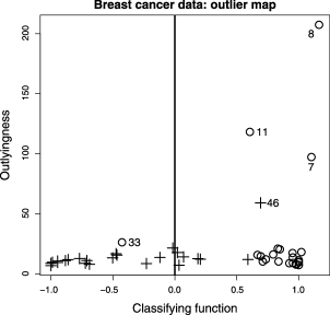
(a)

(b)

Figure 4: (a) Outlier map for the breast cancer data. Five outliers are clearly visible. Samples $7,8,11$ are outlying but well classified. Samples $33$ and $46$ are slightly outlying with respect to their groups, but are clearly wrongly classified. This suggests that they are mislabeled rather than erroneous, confirming the original analysis by West et al. (b) Same plot, but zoomed-in at the region $(0,30)$ on the vertical axis for better visibility. Observations flagged by algorithms searching for mislabelings are shown $(19,36,40,43,45,16)$.

Figure 5: Outlier map for the colon cancer data. Misclassifications and samples with large outlyingness are labeled. These were also flagged in the original analysis by Alon et al. (1999).

Figure 6: Outlier map for the protein data. The heterogeneity of the positive group is clearly visible, with different clusters according to the subgroups of different phyla, also confirming the original clustering analysis by Pollack et al. (2005).

5.3 Colon cancer data

The colon cancer data set from Alon et al. (1999) contains $2000$ gene expression levels for $40$ tumor samples and $22$ normal samples. The outlier map with a linear kernel is shown in Figure 5. In the tumor group T2, T33, T36 and T30 are misclassified. Sample T37 is classified correctly, but with low confidence: it is very close to the classification boundary. In the normal group N8 and especially N34 and N36 are the suspicious cases that behave differently from the other normal samples. The 8 aforementioned samples plus sample N12 were identified as possible outliers in the original paper by Alon et al. (1999) for biological reasons. Thus, 8 out of 9 true outliers can be identified on the outlier map, only leaving N12 undetected. However, in Malossini, Blanzieri and Ng (2006) none of the methods that were compared could detect N12. Moreover, the stability criterion proposed by Malossini et al. was unable to detect T37 and N8 too and incorrectly pointed at N2 and N28 as possibly suspicious samples. Also note the interesting sample T6. From the outlier map we see that this sample is classified correctly and with much confidence. Nevertheless, its outlyingness with respect to the other tumor samples is rather large. This means that T6 behaves quite differently than the other tumor samples, but without distorting the classification. In Malossini et al. most of the methods analyzed did not detect T6 at all. Again this is no surprise since methods such as the stability criterion of Malossini et al. specifically focus on mislabeled observations, whereas T6 is certainly not mislabeled. Only the outlier detection method of Kadota et al. (2003) is able to detect T6, but does rather poorly on the other samples detecting only 5 out of 9 true outliers.

5.4 Protein data

The protein data set taken from Pollack, Li and Pearl (2005) contains $131$ protein sequences of the essentially ubiquitous glycolytic enzyme 3-phosphoglycerate kinase (3-PGK) in three domains: Archaea, Bacteria and Eukaryota. The data set is available in the Protein Classification Benchmark Collection at http://net.icgeb.org (accession number PCB00015). We consider here classification task number 10 where the positive group consists of 35 Eukaryota. The negative group consists of 4 Archaea and 40 Bacteria. To classify these two groups of protein sequences, we use SVM with the local alignment kernel [Saigo et al. (2004)]. Default parameter values were used: gap opening penalty $=$ 11, gap extension penalty $=$ 1, scaling parameter $=$ 0.5. The outlier map is shown in Figure 6. One observes that the positive group of Eukaryota is very heterogeneous as several clusters appear. These clusters all have a biological interpretation, as the group of Eukaryota contains several subgroups of different phyla. For instance, observations 29–31 are from the phylum of Alveolata. Samples 13–17 are the Euglenozoa. Note that 18 (named Q8SRZ8), which belongs to the Fungi, was clustered in the group of Euglenozoa by Pollack et al.; this is actually confirmed by the outlier map. Finally, samples 33 and 34 are outlying with respect to the positive group. They form, together with 32, the group of Stramenopiles. Note that the different behavior of sample 32 from its fellow Stramenopiles is again a confirmation of the analysis by Pollack et al.: their clustering method assigned 32 (named Q8H721) in the main group of Eukaryota Metazoa. Also, in the outlier map 32 is situated in the main group, whereas 33 and 34 form a separate cluster. In the positive group the heterogeneity is less clear, although the 4 Archaea (36–39) do have the largest outlyingness compared to the other samples which are all Bacteria.

6 Conclusion

An outlier map is proposed for Support Vector Machine classification. If the outlier map shows two homogeneous and well classified groups, one can safely proceed analysis without worrying about outliers. However, in some situations this may not be the case and the outlier map can be a simple and useful tool to detect this. Moreover, the outlier map can be drawn for any choice of kernel, including rather exotic ones such as used in protein analysis. It can also be helpful to gain insight in the type of outliers, for example, whether outliers are mislabeled observations or not, or whether the outliers are isolated errors or rather a small subgroup of the group structure considered. This is important to know how to proceed analysis. If the outliers are truly erroneous observations, one should not take them into account to build a classifier, and one can manually discard them from the data set or apply a robust classifier. If the outliers are mislabeled observations, one probably should re-examine the labeling and change the label of the outlier if this seems indeed appropriate. If the outliers form a small subgroup of the data, one might reconsider the use of a binary classifier and turn to a more appropriate modeling technique. In any event, the outlier map can be helpful for practitioners of SVM classification to make such decisions.

References

- Alon et al. (1999) Alon, U., Barkai, N., Notterman, D. A., Gish, K., Ybarra, S., Mack, D. and Levine, A. J. (1999). Broad patterns of gene expression revealed by clustering of tumor and normal colon tissues probed by oligonucleotide arrays. Proc. Natl. Acad. Sci. 96 6475–6750.
- Chiaretti et al. (2004) Chiaretti, S., Li, X., Gentleman, R., Vitale, A., Vignetti, M., Mandelli, F., Ritz, J. and Foa, R. (2004). Gene expression profile of adult T-cell acute lymphocytic leukemia identifies distinct subsets of patients with different response to therapy and survival. Blood 103 2771–2778.
- Christmann and Steinwart (2004) Christmann, A. and Steinwart, I. (2004). On robustness properties of convex risk minimization methods for pattern recognition. J. Mach. Learn. Res. 5 1007–1034. \MR2248007
- Donoho (1982) Donoho, D. L. (1982). Breakdown properties of multivariate location estimators. Qualifying paper. Harvard Univ.
- Furey et al. (2000) Furey, T. S., Cristianini, N., Duffy, D., Bednarski, W., Schummer, M. and Haussler, D. (2000). Support vector machine classification and validation of cancer tissue samples using microarray expression data. Bioinformatics 16 906–914.
- Jaakkola, Diekhans and Haussler (2000) Jaakkola, T., Diekhans, M. and Haussler, D. (2000). A discriminative framework for detecting remote protein homologies. J. Comput. Biol. 7 95–114.
- Guyon et al. (2002) Guyon, I., Weston, J., Barnhill, S. and Vapnik, V. (2002). Gene selection for cancer classification using support vector machines. Mach. Learn. 46 389–422.
- Hubert and Engelen (2004) Hubert, M. and Engelen, S. (2004). Robust PCA and classification in biosciences. Bioinformatics 20 1728–1736.
- Hubert, Rousseeuw and Vanden Branden (2005) Hubert, M., Rousseeuw, P. J. and Vanden Branden, K. (2005). ROBPCA: A new approach to robust principal component analysis. Technometrics 47 64–79. \MR2135793
- Kadota et al. (2003) Kadota, K., Tominaga, D., Akiyama, Y. and Takahashi, K. (2003). Detecting outlying samples in microarray data: A critical assessment of the effect of outliers on sample classification. Chem-Bio. Inform. J. 3 30–45.
- Leslie, Ekin and Noble (2002) Leslie, C., Eskin, E. and Noble, W. S. (2002). The spectrum kernel: A string kernel for svm protein classification. In Proceedings of the Pacific Symposium on Biocomputing 2002 (R. B. Altman, A. K. Dunker, L. Hunter, K. Lauerdale and T. E. Klein, eds.) 564–575. World Scientific, Hackensack, NJ.
- Leslie et al. (2003) Leslie, C., Eskin, E., Weston, J. and Noble, W. S. (2003). Mismatch string kernels for svm protein classification. In Advances in Neural Information Processing Systems (S. Becker, S. Thrun and K. Obermayer, eds.) 15 1441–1448. MIT Press, Cambridge, MA.
- Li et al. (2001) Li, L., Darden, T. A., Weinberg, C. R., Levine, A. J. and Pedersen, L. G. (2001). Gene assessment and sample classification for gene expression data using a genetic algorithm/k-nearest neighbor method. Comb. Chem. High Throughput Screen. 4 727–739.
- Liao and Noble (2002) Liao, L. and Noble, W. S. (2002). Combining pairwise sequence similarity and support vector machines for remote protein homology detection. In Proceedings of the Sixth International Conference on Computational Molecular Biology (T. Lengauer, ed.) 225–232. ACM Press, New York.
- Malossini, Blanzieri and Ng (2006) Malossini, A., Blanzieri, E. and Ng, R. T. (2006). Detecting potential labeling errors in microarrays by data perturbation. Bioinformatics 22 2114–2121.
- Maronna and Yohai (1995) Maronna, R. and Yohai, V. (1995). The behavior of the Stahel–Donoho robust multivariate estimator. J. Amer. Statist. Assoc. 90 330–341. \MR1325140
- Pochet et al. (2004) Pochet, N., De Smet, F., Suykens, J. A. K. and De Moor, B. (2004). Systematic benchmarking of microarray data classification: Assessing the role of nonlinearity and dimensionality reduction. Bioinformatics 20 3185–3195.
- Pollack, Li and Pearl (2005) Pollack, J. D., Li, Q. and Pearl, D. K. (2005). Taxonomic utility of a phylogenetic analysis of phosphoglycerate kinase proteins of Archaea, Bacteria and Eukaryota: Insights by Bayesian analyses. Mol. Phylogenet. Evol. 35 420–430.
- Rousseeuw and Van Zomeren (1990) Rousseeuw, P. J. and Van Zomeren, B. C. (1990). Unmasking multivariate outliers and leverage points. J. Amer. Statist. Assoc. 85 633–639.
- Saigo et al. (2004) Saigo, H., Vert, J., Ueda, N. and Akutsul, T. (2004). Protein homology detection using string alignment kernels. Bioinformatics 20 1682–1689.
- Schölkopf and Smola (2002) Schölkopf, B. and Smola, A. (2002). Learning with Kernels. MIT Press, Cambridge, MA.
- Stahel (1981) Stahel, W. A. (1981). Robuste Schätzungen: Infinitesimale optimalität und schätzungen von kovarianzmatrizen. Ph.D. thesis, ETH Zürich.
- Steinwart and Christmann (2008) Steinwart, I. and Christmann, A. (2008). Support Vector Machines. Springer, New York. \MR2450103
- Vapnik (1998) Vapnik, V. (1998). Statistical Learning Theory. Wiley, New York. \MR1641250
- West et al. (2001) West, M., Blanchette, C., Dressman, H., Huang, E., Ishida, S., Spang, R., Zuzan, H., Marks, J. R. and Nevins, J. R. (2001). Predicting the clinical status of human breast cancer by using gene expression profiles. Proc. Natl. Acad. Sci. 98 11462–11467.