Hydrodynamic Interactions of Spherical Particles in A Fluid Confined by A Rough And No-Slip Wall

Abstract

In this article we develop a theoretical framework to study the hydrodynamic interactions in the presence of a non-flat and no-slip boundary. We calculate the influence of a small amplitude and sinusoidal deformations of a boundary wall in the self mobility and the two body hydrodynamic interactions for spherical particles. We show that the surface roughness enhances the self mobility of a sphere in a way that, for motion in front of a local hump of the surface, the mobility strength decreases while it increases for the motion above a local deep of the rough surface. The influence of the surface roughness in the two body hydrodynamic interactions is also analyzed numerically.

I Introduction

Hydrodynamic interaction of colloidal particles in confined geometries is an important problem in low Reynolds fluid dynamics happel . Fluid motions confined by one or two parallel flat planes are interesting examples with either analytical or numerical known solutions blake ; twoplate . The solution to these problems are involved in soft matter related phenomena and also microfluidic experiments micro ; microhyd ; zurita . In soft matter systems, swimming motion in a geometrically confined environment is a subject of growing interest lowen2 ; nanorod-wall ; raminconfined ; bacteriasurface , apparently better understanding of these systems requires a good knowledge of the hydrodynamic interactions in confined geometries. In microfluidic applications, a better control of the processes requires the prediction of the hydrodynamic effects due to the walls.

Confining wall can generate nontrivial effects. For example, in a very simple system composed of a single sphere near a wall, the mobility parallel to the wall is always larger than the perpendicular mobility happel which has been verified experimentally pralle ; dufresne . As other examples for the effects due to the boundaries, we address the experiments, showing that microorganisms, e.g. E. Coli chasb , bull spermatozoa chasb-ref6 , swimming in confined geometries are attracted by surfaces. In this article we concentrate on the effects due to the roughness of the confining walls. We will consider a rough wall that confines the fluid flow at low Reynolds number, and ask the following question, does the long wavelength roughness of the wall have any important influence on the one or two body hydrodynamic interactions? We use a perturbation method and investigate the case of a small amplitude and regular roughness on an infinite wall. We show that the roughness has important contributions in the hydrodynamic interactions.

Another challenging issue in the low Reynolds, quiescent fluid dynamics, is the validity of no-slip boundary condition. This is certainly important where the nano structure of the surface is involved. There are experimental and theoretical works, investigating the influence of the nano-roughness of the boundaries and justify the validity of the so-slip boundary conditions HS-noslip ; rough-boundary . Here we would like to stress the fact that, justification of the no-slip boundary condition, necessarily needs analytical results for rough surfaces taking into account the no-slip boundary condition.

The rest of this article is organized as follows: In Sec. II, we present a short review on Stokes flow and introduce the hydrodynamic interactions. Section III is devoted to the hydrodynamic effects of a rigid and flat wall. The effects of a general roughness is presented in sec. IV. An example of a sinusoidal roughness is considered in Sec. V. Concluding remarks are presented in sec. VI.

II Stokes flow and Hydrodynamic Interactions

To study the fluid motion for colloidal particles suspended in a fluid medium we define the Reynolds number as the ratio between the characteristic transport time scale due to diffusion and the convection time over a length $L$. Denoting the fluid density by $\rho$, viscosity by $\eta$, typical velocity by $U$ and also the linear size of the particles by $a$, we see that the Reynolds number is $Re=\frac{Ua\rho}{\eta}$. In a wide variety of phenomena occurring in the motion of micron scale particles, the Reynolds number is very low. For these phenomena we can consider the limit of zero Reynolds number. At zero Reynolds number the fluid dynamics is expressed by Stokes equation. Denoting the fluid velocity and pressure fields by ${\bf u}({\bf x})$ and $P({\bf x})$, the Stokes and continuity equations for an incompressible flow can be written as:

$$\eta\nabla^{2}{\bf u}({\bf x})-\nabla P({\bf x})={\bf f}^{ext},~{}~{}\nabla\cdot{\bf u}({\bf x})=0,$$ (1)

where ${\bf f}^{ext}$, denotes the density of external body force acting on the fluid. The fluid velocity field is subject to no-slip boundary condition on the surface of solid boundaries. We would like to consider the motion of $N$ colloidal particles suspended is a low Reynolds flow (see Fig. 1). Recalling the fact that the governing equations are linear with respect to the velocity profile, and applying the no-slip boundary condition on the surface of rigid particles, we can eliminate the fluid velocity and obtain a set of linear equations relating the particle velocities to the hydrodynamic forces acting on them. Denoting the velocity of $m$’th particle by ${\bf v}^{m}$ and the corresponding hydrodynamic force by ${\bf f}^{m}$, we can write the following equation:

$${\bf v}_{i}^{m}=\sum_{n=1}^{N}\sum_{j=1}^{3}D_{ij}^{mn}\times{\bf f}_{j}^{n}.$$ (2)

Coefficients $D_{ij}^{mn}$ are know as the elements of hydrodynamic interaction. Quite similar to the Onsager relations in thermodynamics and based on general symmetry arguments and microscopic reversibility, the hydrodynamic tensor $D_{ij}^{mn}$ is symmetric with respect to its up or down indices reichel ; dhont . For special case of $2$ particles (denoted by $\alpha$ and $\beta$), and for convenience we define the self mobility tensor as the response of a particle to the force acting on it by $\mu_{ij}=D_{ij}^{\alpha\alpha}$. And also the hydrodynamic response of $\alpha$’th particle to the force acting on $\beta$’th particle is shown by: $M_{ij}=D_{ij}^{\alpha\beta}=D_{ij}^{\beta\alpha}$. Different components of the hydrodynamic interaction tensor depend on the size and the relative configurations of the particles.

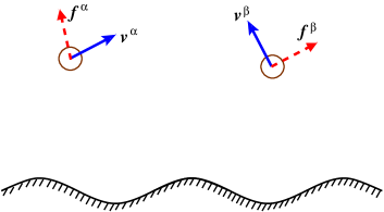
Figure 1: (color online). Two spherical particle is moving in a low Reynolds flow. The fluid flow is bounded by a rough, rigid and no-slip boundary. Velocities and hydrodynamic forces acting on particles are shown in this picture.

Calculating the hydrodynamic interaction tensor, is an important problems in low Reynolds hydrodynamics. Here we present an analytic method that is useful for very small and spherical particles. A very small sphere can be considered as a point force, a source term in the Stokes equation. Denoting the point force by ${\bf f}({\bf x})={\bf b}~{}\delta({\bf x}-{\bf x}_{0})$, the velocity field of the point force, can be written as Oseen ; pozrikidis :

$${\bf u}_{i}({\bf x})=\sum_{j=1}^{3}{G_{ij}}({\bf x},{\bf x}_{0})\times{\bf b}_{j},$$ (3)

and correspondingly the associated pressure field is given by: $P({\bf x})={\bf\Pi}({\bf x},{\bf x}_{0})\cdot{\bf b}$. Here $G_{ij}({\bf x},{\bf x}_{0})$ is the Green’s function of the Stokes differential equation.

Solving the Stokes equations and having the associated Green’s function for any required geometry, we can use Faxén’s theorem for spherical objects with radius $a$ to express the mobility tensor in terms of the Green’s function of Stokes equation happel ; Kim :

$$D_{ij}^{\alpha\beta}({\bf x}^{\alpha},{\bf x}^{\beta})=(1+\frac{a^{2}}{6}\nabla^{2}_{{\bf x}^{\alpha}})(1+\frac{a^{2}}{6}\nabla^{2}_{{\bf x}^{\beta}})G_{ij}({\bf x}^{\alpha},{\bf x}^{\beta}).$$ (4)

For very small spheres with radius $a$ smaller than the typical distance between spheres, then $D_{ij}^{\alpha\beta}({\bf x}^{\alpha},{\bf x}^{\beta})=G_{ij}^{F}({\bf x}^{\alpha},{\bf x}^{\beta})$ up to second order in $a$ infinite .

In the rest of this article, we use the above method and presents the results for unconfined ($U$), confined with a flat wall ($F$) and confined with a rough wall ($R$). The effects due to roughness is considered for a very small amplitude roughness.

III Hydrodynamics Near a Flat and No-Slip Wall

We first consider the case of a fluid flow that is bounded by a rigid, flat ($F$) and no-slip plane located at $z=0$. The solution to the problem of a point force in the presence of a flat wall is given by Blake blake ; pozrikidis , who has used the image method to construct the solutions. The flat wall Green’s function for the upper half space ($z>0$), is given by:

$$G_{ij}^{F}({\bf x},{\bf x}_{0}) = G_{ij}^{U}({\bf x},{\bf x}_{0})-G_{ij}^{U}({\bf x},{\bf x}^{im}_{0})$$ (5)

$$+ G_{ij}^{D}({\bf x},{\bf x}^{im}_{0})-G_{ij}^{SD}({\bf x},{\bf x}_{0}^{im}),$$

where the Green’s function for an unbounded ($U$) fluid flow $G_{ij}^{U}$, that is called stokeslet is given by:

$$G_{ij}^{U}({\bf x},{\bf x}_{0})=\frac{1}{8\pi\eta}\left(\frac{\delta_{ij}}{r}+\frac{r_{i}r_{j}}{r^{3}}\right),$$ (6)

here ${\bf r}={\bf x}-{\bf x}_{0}$, and ${\bf x}^{im}_{0}={\bf x}_{0}-2\left({\hat{z}}\cdot{\bf x}_{0}\right){\hat{z}}$ is the image position of the point force with respect to the flat wall. Defining a new vector ${\bf R}={\bf x}-{\bf x}^{im}_{0}$, we can express the potential dipole field $G_{ij}^{D}$, and stokeslet dipole $G_{ij}^{SD}$ as:

$$G_{ij}^{D}({\bf x},{\bf x}^{im}_{0})=\frac{2}{8\pi\eta}z_{0}^{2}(1-2\delta_{jz})\frac{\partial}{\partial R_{j}}\left(\frac{R_{i}}{R^{3}}\right),$$ (7)

$$G_{ij}^{SD}({\bf x},{\bf x}^{im}_{0})=2z_{0}(1-2\delta_{jz})\frac{\partial}{\partial R_{j}}G_{iz}^{U}({\bf x},{\bf x}^{im}_{0}),$$ (8)

where $z={\hat{z}}.{\bf x}$. The pressure field for the flow that is bounded by a flat wall is given by:

$${\bf\Pi}^{F}({\bf x},{\bf x}_{0}) = {\bf\Pi}^{U}({\bf x},{\bf x}_{0})+{\bf\Pi}^{U}({\bf x},{\bf x}^{im}_{0})$$ (9)

$$- 2z_{0}\frac{\partial}{\partial{\bf R}}\left({\hat{z}}\cdot{\bf\Pi}^{U}({\bf x},{\bf x}^{im}_{0})\right),$$

where the pressure field associated to a point force in an unbounded space is given by:

$${\bf\Pi}^{U}({\bf x},{\bf x}_{0})=\frac{2}{8\pi}~{}\frac{\left({\bf x}-{\bf x}_{0}\right)}{|{\bf x}-{\bf x}_{0}|^{3}},$$ (10)

Having in hand all the above information, we can calculate the hydrodynamic interactions in the presence of a flat no-slip wall.

As an example and using the above formalism we present the results for the self mobility of a very small sphere moving above a flat and no-slip wall. Denoting the perpendicular distance between the sphere and wall by $H$, and assuming that $H$ is greater than the sphere radius $a$, the components of self mobility tensor are happel ; Kim

$$\mu^{F}_{xx} = \mu_{0}(1-\frac{9}{16}\frac{a}{H}+{\cal O}(\frac{a}{H})^{2}),$$

$$\mu^{F}_{zz} = \mu_{0}(1-\frac{9}{8}\frac{a}{H}+{\cal O}(\frac{a}{H})^{2}),$$ (11)

where $\mu_{0}={1}/{(6\pi\eta a)}$ is the self mobility of a spherical particle moving in an unbounded fluid. As an important and non-trivial result, the above equations show that, the self mobility of the sphere in the direction parallel to the wall is always larger than the perpendicular direction happel . This effect has been verified experimentally pralle . Calculations show that, up to ${\cal O}(\frac{a}{H})^{2}$, other components of the self mobility tensor are zero.

IV Effects Due to a Rough and No-Slip Wall

The aim of this article is to express analytical expressions for hydrodynamic interactions in a semi infinite flow, bounded by a rough ($R$), rigid and no-slip wall. Fig. 1 shows the schematic view of a rough plane that bounds the fluid flow. Two spherical particles located at positions ${\bf x}^{\alpha}$ and ${\bf x}^{\beta}$ are moving in the fluid. The position vector for the points on the bounding wall is considered as: ${\bf x}_{s}=(x,y,h(x,y))$. This kind of parametrization allows us to obtain the results of a flat wall by considering the limiting case of $h(x,y)=0$. For later use we define ${\bf x}^{0}_{s}=(x,y,0)$, that is denoting the location of the points of a flat wall located at $z=0$.

Applying the no-slip boundary condition on the rough surface ($R$), we expect that the influence of the roughness will produce non-trivial effects. To study the hydrodynamic effects of a rigid and rough wall with small amplitude roughness, we can construct a perturbation expansion. Introducing a small dimensionless parameter $\varepsilon={h_{0}}/{z}$, where $h_{0}$ is the typical amplitude for height fluctuations and $z$ measures the distance of particles from the wall, we expand all quantities in powers of $\varepsilon$. As explained before, hydrodynamic interaction between small spherical particles can be obtained by solving the velocity field of a point force for the required geometry. Here the solutions to the Stokes-Green’s equation should be obtained by applying the required boundary condition. The velocity field of a point force satisfies the Stokes equation (Eq. 1) and is subject to to the following boundary condition:

$${\bf u}({\bf x}_{s})=0.$$ (12)

Expanding the corresponding velocity and pressure field of a point force in the presence of a rough wall in powers of $\varepsilon$, we can write:

$${\bf u}^{R}({\bf x}) = {\bf u}^{(0)}({\bf x})+{\bf u}^{(1)}({\bf x})+{\bf u}^{(2)}({\bf x})+{\cal O}(\varepsilon^{3}),$$

$$P^{R}({\bf x}) = P^{(0)}({\bf x})+P^{(1)}({\bf x})+P^{(2)}({\bf x})+{\cal O}(\varepsilon^{3}),$$ (13)

The zeroth order term are the velocity and pressure field of point force in the presence of a flat($F$) and no-slip wall. In this case we will have:

$${\bf u}^{(0)}({\bf x})={\bf u}^{F}({\bf x}),~{}~{}{\bf P}^{(0)}({\bf x})={\bf P}^{F}({\bf x}).$$ (14)

Higher order corrections due to the wall roughness, can be obtained by noting that different order of the velocity and pressure fields are satisfied the following differential equation:

$$\eta\nabla^{2}{\bf u}^{(n)}({\bf x})-\nabla P^{(n)}({\bf x})=0,~{}~{}\nabla\cdot{\bf u}^{(n)}({\bf x})=0,$$ (15)

where the boundary conditions for the first and second orders are given explicitly by:

$${\bf u}^{(1)}({\bf x}_{s}^{0}) = -h({\bf x}_{s}^{0})\frac{\partial{\bf u}^{(0)}({\bf x}_{s}^{0})}{\partial z}.$$

$${\bf u}^{(2)}({\bf x}_{s}^{0}) = -h({\bf x}_{s}^{0})\frac{\partial{\bf u}^{(1)}({\bf x}_{s}^{0})}{\partial z}-\frac{h^{2}({\bf x}_{s}^{0})}{2}\frac{\partial^{2}{\bf u}^{(0)}({\bf x}_{s}^{0})}{\partial^{2}z}.$$

As one can see the velocity field at order $(n)$, is related to the local value of the derivatives of the velocity filed at order of $(n-1)$, in the position of flat wall. Using the well known integral representation for the flow field of Stokes equation, we can write the following integral solution pozrikidis :

$${\bf u}_{j}^{(n)}({\bf x})=\frac{1}{8\pi}\int{\bf u}_{i}^{(n)}({\bf x^{\prime}}){\bf T}_{ijk}({\bf x,x^{\prime}})dS_{k}({\bf x^{\prime}}),$$ (17)

where the integration is carried out on a closed surface composed of an infinite plane at $z=0$. The surface is closed at the upper half space and $d{\bf S}({\bf x}^{\prime})$ is the area element on this surface in the inward direction (here is ${\hat{z}}$). The stress tensor ${\bf T}_{ijk}({\bf x},{\bf x}^{\prime})$ is given by:

$${\bf T}_{ijk}({\bf x},{\bf x}^{\prime}) = -8\pi\delta_{ik}\Pi^{F}_{j}({\bf x},{\bf x}^{\prime})+8\pi\eta\frac{\partial}{\partial x_{k}}G^{F}_{ij}({\bf x},{\bf x}^{\prime})$$ (18)

$$+ 8\pi\eta\frac{\partial}{\partial x_{i}}G^{F}_{kj}({\bf x},{\bf x}^{\prime}).$$

Now we can expand the hydrodynamic interaction tensor moving in a fluid bounded by a rough wall, in terms of small parameter $\varepsilon$ as:

$${\bf D}^{R}={\bf D}^{(0)}+{\bf D}^{(1)}+{\bf D}^{(2)}+{\cal O}(\varepsilon^{3}),$$ (19)

where the zeroth order is the results of a sphere moving in a medium bounded by a flat ($F$) and no-slip wall:

$$D^{(0)}_{ij}=D^{F}_{ij}\approx G_{ij}^{F}.$$ (20)

Using Eqs. (3), (4), (17) and considering the explicit form of the stress tensor ${\bf T}_{ijk}({\bf x}_{\beta},{\bf x}_{0}^{s})$, we can arrive at the following expressions for the first and second order corrections to the mobility tensor due to the roughness of the wall:

$$8\pi\eta\times D^{(1)}({\bf x}_{\alpha},{\bf x}_{\beta}) = -\frac{1}{8\pi}\int D^{\prime(0)}({\bf x}_{\alpha},{\bf x}_{s}^{0})D^{\prime(0)}({\bf x}_{\beta},{\bf x}_{s}^{0})h({\bf x}_{s}^{0})d^{2}{\bf x}_{s}^{0},$$ (21)

$$256\pi^{2}\eta\times D^{(2)}({\bf x}_{\alpha},{\bf x}_{\beta}) = \frac{1}{2\pi}\int\int D^{\prime(0)}({\bf x}_{\alpha},{\bf x}_{s}^{0})D^{\prime(0)}({\bf x}_{\beta},{\bf x^{\prime}}_{s}^{0})D^{\prime\prime(0)}({\bf x}_{s}^{0},{\bf x^{\prime}}_{s}^{0})h({\bf x}_{s}^{0})h({\bf x^{\prime}}_{s}^{0})d^{2}{\bf x}_{s}^{0}d^{2}{\bf x^{\prime}}_{s}^{0}$$

$$-\int\Big{(}E^{(0)}({\bf x}_{\alpha},{\bf x}_{s}^{0}){\ddot{D}}^{(0)}({\bf x}_{\beta},{\bf x}_{s}^{0})~{}+~{}(\alpha\leftrightarrow\beta)\Big{)}h^{2}({\bf x}_{s}^{0})d^{2}{\bf x}_{s}^{0},$$

where

$$D^{\prime(0)}({\bf x}_{\beta},{\bf x}_{s}^{0}) = \frac{\partial}{\partial z}D^{(0)}({\bf x}_{\beta},{\bf x})\mid_{{\bf x}\rightarrow{\bf x}_{s}^{0}}$$

$$D^{\prime\prime(0)}({\bf x}_{s}^{0},{\bf x^{\prime}}_{s}^{0}) = \frac{\partial^{2}}{\partial z\partial z^{\prime}}D^{(0)}({\bf x},{\bf x^{\prime}})\mid_{({\bf x},{\bf x^{\prime}})\rightarrow({\bf x}_{s}^{0},{\bf x^{\prime}}_{s}^{0})}$$

$${\ddot{D}}^{(0)}({\bf x}_{\beta},{\bf x}_{s}^{0}) = \frac{\partial^{2}}{\partial z^{2}}D^{(0)}({\bf x}_{\beta},{\bf x})\mid_{{\bf x}\rightarrow{\bf x}_{s}^{0}},$$ (23)

and $E^{(0)}_{ij}=\Pi^{(F)}_{ij}\delta_{i=z}+D^{\prime(0)}_{ij}\delta_{i\neq z}$. As one can see, the mobility tensor is symmetric: $D({\bf x}_{\alpha},{\bf x}_{\beta})=D({\bf x}_{\beta},{\bf x}_{\alpha})$.

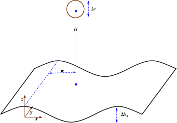
Figure 2: (color online). A spherical particle is moving in a confined fluid flow. The roughness of the boundary is assumed to be a sinusoidal pattern with wavelength $\lambda$ in the $x$ direction. The boundary is assumed to be invariant under translation along the $y$ direction. Two parameters, $H$ the average vertical distance from the wall, and $w$ the vertical deviation from a local hump of the surface roughness, characterize the sphere’s position.

In the following section we choose a very special form of the wall deformation pattern and investigate the hydrodynamic interactions.

V Sinusoidal Roughness

As a special example we assume that the wall roughness is a sinusoidal deformations of a flat wall located at $z=0$. The height profile of the rough plane, in the Monge representation, is given by the following equation:

$$z=h(x,y)=h_{0}\cos(qx+\phi),$$ (24)

where $h_{0}$ is the amplitude of the roughness, and the wave vector of the roughness along the $x$ axis is denoted by $q$. This special type of roughness allows us to study any general roughness that is invariant under translation along $y$ direction.

As a special feature of the hydrodynamic interaction we concentrate on the self mobility of a spherical particle moving in a medium bounded by a rough and no-slip wall. Fig. 2, shows the schematic view of a sphere with size $a$, moving near a rough wall. Perpendicular projection of the sphere position into the $z=0$ plane, is deviated from the wall hump by a distance $w$. Denoting the wave length of the wall roughness by $\lambda=\frac{2\pi}{q}$, and the average height of the particle on the wall by $H$, we define a dimensionless parameter by $\gamma=2\pi\frac{H}{\lambda}$. Now following the method developed in the preceding sections, the first order corrections to the different components of the self mobility are given by:

$$\mu_{xx}^{(1)} = \frac{1}{8\pi\eta H}\frac{h_{0}}{H}\cos(\phi)\Big{[}-\frac{9}{32}\gamma^{2}K_{2}(\gamma)$$

$$+36\gamma^{2}\int_{0}^{\infty}\frac{s^{5}J_{2}(s)}{(s^{2}+\gamma^{2})^{5}}ds\Big{]},$$

$$\mu_{yy}^{(1)} = \frac{1}{8\pi\eta H}\frac{h_{0}}{H}\cos(\phi)\Big{[}-\frac{9}{32}\gamma^{2}K_{2}(\gamma)\Big{]},$$

$$\mu_{zz}^{(1)} = 0,$$

and the second order corrections are given by:

$$\mu_{xx}^{(2)} = \frac{1}{8\pi\eta H}\frac{h_{0}^{2}}{H^{2}}\Big{\{}\frac{3}{32}+\cos(2\phi)\Big{[}\frac{15}{32}\gamma^{3}K_{3}(2\gamma)$$

$$-\frac{9}{8}\gamma^{4}K_{0}(2\gamma)+\frac{3}{8}\gamma^{5}K_{1}(2\gamma)$$

$$-\frac{9}{8}\gamma^{3}K_{1}(2\gamma)-9\gamma^{6}\int_{0}^{\infty}\frac{s^{3}J_{0}(2s)}{(s^{2}+\gamma^{2})^{5}}ds\Big{]}$$

$$+36\cos^{2}(\phi)e^{-\gamma}(1-\gamma)\Big{[}I_{2}(\gamma/2)K_{2}(\gamma/2)$$

$$-\gamma^{4}\int_{0}^{\infty}\frac{J_{2}(s)}{(s^{2}+\gamma^{2})^{5/2}}ds\Big{]}\Big{\}},$$

$$\mu_{yy}^{(2)} = \frac{1}{8\pi\eta H}\frac{h_{0}^{2}}{H^{2}}\Big{\{}\frac{3}{32}+\frac{15}{32}\cos(2\phi)\gamma^{3}K_{3}(2\gamma)$$

$$+36\cos^{2}(\phi)e^{-\gamma}I_{2}(\gamma/2)K_{2}(\gamma/2)\Big{\}},$$

$$\mu_{zz}^{(2)} = \frac{1}{8\pi\eta H}\frac{h_{0}^{2}}{H^{2}}\Big{\{}\frac{9}{8}+\frac{9}{8}\cos(2\phi)\Big{[}-\gamma^{4}K_{4}(2\gamma)$$ (26)

$$+\frac{1}{3}\gamma^{5}K_{5}(2\gamma)\Big{]}\Big{\}},$$

Where $\phi=\frac{2\pi}{\lambda}w$ measures the deviation of the perpendicular projection of the sphere from a local hump on the surface. Here $J_{n}(\gamma)$ , $I_{n}(\gamma)$ and $K_{n}(\gamma)$ are Bessel’s function of the order $n$ GradRyzh .

We can investigate the effects of the roughness in two extreme limits of long or short wavelength deformations. For the case of very short wave length deformations, $\lambda\ll H$ ($\gamma\gg 1$) one can see that the roughness has no net effects on the self mobility of a spherical particle moving very far from the wall (up to first order of $\varepsilon$). In this case the mobility tensor is effectively given by the mobility tensor of a sphere located very far from a flat wall. The explicit form of the mobility tensor for this case is given by Eq. (11). The back flows, scattered from the humps and deeps of the wall have cancelled out the effects of each other and the overall averaged back flow looks like a back flow from a flat wall.

In the case of a very long wavelength roughness where $\lambda\gg H$ ($\gamma\ll 1$), we proceed and obtain the second order corrections (in terms of $\varepsilon$) to the self mobility components. Now we can expand this result around small $\gamma$, to reach the following expressions for the different elements of the self mobility tensor:

$$\mu_{xx}^{R} \approx \mu_{xx}^{F}+\mu_{0}\frac{9}{4}(\frac{ah_{0}^{2}}{H^{3}})\Big{[}\frac{1}{32}(1+5\cos(2\phi))$$

$$+3\cos^{2}(\phi)\Big{]},$$

$$\mu_{yy}^{R} \approx \mu_{yy}^{F}-\mu_{0}\Big{[}\frac{27}{64}(\frac{ah_{0}}{H^{2}})\cos(\phi)$$

$$-\frac{9}{4}(\frac{ah_{0}^{2}}{H^{3}})\left(\frac{1}{32}(1+5\cos(2\phi))+3\cos^{2}(\phi)\right)\Big{]},$$

$$\mu_{zz}^{R} \approx \mu_{zz}^{F}+\mu_{0}\frac{27}{32}(\frac{ah_{0}^{2}}{H^{3}})(1+\cos(2\phi)).$$ (27)

As one can see, the effects due to the roughness, enhances the self mobility tensor of a sphere in asymmetric way with respect to the in plane ($x$ and $y$) directions. We define the asymmetric parameter as the difference between the mobilities in the $x$ and $y$ directions:

$$\Delta\mu=\mu_{xx}^{R}-\mu_{yy}^{R}=\mu_{0}\left[\frac{27}{64}(\frac{ah_{0}}{H^{2}})\cos(\phi)\right].$$ (28)

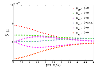
Figure 3: (color online). Different components of self mobility tensor $\delta\mu_{ii}=(\mu^{R}_{ii}-\mu^{F}_{ii})/\mu_{ii}^{F}$ for a spherical particle moving adjacent to a non-smooth and no-slip wall are plotted as a functions of the particle’s separation from the wall. Here the wave vector for surface roughness lies along the $x$ direction. All three components of the self mobility tensor are plotted for two special cases of motion above a hump or deep of the surface deformations. As one can see for $\phi=0$ (sphere move over a local hump), the roughness decreases the parallel components of self mobility while for $\phi=\pi$ (motion over a local deep), they increase. Parameter values for these graphs are: $h_{0}/H=0.1$, $a/H=0.1$.

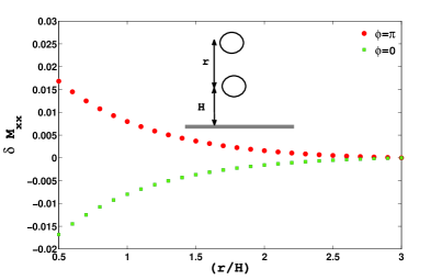
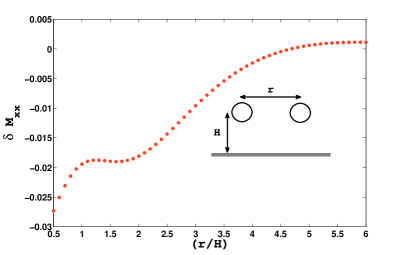
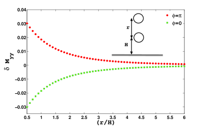
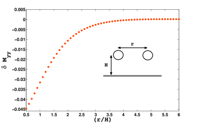
Figure 4: (color online). Different components of the hydrodynamic interaction tensor $\delta M_{ii}=8\pi\eta H(M^{R}_{ii}-M^{F}_{ii})$, for two spherical particles moving parallel to the wall, are plotted as a functions of the particle’s separation. Here the wave vector for surface roughness lies along the $x$ direction. At right graphs (up and down), the interaction is plotted for the case where the position of the first sphere is fixed at $\phi=0$ and we changed the position of the second sphere. There is a periodicity with the wavelength of the roughness. As one can see in the case of left graphs, for $\phi=0$ (sphere move over a local hump), the roughness decreases the interaction strength while for $\phi=\pi$ (motion over a local deep), it increases. Parameter values for these graphs are: $\lambda/H=10$, $h_{0}/H=0.1$, $a/H=0.1$.

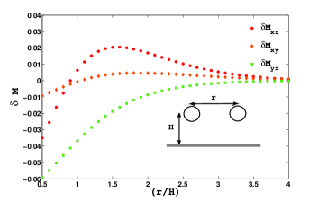
Figure 5: (color online). Off diagonal components of the hydrodynamic interaction tensor $\delta M_{ij}=8\pi\eta H(M^{R}_{ij}-M^{F}_{ij})$, for two spherical particles, are plotted as a functions of the particle’s separation. Here the wave vector for surface roughness lies along the $x$ direction. Parameter values for these graphs are: $\lambda/H=10$, $h_{0}/H=0.1$, $a/H=0.1$.

The sign of the asymmetric parameter depends on the local position of the sphere. In terms of the back flow scattered from the wall and in the limit of long wave length deformations, it is expected that the nearest hump or deep will have the dominant contributions on the particle motion. Over a local hump ($0<\phi<\pi/2$), $\mu_{xx}^{R}>\mu_{yy}^{R}$, while over a local deep ($\pi/2<\phi<3\pi/2$), $\mu_{xx}^{R}<\mu_{yy}^{R}$. Interestingly for a special points of $\phi=\pi/2,3\pi/2$, the mobility tensor is symmetric.

To analyze the self mobility for intermediate $\gamma$ ($H\sim\lambda$), we have presented numerical plots in Fig. 3. As one can see for $H\sim\lambda$, the change in the mobility of a sphere mediated by roughness changes its sign for motion above a peak or above a valley.

To demonstrate the effects of roughness on the two-body interactions, we have presented in Fig. 4 and Fig. 5, numerical results for diagonal and off diagonal elements of hydrodynamic interactions. In these examples we have studied the hydrodynamic interactions for some different cases. In Fig. 4 we have plotted $M_{xx}(r)$ (up) and $M_{yy}(r)$ (down). In Fig. 4, right part (up and down), we have plotted the interactions of two spheres that have same vertical distance $H$ from the wall. As one can see, the roughness always decreases the strength of $M_{xx}(r)$ and $M_{yy}(r)$. There is a very weak periodicity with the wavelength of the roughness. In the left part of Fig. 4 (up and down), we have plotted the hydrodynamic interaction as a function of vertical separation of two spherical particles. The results for this case, depend on the local position of the spheres with respect to the surface roughness. As one can see for $\phi=0$ (spheres move over a local hump), the roughness decrease the interaction strength while for $\phi=\pi$ (motion over a local deep), it increases. As another example, some of off diagonal components of the two body hydrodynamic interactions are plotted in Fig. 5. There is a very weak periodicity with wavelength $\lambda$, that is not clearly seen in the scale of this graph.

VI concluding remarks

In this article we have considered the influence of a rough, rigid and no-slip boundary wall on the hydrodynamic interactions of spherical particles. We have studied a regular sinusoidal roughness pattern with very small amplitude roughness on a flat plane. For simplicity we have studied a simple wave with a single wave vector along $x$ direction. Taking into account the wall effects by applying the no-slip boundary condition by standard perturbation technique, we have calculated one and two-body hydrodynamic effects. For a single and small radius sphere moving in the presence of a rough wall, we show that, the different elements of self mobility tensor changes in asymmetric way. Motion along the wave vector of surface roughness is different from the other in-plane direction. When a spherical colloid suspended near a rough and no-slip wall, the hydrodynamic drag force depends on the local position of the sphere. Roughness will produce different contributions for motion on a local hump or a local deep of the wall. This kind of behavior in two-body hydrodynamic interaction is also seen by numerical investigations of different components of the hydrodynamic interactions.

We note that in the current formulation of the problem, we have made some approximations which need to be dealt with carefully. Caution is needed in applying the results since there are many length scales in the problem: $a$, $h_{0}$, $\lambda$ and $H$. First, the Faxen’s formula has allowed us to treat the sphere’s size in a series expansion in powers of $\epsilon_{1}=(a/H)$. Second approximation is related to the slowly varying roughness of the wall and consequently to a series expansion of the results in powers of $\epsilon_{2}=(h_{0}/H)$. The series expansion for a typical component of the hydrodynamic interactions, for example the self mobility, have the following structure:

$$\Delta\mu/\mu_{0}=\epsilon_{1}\times \Big{\{} \left[f_{11}(\gamma)\epsilon_{2}+f_{12}(\gamma)\epsilon_{2}^{2}+{\cal O}(\epsilon_{2}^{3})\right]$$ (29)

$$+ \left[f_{21}(\gamma)\epsilon_{2}+f_{22}(\gamma)\epsilon_{2}^{2}+{\cal O}(\epsilon_{2}^{3})\right]\epsilon_{1}$$

$$+ {\cal O}(\epsilon_{1}^{2})\Big{\}},$$

where we have already defined $\gamma=2\pi(H/\lambda)$. The results are valid for any $\gamma$, however one should note that, the convergence of the above series expansion in the limit of very small $\gamma$ ($\gamma\ll 1$), is constrained to the condition $(h_{0}/\lambda)\ll 1$. By small roughness assumption, one expects that this criterion is satisfied as well.

In conclusion, we have developed a systematic way to evaluate the perturbation effects of a rough wall in the hydrodynamical properties of small spherical particles. The results of current work can be used in many directions related to the colloidal problems in confined flows, where the roughness is an ignorable characteristics of most walls. The influence of wall roughness on the thermal diffusion of colloidal particles is an interesting issue that we are considering. Inspired by the ensemble of low Reynolds swimmers, we are also investigating the motion of low Reynolds self propellers adjacent to a rough wall.

- (1) J. Happel and H. Brenner, Low Reynolds Number Hydrodynamics, (Noordhoff, Leyden, 1973).
- (2) N. Liron and S. Mochon, Journal of Engineering Math. 10, 287 (1976); M.E. Staben et al., Physics of Fluid 15, 1711 (2003); B. Lin et al., Phys. Rev. E 62, 3909 (2000).
- (3) J.R. Blake, Proc. Cambridge Philos. Soc. 70, 303 (1971).
- (4) P. Tabeling, Introduction to Microfluidics, (Oxford university press, Oxford, 2005).
- (5) S. Kim and S. J. Karrila, Microhydrodynamics: Principles and Selected Applications, (Dover Publications, 1991).
- (6) M. Zurita-Gotori, J. Blawzdziewiczi and E. Wajnryb, J. Fluid Mech. 592, 447 (2007).
- (7) H.H. Wensink and H. Löwen, Phys. Rev. E 78, 031409 (2008); S. van Teeffelen and H. Löwen, ibid. 78, 020101(R) (2008).
- (8) C. Sendner and R.R. Netz, Europhys. Lett. 79, 58004 (2007).
- (9) P. Tierno, R. Golestanian, I. Pagonabarraga, and F. Sagu s, Phys. Rev. Lett. 101, 218304 (2008).
- (10) P.D. Frymier, R.M. Ford, H.C. Berg, and P.T Cummings, Proc. Natl. Acad. Sci. 92, 6195 (1995).
- (11) A. Pralle et al., Appl. Phys. A 66, S71 (1998).
- (12) E.R. Dufresne, T.M. Squires, M.P. Brenner, and D.G. Grier, Phys. Rev. Lett. 85, 3317 (2000).
- (13) A.P. Berke, L. Turner, H.C. Berg, and E. Lauga, Phys. Rev. Lett. 101 , 038102 (2008).
- (14) L. Rothschild, Nature (London) 198, 1221 (1963).
- (15) E. Lauga, M.P. Brenner and Howard A. Stone, Microfluidics: The no-slip boundary condition, Chapter 19 in: Handbook of Experimental Fluid Dynamics,(Springer, 2007).
- (16) O.I. Vinogradova and G.E. Yakubov, Phys. Rev E 73, 045302(R) (2006); E. Bonaccurso et al., Phys. Rev. Lett. 90, 144501-1 (2003); Y. Zhu and S. Granick, Phys. Rev. Lett. 88, 106102-1 (2002).
- (17) L.E. Reichl, A Modern Course in Statistical Physics, (John Wiley and Sons Inc., New York, 1998).
- (18) J.K.G. Dhont, An Introduction to Dynamics of Colloids, (Elsevier Science B. V., 2003).
- (19) C. Pozrikidis, Boundary Integral and Singularity Methods for Linearized Viscous Flow, (Cambridge university ress, New York, 1992).
- (20) C.W. Oseen, Neuere Methoden und Ergebniss in der Hydrodynamik, (Akademishe Verlagsgesellschaft. 1927).
- (21) Y.W. Kim and R.R. Netz, J. Chem. Phys. 124, 114709, (2006).
- (22) As a simple prescription for regularization, in calculating the components of self mobility, we replace all divergent terms with the self mobility of a sphere , that is also divergent for a very small sphere.
- (23) I.S. Gradshteyn and I.M. Ryzhik, Table of Integrals, Series, and Products, (Academic Press, United Kingdom, London, 1965).