Molecular Distributions in Gene Regulatory Dynamics

Abstract

We show how one may analytically compute the stationary density of the distribution of molecular constituents in populations of cells in the presence of noise arising from either bursting transcription or translation, or noise in degradation rates arising from low numbers of molecules. We have compared our results with an analysis of the same model systems (either inducible or repressible operons) in the absence of any stochastic effects, and shown the correspondence between behaviour in the deterministic system and the stochastic analogs. We have identified key dimensionless parameters that control the appearance of one or two steady states in the deterministic case, or unimodal and bimodal densities in the stochastic systems, and detailed the analytic requirements for the occurrence of different behaviours. This approach provides, in some situations, an alternative to computationally intensive stochastic simulations. Our results indicate that, within the context of the simple models we have examined, bursting and degradation noise cannot be distinguished analytically when present alone.

1 Introduction

In neurobiology, when it became clear that some of the fluctuations seen in whole nerve recording, and later in single cell recordings, were not simply measurement noise but actual fluctuations in the system being studied, researchers very quickly started wondering to what extent these fluctuations actually played a role in the operation of the nervous system.

Much the same pattern of development has occurred in cellular and molecular biology as experimental techniques have allowed investigators to probe temporal behaviour at ever finer levels, even to the level of individual molecules. Experimentalists and theoreticians alike who are interested in the regulation of gene networks are increasingly focussed on trying to access the role of various types of fluctuations on the operation and fidelity of both simple and complex gene regulatory systems. Recent reviews (Kaern et al., 2005; Raj and van Oudenaarden, 2008; Shahrezaei and Swain, 2008b) give an interesting perspective on some of the issues confronting both experimentalists and modelers.

Typically, the discussion seems to focus on whether fluctuations can be considered as extrinsic to the system under consideration (Shahrezaei et al., 2008; Ochab-Marcinek, 2008, 2010), or whether they are an intrinsic part of the fundamental processes they are affecting (e.g. bursting, see below). The dichotomy is rarely so sharp however, but Elowitz et al. (2002) have used an elegant experimental technique to distinguish between the two, see also Raser and O’Shea (2004), while Swain et al. (2002) and Scott et al. (2006) have laid the groundwork for a theoretical consideration of this question. One issue that is raised persistently in considerations of the role of fluctuations or noise in the operation of gene regulatory networks is whether or not they are “beneficial” (Blake et al., 2006) or “detrimental” (Fraser et al., 2004) to the operation of the system under consideration. This is, of course, a question of definition and not one that we will be further concerned with here.

Here, we consider in detail the density of the molecular distributions in generic bacterial operons in the presence of ‘bursting’ (commonly known as intrinsic noise in the biological literature) as well as inherent (extrinsic) noise using an analytical approach. Our work is motivated by the well documented production of mRNA and/or protein in stochastic bursts in both prokaryotes and eukaryotes (Blake et al., 2003; Cai et al., 2006; Chubb et al., 2006; Golding et al., 2005; Raj et al., 2006; Sigal et al., 2006; Yu et al., 2006), and follows other contributions by, for example, Kepler and Elston (2001), Friedman et al. (2006), Bobrowski et al. (2007) and Shahrezaei and Swain (2008a).

In Section 2 we develop the concept of the operon and treat simple models of the classic inducible and repressible operon. Section 4 considers the effects of bursting alone in an ensemble of single cells. Section 5 then examines the situation in which there are continuous white noise fluctuations in the dominant species degradation rate in the absence of bursting.

2 Generic operons

2.1 The operon concept

The so-called ‘central dogma’ of molecular biology is simple to state in principle, but complicated in its detail. Namely through the process of transcription of DNA, messenger RNA (mRNA, $M$) is produced and, in turn, through the process of translation of the mRNA proteins (intermediates, $I$) are produced. There is often feedback in the sense that molecules (enzymes, $E$) whose production is controlled by these proteins can modulate the translation and/or transcription processes. In what follows we will refer to these molecules as effectors. We now consider both the transcription and translation process in more detail.

In the transcription process an amino acid sequence in the DNA is copied by the enzyme RNA polymerase (RNAP) to produce a complementary copy of the DNA segment encoded in the resulting RNA. Thus this is the first step in the transfer of the information encoded in the DNA. The process by which this occurs is as follows.

When the DNA is in a double stranded configuration, the RNAP is able to recognize and bind to the promoter region of the DNA. (The RNAP/double stranded DNA complex is known as the closed complex.) Through the action of the RNAP, the DNA is unwound in the vicinity of the RNAP/DNA promoter site, and becomes single stranded. (The RNAP/single stranded DNA is called the open complex.) Once in the single stranded configuration, the transcription of the DNA into mRNA commences.

In prokaryotes, translation of the newly formed mRNA commences with the binding of a ribosome to the mRNA. The function of the ribosome is to ‘read’ the mRNA in triplets of nucleotide sequences (codons). Then through a complex sequence of events, initiation and elongation factors bring transfer RNA (tRNA) into contact with the ribosome-mRNA complex to match the codon in the mRNA to the anti-codon in the tRNA. The elongating peptide chain consists of these linked amino acids, and it starts folding into its final conformation. This folding continues until the process is complete and the polypeptide chain that results is the mature protein.

The lactose (lac) operon in bacteria is the paradigmatic example of this concept and this much studied system consists of three structural genes named lacZ, lacY, and lacA. These three genes contain the code for the ultimate production, through the translation of mRNA, of the intermediates $\beta$-galactosidase, lac permease, and thiogalactoside transacetylase respectively. The enzyme $\beta$-galactosidase is active in the conversion of lactose into allolactose and then the conversion of allolactose into glucose. The lac permease is a membrane protein responsible for the transport of extracellular lactose to the interior of the cell. (Only the transacetylase plays no apparent role in the regulation of this system.) The regulatory gene lacI, which is part of a different operon, codes for the lac repressor, which is transformed to an inactive form when bound with allolactose, so in this system allolactose functions as the effector molecule.

2.2 The transcription rate function

In this section we examine the molecular dynamics of both the classical inducible and repressible operon to derive expressions for the dependence of the transcription rate on effector levels. (When the transcription rate is constant and independent of the effector levels we will refer to this as the no control situation.)

2.2.1 Inducible regulation

For a typical inducible regulatory situation (such as the lac operon), in the presence of the effector molecule the repressor is inactive (is unable to bind to the operator region preceding the structural genes), and thus DNA transcription can proceed. Let $R$ denote the repressor, $E$ the effector molecule, and $O$ the operator. The effector is known to bind with the active form $R$ of the repressor. We assume that this reaction is of the form

$$R+nE\stackrel{{\scriptstyle K_{1}}}{{\rightleftharpoons}}RE_{n}\qquad K_{1}=\frac{RE_{n}}{R\cdot E^{n}},$$ (1)

where $n$ is the effective number of molecules of effector required to inactivate the repressor $R$. Furthermore, the operator $O$ and repressor $R$ are assumed to interact according to

$$O+R\stackrel{{\scriptstyle K_{2}}}{{\rightleftharpoons}}OR\qquad K_{2}=\frac{OR}{O\cdot R}.$$

Let the total operator be $O_{tot}$:

$$O_{tot}=O+OR=O+K_{2}O\cdot R=O(1+K_{2}R),$$

and the total level of repressor be $R_{tot}$:

$$R_{tot}=R+K_{1}R\cdot E^{n}+K_{2}O\cdot R.$$

The fraction of operators not bound by repressor (and therefore free to synthesize mRNA) is given by

$$f(E)=\frac{O}{O_{tot}}=\frac{1}{1+K_{2}R}.$$

If the amount of repressor $R$ bound to the operator $O$ is small

$$R_{tot}\simeq R+K_{1}R\cdot E^{n}=R(1+K_{1}E^{n})$$

so

$$R=\frac{R_{tot}}{1+K_{1}E^{n}},$$

and consequently

$$f(E)=\frac{1+K_{1}E^{n}}{1+K_{2}R_{tot}+K_{1}E^{n}}=\frac{1+K_{1}E^{n}}{K+K_{1}E^{n}},$$ (2)

where $K=1+K_{2}R_{tot}$. There will be maximal repression when $E=0$ but even then there will still be a basal level of mRNA production proportional to $K^{-1}$ (which we call the fractional leakage).

If the maximal DNA transcription rate is $\bar{\varphi}_{m}$ (in units of inverse time) then, under the assumption that the rate of transcription $\varphi$ in the entire population is proportional to the fraction $f$ of unbound operators, the variation $\varphi$ of the DNA transcription rate with the effector level is given by $\varphi=\bar{\varphi}_{m}f$, or

$$\varphi(E)=\bar{\varphi}_{m}\frac{1+K_{1}E^{n}}{K+K_{1}E^{n}}.$$ (3)

2.2.2 Repressible regulation

In the classic example of a repressible system (such as the trp operon) in the presence of the effector molecule the repressor is active (able to bind to the operator region), and thus block DNA transcription. We use the same notation as before, but now note that the effector binds with the inactive form $R$ of the repressor so it becomes active. We assume that this reaction is of the same form as in Equation 1. The difference now is that the operator $O$ and repressor $R$ are assumed to interact according to

$$O+R\cdot E^{n}\stackrel{{\scriptstyle K_{2}}}{{\rightleftharpoons}}ORE_{n}\qquad K_{2}=\frac{ORE_{n}}{O\cdot R\cdot E_{n}}.$$

The total operator is now given by

$$O_{tot}=O+ORE_{n}=O+K_{2}O\cdot R\cdot E^{n}=O(1+K_{2}R\cdot E^{n}),$$

so the fraction of operators not bound by repressor is given by

$$f(E)=\frac{O}{O_{tot}}=\frac{1}{1+K_{2}R\cdot E^{n}}.$$

Again assuming that the amount of repressor $R$ bound to the operator $O$ is small we have

$$f(E)=\frac{1+K_{1}E^{n}}{1+(K_{1}+K_{2}R_{tot})E^{n}}=\frac{1+K_{1}E^{n}}{1+KE^{n}},$$

where $K=K_{1}+K_{2}R_{tot}$. Now there will be maximal repression when $E$ is large, but even at maximal repression there will still be a basal level of mRNA production proportional to $K_{1}K^{-1}<1$. The variation of the DNA transcription rate with effector level is given by $\varphi=\bar{\varphi}_{m}f$ or

$$\varphi(E)=\bar{\varphi}_{m}\frac{1+K_{1}E^{n}}{1+KE^{n}}.$$ (4)

Both (3) and (4) are special cases of the function

$$\varphi(E)=\bar{\varphi}_{m}\dfrac{1+K_{1}E^{n}}{A+BE^{n}}=\bar{\varphi}_{m}f(E).$$ (5)

where $A,B\geq 0$ are given in Table 1.

parameter	inducible	repressible
$A$	$K=1+K_{2}R_{tot}$	$1$
$B$	$K_{1}$	$K=K_{1}+K_{2}R_{tot}$
$\dfrac{B}{A}$	$\dfrac{K_{1}}{K}$	$K$
$\Lambda=A$	$K$	$1$
$\Delta=BK_{1}^{-1}$	$1$	$KK_{1}^{-1}$
$\theta=\dfrac{\kappa_{d}}{n\Delta}\left(1-\dfrac{\Delta}{\Lambda}\right)$	$\dfrac{\kappa_{d}}{n}\cdot\dfrac{K-1}{K}>0$	$\dfrac{\kappa_{d}}{n}\cdot\dfrac{K_{1}-K}{K}<0$

Table 1: Definitions of the parameters $A$, $B$, $\Lambda$, $\Delta$ and $\theta$. See the text and Section 2.2 for more detail.

2.3 Deterministic operon dynamics in a population of cells

The reader may wish to consult Polynikis et al. (2009) for an interesting survey of techniques applicable to this approach.

We first consider a large population of cells, each of which contains one copy of a particular operon, and let $(M,I,E)$ denote mRNA, intermediate protein, and effector levels respectively in the population. Then for a generic operon with a maximal level of transcription $\bar{b}_{d}$ (in concentration units), we have dynamics described by the system (Griffith, 1968a, b; Othmer, 1976; Selgrade, 1979)

$$\dfrac{dM}{dt} =\bar{b}_{d}\bar{\varphi}_{m}f(E)-\gamma_{M}M,$$ (6)

$$\dfrac{dI}{dt} =\beta_{I}M-\gamma_{I}I,$$ (7)

$$\dfrac{dE}{dt} =\beta_{E}I-\gamma_{E}E.$$ (8)

Here we assume that the rate of mRNA production is proportional to the fraction of time the operator region is active, and that the rates of intermediate and enzyme production are simply proportional to the amount of mRNA and intermediate respectively. All three of the components $(M,I,E)$ are subject to random loss. The function $f$ is calculated in the previous section.

It will greatly simplify matters to rewrite Equations 6-8 by defining dimensionless concentrations. To this end we first rewrite Equation 5 in the form

$$\varphi(e)=\varphi_{m}f(e),$$ (9)

where $\varphi_{m}$ (dimensionless) is defined by

$$\varphi_{m}=\dfrac{\bar{\varphi}_{m}\beta_{E}\beta_{I}}{\gamma_{M}\gamma_{E}\gamma_{I}}\quad\mbox{and}\quad f(e)=\dfrac{1+e^{n}}{\Lambda+\Delta e^{n}},$$ (10)

$\Lambda$ and $\Delta$ are defined in Table 1, and we have defined a dimensionless effector concentration $(e)$ through

$$E=\eta e\quad\mbox{with}\quad\eta=\dfrac{1}{\sqrt[n]{K_{1}}}.$$

Further defining dimensionless intermediate ($i$) and mRNA concentrations ($m$) through

$$I=i\eta\dfrac{\gamma_{E}}{\beta_{E}}\quad\text{and}\quad M=m\eta\dfrac{\gamma_{E}\gamma_{I}}{\beta_{E}\beta_{I}},$$

Equations 6-8 can be written in the equivalent form

$$\dfrac{dm}{dt} =\gamma_{M}[\kappa_{d}f(e)-m],$$

$$\dfrac{di}{dt} =\gamma_{I}(m-i),$$

$$\dfrac{de}{dt} =\gamma_{E}(i-e),$$

where

$$\kappa_{d}=b_{d}\varphi_{m}\quad\mbox{and}\quad b_{d}=\dfrac{\bar{b}_{d}}{\eta}$$ (11)

are dimensionless constants.

For notational simplicity, henceforth we denote dimensionless concentrations by $(m,i,e)=(x_{1},x_{2},x_{3})$, and subscripts $(M,I,E)=(1,2,3)$. Thus we have

$$\dfrac{dx_{1}}{dt} =\gamma_{1}[\kappa_{d}f(x_{3})-x_{1}],$$ (12)

$$\dfrac{dx_{2}}{dt} =\gamma_{2}(x_{1}-x_{2}),$$ (13)

$$\dfrac{dx_{3}}{dt} =\gamma_{3}(x_{2}-x_{3}).$$ (14)

In each equation, $\gamma_{i}$ for $i=1,2,3$ denotes a net loss rate (units of inverse time), and thus Equations 12-14 are not in dimensionless form.

The dynamics of this classic operon model can be fully analyzed. Let $X=(x_{1},x_{2},x_{3})$ and denote by $S_{t}(X)$ the flow generated by the system (12)-(14). For both inducible and repressible operons, for all initial conditions $X^{0}=(x_{1}^{0},x_{2}^{0},x_{3}^{0})\in\mathbb{R}_{3}^{+}$ the flow $S_{t}(X^{0})\in\mathbb{R}_{3}^{+}$ for $t>0$.

Steady states of the system (12)-(14) are in a one to one correspondence with solutions of the equation

$$\dfrac{x}{\kappa_{d}}=f(x)$$ (15)

and for each solution $x^{*}$ of Equation 15 there is a steady state $X^{*}=(x_{1}^{*},x_{2}^{*},x_{3}^{*})$ of (12)-(14) given by

$$x_{1}^{*}=x_{2}^{*}=x_{3}^{*}=x^{*}.$$

Whether there is a single steady state $X^{*}$ or there are multiple steady states will depend on whether we are considering a repressible or inducible operon.

2.3.1 No control

In this case, $f(x)\equiv 1$, and there is a single steady state $x^{*}=\kappa_{d}$ that is globally asymptotically stable.

2.3.2 Inducible regulation

Single versus multiple steady states. For an inducible operon with $f$ given by Equation 2, there may be one ($X_{1}^{*}$ or $X_{3}^{*}$), two ($X_{1}^{*},X_{2}^{*}=X_{3}^{*}$ or $X_{1}^{*}=X_{2}^{*},X_{3}^{*}$), or three ($X_{1}^{*},X_{2}^{*},X_{3}^{*}$) steady states, with the ordering $0<X_{1}^{*}\leq X_{2}^{*}\leq X_{3}^{*}$, corresponding to the possible solutions of Equation 15 (cf. Figure 1). The smaller steady state $(X_{1}^{*})$ is typically referred to as an uninduced state, while the largest steady state $(X_{3}^{*})$ is called the induced state. The steady state values of $x$ are easily obtained from (15) for given parameter values, and the dependence on $\kappa_{d}$ for $n=4$ and a variety of values of $K$ is shown in Figure 1. Figure 2 shows a graph of the steady states $x^{*}$ versus $\kappa_{d}$ for various values of the leakage parameter $K$.

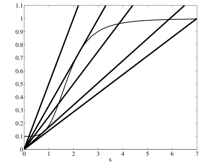
Figure 1: Schematic illustration of the possibility of one, two or three solutions of Equation 15 for varying values of $\kappa_{d}$ with inducible regulation. The monotone increasing graph is the function $f$ of Equation 10, and the straight lines correspond to $x/\kappa_{d}$ for (in a clockwise direction) $\kappa_{d}\in[0,\kappa_{d-})$, $\kappa_{d}=\kappa_{d-}$, $\kappa_{d}\in(\kappa_{d-},\kappa_{d+})$, $\kappa_{d}=\kappa_{d+}$, and $\kappa_{d+}<\kappa_{d}$. This figure was constructed with $n=4$ and $K=10$ for which $\kappa_{d-}=3.01$ and $\kappa_{d+}=5.91$ as computed from (18). See the text for further details.

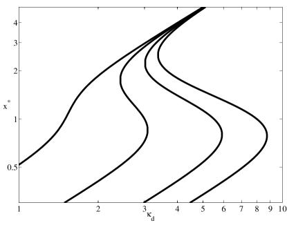
Figure 2: Full logarithmic plot of the steady state values of $x^{*}$ versus $\kappa_{d}$ for an inducible system, obtained from Equation 15, for $n=4$ and $K=2,5,10,\mbox{and}\,\,15$ (left to right) illustrating the dependence of the occurrence of bistability on $K$. See the text for details.

Analytic conditions for the existence of one or more steady states can be obtained by using Equation 15 in conjunction with the observation that the delineation points are marked by the values of $\kappa_{d}$ at which $x/\kappa_{d}$ is tangent to $f(x)$ (see Figure 1). Simple differentiation of (15) yields the second condition

$$\dfrac{1}{\kappa_{d}n(K-1)}=\dfrac{x^{n-1}}{(K+x^{n})^{2}}.$$ (16)

From equations (15) and (16) we obtain the values of $x$ at which tangency will occur:

$$x_{\pm}=\sqrt[n]{\dfrac{K-1}{2}\left\{\left[n-\dfrac{K+1}{K-1}\right]\pm\sqrt{n^{2}-2n\dfrac{K+1}{K-1}+1}\right\}}.$$ (17)

The two corresponding values of $\kappa_{d}$ at which a tangency occurs are given by

$$\kappa_{d\pm}=x_{\mp}\dfrac{K+x_{\mp}^{n}}{1+x_{\mp}^{n}}.$$ (18)

(Note the deliberate use of $x_{\mp}$ as opposed to $x_{\pm}$.)

A necessary condition for the existence of two or more steady states is obtained by requiring that the square root in (17) be non-negative, or

$$K\geq\left(\dfrac{n+1}{n-1}\right)^{2}.$$ (19)

From this a second necessary condition follows, namely

$$\kappa_{d}\geq\dfrac{n+1}{n-1}\sqrt[n]{\dfrac{n+1}{n-1}}.$$ (20)

Further, from Equations 15 and 16 we can delineate the boundaries in $(K,\kappa_{d})$ space in which there are one or three locally stable steady states as shown in Figure 3. There, we have given a parametric plot ($x$ is the parameter) of $\kappa_{d}$ versus $K$, using

$$K(x)=\dfrac{x^{n}[x^{n}+(n+1)]}{(n-1)x^{n}-1}\quad\mbox{and}\quad\kappa_{d}(x)=\dfrac{[K(x)+x^{n}]^{2}}{nx^{n-1}[K(x)-1]},$$

for $n=4$ obtained from Equations 15 and 16. As is clear from the figure, when leakage is appreciable (small $K$, e.g for $n=4$, $K<(5/3)^{2}$) then the possibility of bistable behaviour is lost.

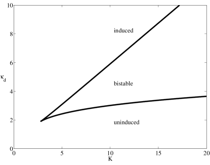
Figure 3: In this figure we present a parametric plot (for $n=4$) of the bifurcation diagram in $(K,\kappa_{d})$ parameter space delineating one from three steady states in a deterministic inducible operon as obtained from Equations 15 and 16. The upper (lower) branch corresponds to $\kappa_{d-}$ ($\kappa_{d+}$), and for all values of $(K,\kappa_{d})$ in the interior of the cone there are two locally stable steady states $X_{1}^{*},X_{3}^{*}$, while outside there is only one. The tip of the cone occurs at $(K,\kappa_{d})=((5/3)^{2},(5/3)\sqrt[4]{5/3})$ as given by Equations 19 and 20. For $K\in[0,(5/3)^{2})$ there is but a single steady state.

Remark 1.

Some general observations on the influence of $n$, $K$, and $\kappa_{d}$ on the appearance of bistability in the deterministic case are in order.

1. The degree of cooperativity $(n)$ in the binding of effector to the repressor plays a significant role. Indeed, $n>1$ is a necessary condition for bistability.

2. If $n>1$ then a second necessary condition for bistability is that $K$ satisfies Equation 19 so the fractional leakage $(K^{-1})$ is sufficiently small.

3. Furthermore, $\kappa_{d}$ must satisfy Equation 20 which is quite instructive. Namely for $n\to\infty$ the limiting lower limit is $\kappa_{d}>1$ while for $n\to 1$ the minimal value of $\kappa_{d}$ becomes quite large. This simply tells us that the ratio of the product of the production rates to the product of the degradation rates must always be greater than 1 for bistability to occur, and the lower the degree of cooperativity $(n)$ the larger the ratio must be.

4. If $n$, $K$ and $\kappa_{d}$ satisfy these necessary conditions then bistability is only possible if $\kappa_{d}\in[\kappa_{d-},\kappa_{d+}]$ (c.f. Figure 3).

5. The locations of the minimal $(x_{-})$ and maximal $(x_{+})$ values of $x$ bounding the bistable region are independent of $\kappa_{d}$.

6. Finally

   1. $(x_{+}-x_{-})$ is a decreasing function of increasing $n$ for constant $\kappa_{d},K$

   2. $(x_{+}-x_{-})$ is an increasing function of increasing $K$ for constant $n,\kappa_{d}$.

Local and global stability. The local stability of a steady state $x^{*}$ is determined by the solutions of the eigenvalue equation (Yildirim et al., 2004)

$$(\lambda+\gamma_{1})(\lambda+\gamma_{2})(\lambda+\gamma_{3})-\gamma_{1}\gamma_{2}\gamma_{3}\kappa_{d}f^{\prime}_{*}=0,\quad f^{\prime}_{*}=f^{\prime}(x^{*}).$$ (21)

Set

$$a_{1}=\sum_{i=1}^{3}\gamma_{i},\quad a_{2}=\sum_{i\neq j=1}^{3}\gamma_{i}\gamma_{j},\quad a_{3}=(1-\kappa_{d}f^{\prime}_{*})\prod_{i=1}^{3}\gamma_{i},$$

so (21) can be written as

$$\lambda^{3}+a_{1}\lambda^{2}+a_{2}\lambda+a_{3}=0.$$ (22)

By Descartes’s rule of signs, (22) will have either no positive roots for $f^{\prime}_{*}\in[0,\kappa_{d}^{-1})$ or one positive root otherwise. With this information and using the notation SN to denote a locally stable node, HS a half or neutrally stable steady state, and US an unstable steady state (saddle point), then there will be:

• A single steady state $X_{1}^{*}$ (SN), for $\kappa_{d}\in[0,\kappa_{d-})$

• Two coexisting steady states $X_{1}^{*}$ (SN) and $X_{2}^{*}=X_{3}^{*}$ (HS, born through a saddle node bifurcation) for $\kappa_{d}=\kappa_{d-}$

• Three coexisting steady states $X_{1}^{*}(SN),X_{2}^{*}(US),X_{3}^{*}$ (SN) for $\kappa_{d}\in(\kappa_{d-},\kappa_{d+})$

• Two coexisting steady states $X_{1}^{*}=X_{2}^{*}$ (HS at a saddle node bifurcation), and $X_{3}^{*}$ (SN) for $\kappa_{d}=\kappa_{d+}$

• One steady state $X_{3}^{*}$ (SN) for $\kappa_{d+}<\kappa_{d}$.

For the inducible operon, other work extends these local stability considerations and we have the following result characterizing the global behaviour:

Theorem 1.

(Othmer, 1976; Smith, 1995, Proposition 2.1, Chapter 4) For an inducible operon with $\varphi$ given by Equation 3, define $I_{I}=[1/K,1]$. There is an attracting box $B_{I}\subset\mathbb{R}_{3}^{+}$ defined by

$$B_{I}=\{(x_{1},x_{2},x_{3}):x_{i}\in I_{I},\,\,i=1,2,3\}$$

such that the flow $S_{t}$ is directed inward everywhere on the surface of $B_{I}$. Furthermore, all $X^{*}\in B_{I}$ and

1. If there is a single steady state, i.e. $X_{1}^{*}$ for $\kappa_{d}\in[0,\kappa_{d-})$, or $X_{3}^{*}$ for $\kappa_{d+}<\kappa_{d}$, then it is globally stable.

2. If there are two locally stable nodes, i.e. $X_{1}^{*}$ and $X_{3}^{*}$ for $\kappa_{d}\in(\kappa_{d-},\kappa_{d+})$, then all flows $S(X^{0})$ are attracted to one of them. (See Selgrade (1979) for a delineation of the basin of attraction of $X_{1}^{*}$ and $X_{3}^{*}$.)

2.3.3 Repressible regulation

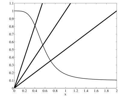
Figure 4: Schematic illustration that there is only a single solution of Equation 15 for all values of $\kappa_{d}$ with repressible regulation. The monotone decreasing graph is $f$ for a repressible operon, while the straight lines are $x/\kappa_{d}$. This figure was constructed with $n=4$ and $\Delta=10$. See the text for further details.

As illustrated in Figure 4, the repressible operon has a single steady state corresponding to the unique solution $x^{*}$ of Equation 15. To determine its local stability we apply the Routh-Hurwitz criterion to the eigenvalue equation (22). The steady state corresponding to $x^{*}$ will be locally stable (i.e. have eigenvalues with negative real parts) if and only if $a_{1}>0$ (always the case) and

$$a_{1}a_{2}-a_{3}>0.$$ (23)

The well known relation between the arithmetic and geometric means

$$\dfrac{1}{n}\sum_{i=1}^{n}\gamma_{i}\geq\left(\prod_{i=1}^{n}\gamma i\right)^{1/n},$$

when applied to both $a_{1}$ and $a_{2}$ gives, in conjunction with Equation 23,

$$a_{1}a_{2}-a_{3}\geq(8+\kappa_{d}f^{\prime}_{*})\prod_{i=1}^{3}\gamma_{i}>0.$$

Thus as long as $f^{\prime}_{*}>-8/\kappa_{d}$, the steady state corresponding to $x^{*}$ will be locally stable. Once condition (23) is violated, stability of $x^{*}$ is lost via a supercritical Hopf bifurcation and a limit cycle is born. One may even compute the Hopf period of this limit cycle by assuming that $\lambda=j\omega_{H}$ ($j=\sqrt{-1}$) in Equation 22 where $\omega_{H}$ is the Hopf angular frequency. Equating real and imaginary parts of the resultant yields $\omega_{H}=\sqrt{a_{3}/a_{1}}$ or

$$T_{H}=\dfrac{2\pi}{\omega_{H}}={2\pi}\times\sqrt{\dfrac{\sum_{i=1}^{3}\gamma_{i}}{(1-\kappa_{d}f^{\prime}_{*})\prod_{i=1}^{3}\gamma_{i}}}.$$

These local stability results tell us nothing about the global behaviour when stability is lost, but it is possible to characterize the global behaviour of a repressible operon with the following

Theorem 2.

(Smith, 1995, Theorem 4.1 & Theorem 4.2, Chapter 3) For a repressible operon with $\varphi$ given by Equation 4, define $I_{R}=[K_{1}/K,1]$. There is a globally attracting box $B_{R}\subset\mathbb{R}_{3}^{+}$ defined by

$$B_{R}=\{(x_{1},x_{2},x_{3}):x_{i}\in I_{R},\,\,i=1,2,3\}$$

such that the flow $S$ is directed inward everywhere on the surface of $B_{R}$. Furthermore there is a single steady state $X^{*}\in B_{R}$. If $X^{*}$ is locally stable it is globally stable, but if $X^{*}$ is unstable then a generalization of the Poincare-Bendixson theorem (Smith, 1995, Chapter 3) implies the existence of a globally stable limit cycle in $B_{R}$.

Remark 2.

There is no necessary connection between the Hopf period computed from the local stability analysis and the period of the globally stable limit cycle.

3 Fast and slow variables

In dynamical systems, considerable simplification and insight into the behaviour can be obtained by identifying fast and slow variables. This technique is especially useful when one is initially interested in the approach to a steady state. In this context a fast variable is one that relaxes much more rapidly to an equilibrium than a slow variable (Haken, 1983). In many systems, including chemical and biochemical ones, this is often a consequence of differences in degradation rates, with the fastest variable the one that has the largest degradation rate. We employ the same strategy here to obtain approximations to the population level dynamics that will be used in the next section.

It is often the case that the degradation rate of mRNA is much greater than the corresponding degradation rates for both the intermediate protein and the effector $(\gamma_{1}\gg\gamma_{2},\gamma_{3})$ so in this case the mRNA dynamics are fast and we have the approximate relationship

$$x_{1}\simeq\kappa_{d}f(x_{3}).$$

Consequently the three variable system describing the generic operon reduces to a two variable one involving the slower intermediate and effector:

$$\dfrac{dx_{2}}{dt} =\gamma_{2}[\kappa_{d}f(x_{3})-x_{2}],$$ (24)

$$\dfrac{dx_{3}}{dt} =\gamma_{3}(x_{2}-x_{3}).$$ (25)

In our considerations of specific single operon dynamics below we will also have occasion to examine two further subcases, namely

Case 1. Intermediate (protein) dominated dynamics. If it should happen that $\gamma_{1}\gg\gamma_{3}\gg\gamma_{2}$ (as for the lac operon, then the effector also qualifies as a fast variable so

$$x_{3}\simeq x_{2}$$

and thus from (24)-(25) we recover the one dimensional equation for the slowest variable, the intermediate:

$$\dfrac{dx_{2}}{dt}=\gamma_{2}[\kappa_{d}f(x_{2})-x_{2}].$$ (26)

Case 2. Effector (enzyme) dominated dynamics. Alternately, if $\gamma_{1}\gg\gamma_{2}\gg\gamma_{3}$ then the intermediate is a fast variable relative to the effector and we have

$$x_{2}\simeq x_{3}$$

so our two variable system ( 24)-(25) reduces to a one dimensional system

$$\dfrac{dx_{3}}{dt}=\gamma_{3}[\kappa_{d}f(x_{3})-x_{3}]$$ (27)

for the relatively slow effector dynamics.

Both Equations 26 and 27 are of the form

$$\dfrac{dx}{dt}=\gamma[\kappa_{d}f(x)-x]$$ (28)

where $\gamma$ is either $\gamma_{2}$ for protein ($x_{2}$) dominated dynamics or $\gamma_{3}$ for effector ($x_{3}$) dominated dynamics.

4 Distributions with intrinsic bursting

4.1 Generalities

It is well documented experimentally (Cai et al., 2006; Chubb et al., 2006; Golding et al., 2005; Raj et al., 2006; Sigal et al., 2006; Yu et al., 2006) that in some organisms the amplitude of protein production through bursting translation of mRNA is exponentially distributed at the single cell level with density

$$h(y)=\dfrac{1}{\bar{b}}e^{-y/{\bar{b}}},$$ (29)

where $\bar{b}$ is the average burst size, and that the frequency of bursting $\varphi$ is dependent on the level of the effector. Writing Equation 29 in terms of our dimensionless variables we have

$$h(x)=\dfrac{1}{b}e^{-x/{b}}.$$ (30)

Remark 3.

The technique of eliminating fast variables described in Section 2.3 above (also known as the adiabatic elimination technique (Haken, 1983)) has been extended to stochastically perturbed systems when the perturbation is a Gaussian distributed white noise, c.f. Stratonovich (1963, Chapter 4, Section 11.1), Wilemski (1976), Titular (1978), and Gardiner (1983, Section 6.4). However, to the best of our knowledge, this type of approximation has never been extended to the situation dealt with here in which the perturbation is a jump Markov process.

The single cell analog of the population level intermediate protein dominated Case 1 above (when $\gamma_{1}\gg\gamma_{3}\gg\gamma_{2}$) is

$$\dfrac{dx_{2}}{dt}=-\gamma_{2}x_{2}+\Xi(h,\varphi(x_{2})),\quad\mbox{with}\quad\varphi(x_{2})=\gamma_{2}\varphi_{m}f(x_{2}),$$ (31)

where $\Xi(h,\varphi)$ denotes a jump Markov process, occurring at a rate $\varphi$, whose amplitude is distributed with density $h$ as given in (30). Analogously, in the Case 2 effector dominated situation the single cell equation becomes

$$\dfrac{dx_{3}}{dt}=-\gamma_{3}x_{3}+\Xi(h,\varphi(x_{3})),\quad\mbox{with}\quad\varphi(x_{3})=\gamma_{3}\varphi_{m}f(x_{3}).$$ (32)

Equations 31 and 32 can both be written as

$$\dfrac{dx}{dt}=-\gamma x+\Xi(h,\varphi(x)),\quad\mbox{with}\quad\varphi(x)=\gamma\kappa_{b}f(x),\,\,\kappa_{b}\equiv\varphi_{m}.$$

Remark 4.

In the case of bursting we will always take $\kappa_{b}\equiv\varphi_{m}$ in contrast to the deterministic case where $\kappa_{d}=b_{d}\varphi_{m}$.

From Mackey and Tyran-Kamińska (2008) the corresponding operator equation for the evolution of the density $u(t,x)$ when there is a single dominant slow variable is given by

$$\begin{split}\dfrac{\partial u(t,x)}{\partial t}-\gamma\dfrac{\partial(xu(t,x))}{\partial x}&=-\gamma\kappa_{b}f(x)u(t,x)\\ &\quad+\gamma\kappa_{b}\int_{0}^{x}f(y)u(t,y)h(x-y)dy.\end{split}$$ (33)

Remark 5.

This is a straightforward generalization of what Gardiner (1983, Section 3.4) refers to as the differential Chapman-Kolmogorov equation.

Stationary solutions $u_{*}(x)$ of (33) are solutions of

$$-\dfrac{d(xu_{*}(x))}{dx}=-\kappa_{b}f(x)u_{*}(x)+\kappa_{b}\int_{0}^{x}f(y)u_{*}(y)h(x-y)dy.$$ (34)

If there is a unique stationary density, then the solution $u(t,x)$ of Equation 33 is said to be asymptotically stable (Lasota and Mackey, 1994) in the sense that

$$\lim_{t\to\infty}\int_{0}^{\infty}|u(t,x)-u_{*}(x)|dx=0$$

for all initial densities $u(0,x)$.

Theorem 3.

(Mackey and Tyran-Kamińska, 2008, Theorem 7). The unique stationary density of Equation 34, with $f$ given by Equation 9 and $h$ given by (29), is

$$u_{*}(x)=\dfrac{\mathcal{C}}{x}e^{-x/b}\exp\left[\kappa_{b}\int^{x}\frac{f(y)}{y}dy\right],$$ (35)

where $\mathcal{C}$ is a normalizing constant such that $\int_{0}^{\infty}u_{*}(x)dx=1$. Further, $u(t,x)$ is asymptotically stable.

Remark 6.

The stationary density (35) is found by rewriting Equation 34 in the form

$$\dfrac{dy(x)}{dx}+\dfrac{y(x)}{b}-\kappa_{b}\dfrac{f(x)}{x}y(x)=0,\quad y(x)\equiv xu_{*}(x)$$

using Laplace transforms and solving by quadratures. Note also that we can represent $u_{*}$ as

$$u_{*}(x)=\mathcal{C}\exp\int^{x}\left(\frac{\kappa_{b}f(y)}{y}-\frac{1}{b}-\frac{1}{y}\right)dy,$$

where $\mathcal{C}$ is a normalizing constant.

4.2 Distributions in the presence of bursting

4.2.1 Protein distribution in the absence of control

If the burst frequency $\varphi=\gamma\kappa_{b}f$ is independent of the level of all of the participating molecular species, then the solution given in Equation 35 is the density of the gamma distribution:

$$u_{*}(x)=\dfrac{1}{b^{\kappa_{b}}\Gamma(\kappa_{b})}x^{\kappa_{b}-1}e^{-x/b},$$

where $\Gamma(\cdot)$ denotes the gamma function. For $\kappa_{b}\in(0,1)$, $u_{*}(0)=\infty$ and $u_{*}$ is decreasing while for $\kappa_{b}>1$, $u_{*}(0)=0$ and there is a maximum at $x=b(\kappa_{b}-1)$.

4.2.2 Controlled bursting

We next consider the situation in which the burst frequency $\varphi$ is dependent on the level of $x$, c.f. Equation 5. This requires that we evaluate

$$\begin{split}\kappa_{b}\int^{x}\dfrac{f(y)}{y}dy=\int^{x}\dfrac{\kappa_{b}}{y}\left[\dfrac{1+y^{n}}{\Lambda+\Delta y^{n}}\right]dy=\ln\left\{x^{\kappa_{b}\Lambda^{-1}}(\Lambda+\Delta x^{n})^{\theta}\right\},\end{split}$$

where $\Lambda,\Delta$ are enumerated in Table 1 for both the inducible and repressible operons treated in Section 2.2 and

$$\theta=\frac{\kappa_{b}}{n\Delta}\left(1-\frac{\Delta}{\Lambda}\right).$$

Consequently, the steady state density (35) explicitly becomes

$$u_{*}(x)={\mathcal{C}}e^{-x/b}x^{\kappa_{b}\Lambda^{-1}-1}(\Lambda+\Delta x^{n})^{\theta}.$$ (36)

The first two terms of Equation 36 are simply proportional to the density of the gamma distribution. For $0<\kappa_{b}\Lambda^{-1}<1$ we have $u_{*}(0)=\infty$ while for $\kappa_{b}\Lambda^{-1}>1$, $u_{*}(0)=0$ and there is at least one maximum at a value of $x>0$. We have $u_{*}(x)>0$ for all $x>0$ and from Remark 6 it follows that

$$u_{*}^{\prime}(x)=u_{*}(x)\left(\frac{\kappa_{b}f(x)}{x}-\frac{1}{b}-\frac{1}{x}\right),\quad x>0.$$ (37)

Observe that if $\kappa_{b}\leq 1$ then $u_{*}$ is a monotone decreasing function of $x$, since $\kappa_{b}f(x)\leq 1$ for all $x>0$. Thus we assume in what follows that $\kappa_{b}>1$.

Since the analysis of the qualitative nature of the stationary density leads to different conclusions for the inducible and repressible operon cases, we consider each in turn.

4.2.3 Bursting in the inducible operon

For $\theta>0$, as in the case of an inducible operon, the third term of Equation 36 is a monotone increasing function of $x$ and, consequently, there is the possibility that $u_{*}$ may have more than one maximum, indicative of the existence of bistable behaviour. In this case, the stationary density becomes

$$u_{*}(x)={\mathcal{C}}e^{-x/b}x^{\kappa_{b}K^{-1}-1}(K+x^{n})^{\theta},\quad\theta=\dfrac{\kappa_{b}}{n}(1-K^{-1}).$$

From (37) it follows that we have $u_{*}^{\prime}(x)=0$ for $x>0$ if and only if

$$\dfrac{1}{\kappa_{b}}\left(\dfrac{x}{b}+1\right)=\dfrac{1+x^{n}}{K+x^{n}}.$$ (38)

Again, graphical arguments (see Figure 5) show that there may be up to three roots of (38).

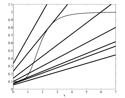
Figure 5: Schematic illustration of the possibility of one, two or three solutions of Equation 38 for varying values of $\kappa_{b}$ with bursting inducible regulation. The straight lines correspond (in a clockwise direction) to $\kappa_{b}\in(0,\kappa_{b-})$, $\kappa_{b}=\kappa_{b-}$, $\kappa_{b}\in(\kappa_{b-},\kappa_{b+})$ (and respectively $\kappa_{b}<K$, $\kappa_{b}=K$, $K<\kappa_{b}$), $\kappa_{b}=\kappa_{b+}$, and $\kappa_{b+}<\kappa_{b}$. This figure was constructed with $n=4$, $K=10$ and $b=1$ for which $\kappa_{b-}=4.29$ and $\kappa_{b+}=14.35$ as computed from (42). See the text for further details.

For illustrative values of $n$, $K$, and $b$, Figure 6 shows the graph of the values of $x$ at which $u_{*}^{\prime}(x)=0$ as a function of $\kappa_{b}$. When there are three roots of (38), we label them as $\tilde{x}_{1}<\tilde{x}_{2}<\tilde{x}_{3}$.

Generally we cannot determine when there are three roots. However, we can determine when there are only two roots $\tilde{x}_{1}<\tilde{x}_{3}$ from the argument of Section 2.3.2. At $\tilde{x}_{1}$ and $\tilde{x}_{3}$ we will not only have Equation 38 satisfied but the graph of the right hand side of (38) will be tangent to the graph of the left hand side at one of them so the slopes will be equal. Differentiation of (38) yields the second condition

$$n\dfrac{x^{n-1}}{(K+x^{n})^{2}}=\dfrac{1}{\kappa_{b}b(K-1)}$$ (39)

We first show that there is an open set of parameters $(b,K,\kappa_{b})$ for which the stationary density $u_{*}$ is bimodal. From Equations 38 and 39 it follows that the value of $x_{\pm}$ at which tangency will occur is given by

$$x_{\pm}=b(\kappa_{b}-1)z_{\pm}$$

and $z_{\pm}$ are positive solutions of equation

$$\frac{z}{n}=1-z-\beta(1-z)^{2},\quad\text{where}\quad\beta=\frac{K(\kappa_{b}-1)}{(K-1)\kappa_{b}}.$$

We explicitly have

$$z_{\pm}=\frac{1}{2\beta n}\left(2\beta n-\left(n+1\right)\pm\sqrt{\left(n+1\right)^{2}-4\beta n}\right)$$

provided that

$$\frac{(n+1)^{2}}{4n}\geq\beta=\frac{K(\kappa_{b}-1)}{(K-1)\kappa_{b}}.$$ (40)

Equation 40 is always satisfied when $\kappa_{b}<K$ or when $\kappa_{b}>K$ and $K$ is as in the deterministic case (19). Observe also that we have $z_{+}>0>z_{-}$ for $\kappa_{b}<K$ and $z_{+}>z_{-}>0$ for $\kappa_{b}>K$. The two corresponding values of $b$ at which a tangency occurs are given by

$$b_{\pm}=\frac{1}{(\kappa_{b}-1)z_{\pm}}\sqrt[n]{\frac{K}{\beta(1-z_{\pm})}-K}\quad\text{and}\quad z_{\pm}>0.$$

If $\kappa_{b}<K$ then $u_{*}(0)=\infty$ and $u_{*}$ is decreasing for $b\leq b_{+}$, while for $b>b_{+}$ there is a local maximum at $x>0$. If $\kappa_{b}>K$ then $u_{*}(0)=0$ and $u_{*}$ has one or two local maximum. As a consequence, for $n>1$ we have a bimodal steady state density $u_{*}$ if and only if the parameters $\kappa_{b}$ and $K$ satisfy (40), $\kappa_{b}>K$, and $b\in(b_{+},b_{-})$.

We now want to find the analogy between the bistable behavior in the deterministic system and the existence of bimodal stationary density $u_{*}$. To this end we fix the parameters $b>0$ and $K>1$ and vary $\kappa_{b}$ as in Figure 5. Equations 38 and 39 can also be combined to give an implicit equation for the value of $x_{\pm}$ at which tangency will occur

$$x^{2n}-(K-1)\left[n-\dfrac{K+1}{K-1}\right]x^{n}-nb(K-1)x^{n-1}+K=0$$ (41)

and the corresponding values of $\kappa_{b\pm}$ are given by

$$\kappa_{b\pm}=\left(\dfrac{x_{\mp}+b}{b}\right)\left(\dfrac{K+x_{\mp}^{n}}{1+x_{\mp}^{n}}\right).$$ (42)

There are two cases to distinguish.

Case 1. $0<\kappa_{b}<K$. In this case, $u_{*}(0)=\infty$. Further, the same graphical considerations as in the deterministic case show that there can be none, one, or two positive solutions to Equation 38. If $\kappa_{b}<\kappa_{b-}$, there are no positive solutions, $u_{*}$ is a monotone decreasing function of $x$. If $\kappa_{b}>\kappa_{b-}$, there are two positive solutions ($\tilde{x}_{2}$ and $\tilde{x}_{3}$ in our previous notation, $\tilde{x}_{1}$ has become negative and not of importance) and there will be a maximum in $u_{*}$ at $\tilde{x}_{3}$ with a minimum in $u_{*}$ at $\tilde{x}_{2}$.

Case 2. $0<K<\kappa_{b}$. Now, $u_{*}(0)=0$ and there may be one, two, or three positive roots of Equation 38. We are interested in knowing when there are three which we label as $\tilde{x}_{1}<\tilde{x}_{2}<\tilde{x}_{3}$ as $\tilde{x}_{1},\tilde{x}_{3}$ will correspond to the location of maxima in $u_{*}$ while $\tilde{x}_{2}$ will be the location of the minimum between them and the condition for the existence of three roots is $\kappa_{b-}<\kappa_{b}<\kappa_{b+}$.

We see then that the different possibilities depend on the respective values of $K$, $\kappa_{b-}$, $\kappa_{b+}$, and $\kappa_{b}$. To summarize, we may characterize the stationary density $u_{*}$ for an inducible operon in the following way:

1. Unimodal type 1: $u_{*}(0)=\infty$ and $u_{*}$ is decreasing for $0<\kappa_{b}<\kappa_{b-}$ and $0<\kappa_{b}<K$

2. Unimodal type 2: $u_{*}(0)=0$ and $u_{*}$ has a single maximum at

   1. $\tilde{x}_{1}>0$ for $K<\kappa_{b}<\kappa_{b-}$ or

   2. at $\tilde{x}_{3}>0$ for $\kappa_{b+}<\kappa_{b}$ and $K<\kappa_{b}$

3. Bimodal type 1: $u_{*}(0)=\infty$ and $u_{*}$ has a single maximum at $\tilde{x}_{3}>0$ for $\kappa_{b-}<\kappa_{b}<K$

4. Bimodal type 2: $u_{*}(0)=0$ and $u_{*}$ has two maxima at $\tilde{x}_{1},\tilde{x}_{3}$, $0<\tilde{x}_{1}<\tilde{x}_{3}$ for $\kappa_{b-}<\kappa_{b}<\kappa_{b+}$ and $K<\kappa_{b}$

Remark 7.

Remember that the case $n=1$ cannot display bistability in the deterministic case. However, in the case of bursting in the inducible system when $n=1$, if $\frac{K}{b}+1<\kappa_{b}<K$ and $b>\frac{K}{K-1}$, then $u_{*}(0)=\infty$ and $u_{*}$ also has a maximum at $\tilde{x}_{3}>0$. Thus in this case one can have a Bimodal type 1 stationary density.

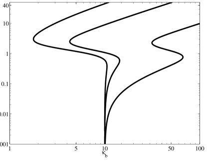
Figure 6: Full logarithmic plot of the values of $x$ at which $u_{*}^{\prime}(x)=0$ versus the parameter $\kappa_{b}$, obtained from Equation 38, for $n=4$, $K=10$, and (left to right) $b=5,1$ and $b=\frac{1}{10}$. Though somewhat obscured by the logarithmic scale for $x$, the graphs always intersect the $\kappa_{b}$ axis at $\kappa_{b}=K$. Additionally, it is important to note that $u^{\prime}_{*}(0)=0$ for $K<\kappa_{b}$, and that there is always a maximum at $0$ for $0<\kappa_{b}<K$. See the text for further details.

We now choose to see how the average burst size $b$ affects bistability in the density $u_{*}$ by looking at the parametric plot of $\kappa_{b}(x)$ versus $K(x)$. Define

$$F(x,b)=\dfrac{x^{n}+1}{nx^{n-1}(x+b)}.$$ (43)

Then

$$K(x,b)=\dfrac{1+x^{n}F(x,b)}{1-F(x,b)}\quad\mbox{and}\quad\kappa_{b}(x,b)=[K(x,b)+x^{n}]\dfrac{x+b}{b(x^{n}+1)}.$$ (44)

The bifurcation diagram obtained from a parametric plot of $K$ versus $\kappa_{b}$ (with $x$ as the parameter) is illustrated in Figure 7 for $n=4$ and two values of $b$. Note that it is necessary for $0<K<\kappa_{b}$ in order to obtain Bimodal type 2 behaviour.

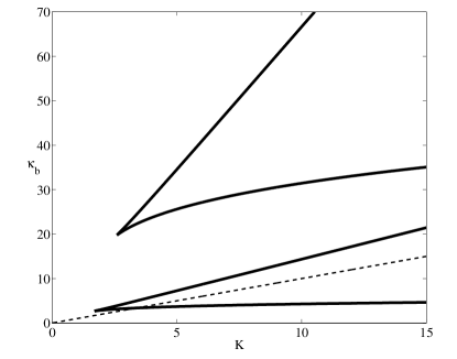
Figure 7: In this figure we present two bifurcation diagrams (for $n=4$) in $(K,\kappa_{b})$ parameter space delineating unimodal from bimodal stationary densities $u_{*}$ in an inducible operon with bursting as obtained from Equations 44 with 43. The upper cone-shaped plot is for $b=\frac{1}{10}$ while the bottom one is for $b=1$. In both cone shaped regions, for any situation in which the lower branch is above the line $\kappa_{b}=K$ (lower straight line) then bimodal behaviour in the stationary solution $u_{*}(x)$ will be observed with maxima in $u_{*}$ at positive values of $x$, $\tilde{x}_{1}$ and $\tilde{x}_{3}$.

For bursting behaviour in an inducible situation, there are two different bifurcation patterns that are possible. The two different cases are delineated by the respective values of $K$ and $\kappa_{b}$, as shown in Figure 6 and Figure 7. Both bifurcation scenarios share the property that while increasing the bifurcation parameter $\kappa_{b}$ from $0$ to $\infty$, the stationary density $u_{*}$ passes from a unimodal density with a peak at a low value (either $0$ or $\tilde{x}_{1}$) to a bimodal density and then back to a unimodal density with a peak at a high value ($\tilde{x}_{3}$).

In what will be referred as Bifurcation type 1, the maximum at $x=0$ disappears when there is a second peak at $x=\tilde{x}_{3}$. The sequence of densities encountered for increasing values of $\kappa_{b}$ is then: Unimodal type 1 to a Bimodal type 1 to a Bimodal type 2 and finally to a Unimodal type 2 density.

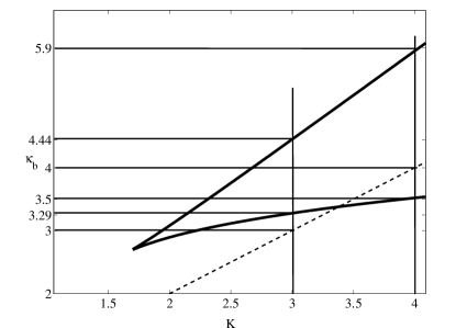
Figure 8: This figure presents an enlarged portion of Figure 7 for $b=1$. The various horizontal lines mark specific values of $\kappa_{b}$ referred to in Figures 9 and 10.

In the Bifurcation type 2 situation, the sequence of density types for increasing values of $\kappa_{b}$ is: Unimodal type 1 to a Unimodal type 2 and then a Bimodal type 2 ending in a Unimodal type 2 density.

The two different kinds of bifurcation that can occur are easily illustrated for $b=1$ as the parameter $\kappa_{b}$ is increased. (An enlarged diagram in the region of interest is shown in Figure 8.) Figure 9 illustrates Bifurcation type 1, when $K=4$, and $\kappa_{b}$ increases from low to high values. As $\kappa_{b}$ increases, we pass from a Unimodal type 1 density, to a Bimodal type 1 density. Further increases in $\kappa_{b}$ lead to a Bimodal type 2 density and finally to a Unimodal type 2 density. This bifurcation cannot occur, for example, when $b=\frac{1}{10}$ and $K\leq 15$ (see Figure 7).

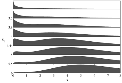
Figure 9: In this figure we illustrate Bifurcation type 1 when intrinsic bursting is present. For a variety of values of the bifurcation parameter $\kappa_{b}$ (between $3$ and $6$ from top to down), the stationary density $u_{*}$ is plotted versus $x$ between $0$ and $8$. The values of the parameters used in this figure are $b=1$, $K=4$, and $n=4$. For $\kappa_{b}\lesssim 3.5$, $u_{*}$ has a single maximum at $x=0$. For $3.5\lesssim\kappa_{b}<4$, $u_{*}$ has two local maxima at $x=0$ and $\tilde{x}_{3}>1$. For $4<\kappa_{b}\lesssim 5.9$, $u_{*}$ has two local maxima at $0<\tilde{x}_{1}<\tilde{x}_{3}$. Finally, for $\kappa_{b}\gtrsim 5.9$, $u_{*}$ has a single maximum at $\tilde{x}_{3}>1$. Note that for each plot of the density, the scale of the ordinate is arbitrary to improve the visualization.

Figure 10 shows Bifurcation type 2, when $K=3$. As $\kappa_{b}$ increases, we pass from a Unimodal type 1 density, to a Unimodal type 2 density. Then with further increases in $\kappa_{b}$, we pass to a Bimodal type 2 density and finally back to a Unimodal type 2 density.

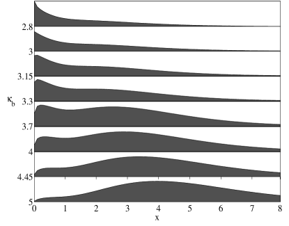
Figure 10: An illustration of Bifurcation type 2 for intrinsic bursting. For several values of the bifurcation parameter $\kappa_{b}$ (between $2.8$ and $5$ from top to down), the stationary density $u_{*}$ is plotted versus $x$ between $0$ and $8$. The parameters used are $b=1$, $K=3$, and $n=4$. For $\kappa_{b}<3$, $u_{*}$ has a single maximum at $x=0$, and for $3<\kappa_{b}\lesssim 3.3$, $u_{*}$ has a single maximum at $\tilde{x}_{1}>0$. For $3.3\lesssim\kappa_{b}\lesssim 4.45$, $u_{*}$ has two local maxima at $0<\tilde{x}_{1}<\tilde{x}_{3}$, and finally for $\kappa_{b}\gtrsim 4.45$ $u_{*}$ has a single maximum at $\tilde{x}_{3}>0$. Note that for each plot of the density, the scale of the ordinate is abritrary to improve the visualization.

Remark 8.

There are several qualitative conclusions to be drawn from the analysis of this section.

1. The presence of bursting can drastically alter the regions of parameter space in which bistability can occur relative to the deterministic case. Figure 11 presents the regions of bistability in the presence of bursting in the $(K,b\cdot\kappa_{b})$ parameter space, which should be compared to the region of bistability in the deterministic case in the $(K,\kappa_{d})$ parameter space ($b\kappa_{b}$ is the mean number of proteins produced per unit of time, as is $\kappa_{d}$)

2. When $0<\kappa_{b}<K$, at a fixed value of $\kappa_{b}$, increasing the average burst size $b$ can lead to a bifurcation from Unimodal type 1 to Bimodal type 1.

3. When $0<K<\kappa_{b}$, at a fixed value of $\kappa_{b}$, increasing $b$ can lead to a bifurcation from Unimodal type 2 to Bimodal type 2 and then back to Unimodal type 2.

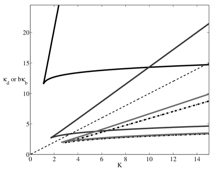
Figure 11: The presence of bursting can drastically alter regions of bimodal behaviour as shown in this parametric plot (for $n=4$) of the boundary in $(K,b\cdot\kappa_{b})$ parameter space delineating unimodal from bimodal stationary densities $u_{*}$ in an inducible operon with bursting and in $(K,\kappa_{d})$ parameter space delineating one from three steady states in the deterministic inducible operon. From top to bottom, the regions are for $b=10$, $b=1$, $b=0.1$ and $b=0.01$. The lowest (heavy dashed line) is for the deterministic case. Note that for $b=0.1$, the two regions of bistability and bimodality coincide and are indistinguishable from one another.

4.2.4 Bursting in the repressible operon

The possible behaviours in the stationary density $u_{*}$ for the repressible operon are easy to delineate based on the analysis of the previous section, with Equation 38 replaced by

$$\dfrac{1}{\kappa_{b}}\left(\dfrac{x}{b}+1\right)=\dfrac{1+x^{n}}{1+\Delta x^{n}}.$$ (45)

Again graphical arguments (see Figure 12) show that Equation 45 may have either none or one solution. Namely,

1. For $0<\kappa_{b}<1$, $u_{*}(0)=\infty$ and $u_{*}$ is decreasing. Equation 45 does not have any solution (Unimodal type 1).

2. For $1<\kappa_{b}$, $u_{*}(0)=0$ and $u_{*}$ has a single maximum at a value of $x>0$ determined by the single positive solution of Equation 45 (Unimodal type 2).

4.3 Recovering the deterministic case

We can recover the deterministic behaviour from the bursting dynamics with a suitable scaling of the parameters and limiting procedure. With bursting production there are two important parameters (the frequency $\kappa_{b}$ and the amplitude $b$), while with deterministic production there is only $\kappa_{d}$. The natural limit to consider is when

$$b\to 0,\quad\kappa_{b}\to\infty\quad\mbox{with}\quad b\kappa_{b}\equiv\kappa_{d}.$$

In this limit, the implicit equations which define the maximum points of the steady state density, become the implicit equations (15) and (16) which define the stable steady states in the deterministic case.

The bifurcations will also take place at the same points, because we recover Equation 18 in the limit. However, Bimodality type 1 as well as the Unimodal type 1 behaviours will no longer be present, as in the deterministic case, because for $\kappa_{b}\to\infty$ we have $\kappa_{b}>K$. Finally, from the analytical expression for the steady-state density (36) $u_{*}$ will became more sharply peaked as $b\to 0$. Due to the normalization constant (which depends on $b$ and $\kappa_{b}$), the mass will be more concentrated around the larger maximum of $u_{*}$.

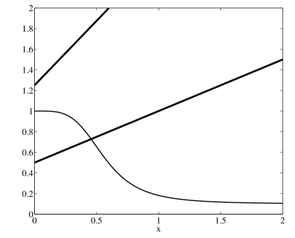
Figure 12: Schematic illustration that there can be one or no solution of Equation 45, depending on the value of $\kappa_{b}$, with repressible regulation. The straight lines correspond (in a clockwise direction) to $\kappa_{b}=2$ and $\kappa_{b}=0.8$. This figure was constructed with $n=4$, $\Delta=10$ and $b=1$. See the text for further details.

5 Distributions with fluctuations in the degradation rate

5.1 Generalities

For a generic one dimensional stochastic differential equation of the form

$$dx(t)=\alpha(x)dt+\sigma(x)dw(t)$$

the corresponding Fokker Planck equation

$$\dfrac{\partial u}{\partial t}=-\dfrac{\partial(\alpha u)}{\partial x}+\dfrac{1}{2}\dfrac{\partial^{2}(\sigma^{2}u)}{\partial x^{2}}$$ (46)

can be written in the form of a conservation equation

$$\dfrac{\partial u}{\partial t}+\dfrac{\partial J}{\partial x}=0,$$

where

$$J=\alpha u-\frac{1}{2}\dfrac{\partial(\sigma^{2}u)}{\partial x}$$

is the probability current. In a steady state when $\partial_{t}u\equiv 0$, the current must satisfy $J=\mbox{constant}$ throughout the domain of the problem. In the particular case when $J=0$ at one of the boundaries (a reflecting boundary) then $J=0$ for all $x$ in the domain and the steady state solution $u_{*}$ of Equation 46 is easily obtained with a single quadrature as

$$u_{*}(x)=\dfrac{\mathcal{C}}{\sigma^{2}(x)}\exp\left\{2\int^{x}\dfrac{\alpha(y)}{\sigma^{2}(y)}dy\right\},$$

where $\mathcal{C}$ is a normalizing constant as before.

5.2 Fluctuations in degradation rate

In our considerations of the effects of continuous fluctuations, we examine the situation in which fluctuations appear in the degradation rate $\gamma$ of the generic equation (28). From standard chemical kinetic arguments (Oppenheim et al., 1969), if the fluctuations are Gaussian distributed the mean numbers of molecules decaying in a time $dt$ is simply $\gamma xdt$ and the standard deviation of these numbers is proportional to $\sqrt{x}$. Thus we take the decay to be given by the sum of a deterministic component $\gamma xdt$ and a stochastic component $\sigma\sqrt{x}dw(t)$, where $w$ is a standard Brownian motion, and write Equation 28 as a stochastic differential equation in the form

$$dx=\gamma[\kappa_{d}f(x)-x]dt+\sigma\sqrt{x}dw.$$

Within the Ito interpretation of stochastic integration, this equation has a corresponding Fokker Planck equation for the evolution of the ensemble density $u(t,x)$ given by (Lasota and Mackey, 1994)

$$\dfrac{\partial u}{\partial t}=-\dfrac{\partial\left[(\gamma\kappa_{d}f(x)-\gamma x)u\right]}{\partial x}+\dfrac{\sigma^{2}}{2}\dfrac{\partial^{2}(xu)}{\partial x^{2}}.$$ (47)

In the situation we consider here, $\sigma(x)=\sigma\sqrt{x}$ and $\alpha(x)=\gamma\kappa_{d}f(x)-\gamma x$. Further, since concentrations of molecules cannot become negative the boundary at $x=0$ is reflecting and the stationary solution of Equation 47 is given by

$$u_{*}(x)=\dfrac{\mathcal{C}}{x}e^{-2\gamma x/\sigma^{2}}\exp\left[\frac{2\gamma\kappa_{d}}{\sigma^{2}}\int^{x}\frac{f(y)}{y}dy\right].$$

Set $\kappa_{e}={2\gamma\kappa_{d}/\sigma^{2}}$. Then the steady state solution is given explicitly by

$$u_{*}(x)={\mathcal{C}}e^{-2\gamma x/\sigma^{2}}x^{\kappa_{e}\Lambda^{-1}-1}[\Lambda+\Delta x^{n}]^{\theta},$$ (48)

where $\Lambda,\Delta\geq 0$ and $\theta$ are given in Table 1.

Remark 9.

Two comments are in order.

1. Because the form of the solutions for the situation with bursting (intrinsic noise) and extrinsic noise are identical, all of the results of the previous section can be carried over here with the proviso that one replaces the average burst amplitude $b$ with $b\rightarrow\sigma^{2}/2\gamma\equiv b_{w}$ and $\kappa_{b}\rightarrow\kappa_{e}=2\gamma\kappa_{d}/\sigma^{2}\equiv\kappa_{d}/b_{w}$.

2. We can look for the regions of bimodality in the $(K,\kappa_{d})$-plane, for a fixed value of $b_{w}$. We have the implicit equation for $x_{\pm}$

   $$x^{2n}-(K-1)\left[n-\dfrac{K+1}{K-1}\right]x^{n}-nb_{w}(K-1)x^{n-1}+K=0$$

   and the corresponding values of $\kappa_{d}$ are given by

   $$\kappa_{d\pm}=\left(x_{\mp}+b_{w}\right)\left(\dfrac{K+x_{\mp}^{n}}{1+x_{\mp}^{n}}\right).$$

   Then the bimodality region in the $(K,\kappa_{d})$-plane with noise in the degradation rate is the same as the bimodality region for bursting in the $(K,b\kappa_{b})$-plane.

We have also the following result.

Theorem 4.

(Pichór and Rudnicki, 2000, Theorem 2). The unique stationary density of Equation 47 is given by Equation 48. Further $u(t,x)$ is asymptotically stable.

5.3 The deterministic limit

Here again we can recover the deterministic behavior from a limit in the extrinsic fluctuations dynamics. In this case, however, the frequency and the amplitude of the perturbation are already scaled. Then the limit $\sigma\to 0$ gives the same result as in the deterministic case.

6 Discussion and conclusions

In trying to understand experimentally observed distributions of intracellular components from a modeling perspective, the norm in computational and systems biology is often to use algorithms developed initially by Gillespie (1977) to solve the chemical master equation for specific situations. See Lipniacki et al. (2006) for a typical example. However these investigations demand long computer runs, are computationally expensive, and further offer little insight into the possible diversity of behaviours that different gene regulatory networks are capable of.

There have been notable exceptions in which the problem has been treated from an analytical point of view, c.f. Kepler and Elston (2001), Friedman et al. (2006), Bobrowski et al. (2007), and Shahrezaei and Swain (2008a). The advantage of an analytic development is that one can determine how different elements of the dynamics shape temporal and steady state results for the densities $u(t,x)$ and $u_{*}(x)$ respectively.

Here we have extended this analytic treatment to simple situations in which there is either bursting transcription and/or translation (building on and expanding the original work of (Friedman et al., 2006)), or fluctuations in degradation rates, as an alternative to the Gillespie (1977) algorithm approach. The advantage of the analytic approach that we have taken is that it is possible, in some circumstances, to give precise conditions on the statistical stability of various dynamics. Even when analytic solutions are not available for the partial integro-differential equations governing the density evolution, the numerical solution of these equations may be computationally more tractable than using the Gillespie (1977) approach.

One of the more surprising results of the work reported here is that the stationary densities in the presence of bursting noise derived in Section 4 are analytically indistinguishable from those in the presence of degradation noise studied in Section 5. We had expected that there would be clear differences that would offer some guidance for the interpretation of experimental data to determine whether one or the other was of predominant importance. Of course, the next obvious step is to examine the problem in the presence of both noise sources simultaneously. However, the derivation of the evolution equation in this case, as has been pointed out (Hierro and Dopazo, 2009), is not straightforward and we will report on our results in a separate communication.

In terms of the issue of when bistability, or a unimodal versus bimodal stationary density is to be expected, we have pointed out the analogy between the unimodal and bistable behaviours in the deterministic system and the existence of bimodal stationary densities in the stochastic systems. Our analysis makes clear the critical role of the dimensionless parameters $n$, $\kappa$ (be it $\kappa_{d}$, $\kappa_{b}$, or $\kappa_{e}$), $b$ (either $b$ or $b_{w}$), and the fractional leakage $K^{-1}$. The relations between these defining the various possible behaviours are subtle, and we have given these in the relevant sections of our analysis.

The appearance of both unimodal and bimodal distributions of molecular constituents as well as what we have termed Bifurcation Type 1 and Bifurcation Type 2 have been extensively discussed in the applied mathematics literature (c.f. Horsthemke and Lefever (1984), Feistel and Ebeling (1989) and others) and the bare foundations of a stochastic bifurcation theory have been laid down by Arnold (1998). Significantly, these are also well documented in the experimental literature as has been shown by Gardner et al. (2000), Acar et al. (2005), Friedman et al. (2006), Hawkins and Smolke (2006), Zacharioudakis et al. (2007), Mariani et al. (2010), and Song et al. (2010) for both prokaryotes and eukaryotes. If the biochemical details of a particular system are sufficiently well characterized from a quantitative point of view so that relevant parameters can be estimated, it may be possible to discriminate between whether these behaviours are due to the presence of bursting transcription/translation or extrinsic noise.

References

- Acar et al. (2005) Acar, M., Becskei, A., van Oudenaarden, A., 2005. Enhancement of cellular memory by reducing stochastic transitions. Nature 435, 228–232.
- Arnold (1998) Arnold, L., 1998. Random dynamical systems. Springer Monographs in Mathematics. Springer-Verlag, Berlin.
- Blake et al. (2006) Blake, W., Balázsi, G., Kohanski, M., Issacs, F., Murphy, K., Kuang, Y., Cantor, C., Walt, D., Collins, J., 2006. Phenotypic consequences of promoter-mediated transcriptional noise. Mol. Cell 24, 853–865.
- Blake et al. (2003) Blake, W., Kaern, M., Cantor, C., Collins, J., 2003. Noise in eukaryotic gene expression. Nature 422, 633–637.
- Bobrowski et al. (2007) Bobrowski, A., Lipniacki, T., Pichór, K., Rudnicki, R., 2007. Asymptotic behavior of distributions of mRNA and protein levels in a model of stochastic gene expression. J. Math. Anal. Appl. 333 (2), 753–769.
- Cai et al. (2006) Cai, L., Friedman, N., Xie, X., 2006. Stochastic protein expression in individual cells at the single molecule level. Nature 440, 358–362.
- Chubb et al. (2006) Chubb, J., Trcek, T., Shenoy, S., Singer, R., 2006. Transcriptional pulsing of a developmental gene. Curr. Biol. 16, 1018–1025.
- Elowitz et al. (2002) Elowitz, M., Levine, A., Siggia, E., Swain, P., 2002. Stochastic gene expression in a single cell. Science 297, 1183–1186.
- Feistel and Ebeling (1989) Feistel, R., Ebeling, W., 1989. Evolution of Complex Systems. VEB Deutscher Verlag der Wissenschaften, Berlin.
- Fraser et al. (2004) Fraser, H., Hirsh, A., Glaever, G., J.Kumm, Eisen, M., 2004. Noise minimization in eukaryotic gene expression. PLoS Biology 2, 8343–838.
- Friedman et al. (2006) Friedman, N., Cai, L., Xie, X. S., 2006. Linking stochastic dynamics to population distribution: An analytical framework of gene expression. Phys. Rev. Lett. 97, 168302–1–4.
- Gardiner (1983) Gardiner, C., 1983. Handbook of Stochastic Methods. Springer Verlag, Berlin, Heidelberg.
- Gardner et al. (2000) Gardner, T., Cantor, C., Collins, J., 2000. Construction of a genetic toggle switch in Escherichia coli. Nature 403, 339–342.
- Gillespie (1977) Gillespie, D., 1977. Exact stochastic simulation of coupled chemical reactions. J. Phys. Chem. 81, 2340–2361.
- Golding et al. (2005) Golding, I., Paulsson, J., Zawilski, S., Cox, E., 2005. Real-time kinetics of gene activity in individual bacteria. Cell 123, 1025–1036.
- Griffith (1968a) Griffith, J., 1968a. Mathematics of cellular control processes. I. Negative feedback to one gene. J. Theor. Biol. 20, 202–208.
- Griffith (1968b) Griffith, J., 1968b. Mathematics of cellular control processes. II. Positive feedback to one gene. J. Theor. Biol. 20, 209–216.
- Haken (1983) Haken, H., 1983. Synergetics: An introduction, 3rd Edition. Vol. 1 of Springer Series in Synergetics. Springer-Verlag, Berlin.
- Hawkins and Smolke (2006) Hawkins, K., Smolke, C., 2006. The regulatory roles of the galactose permease and kinase in the induction response of the GAL network in Saccharomyces cerevisiae. J. Biol. Chem. 281, 13485–13492.
- Hierro and Dopazo (2009) Hierro, J., Dopazo, C., 2009. Singular boundaries in the forward Chapman-Kolmogorov differential equation. J. Stat. phys. 137, 305–329.
- Horsthemke and Lefever (1984) Horsthemke, W., Lefever, R., 1984. Noise Induced Transitions: Theory and Applications in Physics, Chemistry, and Biology. Springer-Verlag, Berlin, New York, Heidelberg.
- Kaern et al. (2005) Kaern, M., Elston, T., Blake, W., Collins, J., 2005. Stochasticity in gene expression: From theories to phenotypes. Nature Reviews Genetics 6, 451–464.
- Kepler and Elston (2001) Kepler, T., Elston, T., 2001. Stochasticity in transcriptional regulation: Origins, consequences, and mathematical representations. Biophy. J. 81, 3116–3136.
- Lasota and Mackey (1994) Lasota, A., Mackey, M., 1994. Chaos, fractals, and noise. Vol. 97 of Applied Mathematical Sciences. Springer-Verlag, New York.
- Lipniacki et al. (2006) Lipniacki, T., Paszek, P., Marciniak-Czochra, A., Brasier, A., Kimmel, M., 2006. Transcriptional stochasticity in gene expression. J. Theoret. Biol. 238 (2), 348–367.