Topological Quantum Gate Construction by Iterative Pseudogroup Hashing

Abstract

We describe the hashing technique to obtain a fast approximation of a target quantum gate in the unitary group SU(2) represented by a product of the elements of a universal basis. The hashing exploits the structure of the icosahedral group [or other finite subgroups of SU(2)] and its pseudogroup approximations to reduce the search within a small number of elements. One of the main advantages of the pseudogroup hashing is the possibility to iterate to obtain more accurate representations of the targets in the spirit of the renormalization group approach. We describe the iterative pseudogroup hashing algorithm using the universal basis given by the braidings of Fibonacci anyons. The analysis of the efficiency of the iterations based on the random matrix theory indicates that the runtime and the braid length scale poly-logarithmically with the final error, comparing favorably to the Solovay-Kitaev algorithm.

1 Introduction

The possibility of physically implementing quantum computation opens new scenarios in the future technological development. This justifies the deep efforts made by the scientific community to develop theoretical approaches suitable to effectively build a quantum computer and, at the same time, to reduce all the sources of errors that would spoil the achievement of quantum computation.

To implement quantum computation one needs to realize, through physical operations over the qubits, arbitrary unitary operators in the Hilbert space that describes the system. This task can be achieved by using a finite number of elementary gates that constitutes a basis. A small set of gates is said to be universal for quantum computation if it allows to approximate, at any given accuracy, every unitary operator in terms of a quantum circuit made of only those gates [1]. It can be shown that a basis able to reproduce every SU(2) operator and one entangling gate (as CNOT) for every pair of qubits is indeed universal [2]; therefore the problem of finding an approximation of unitary operators in $SU(N)$ can be reduced in searching an efficient representation, in terms of the elements of the basis, of single-qubit gates in SU(2) and of the two-qubit gate CNOT.

For SU(2) it is possible to find a universal set of single-qubit operators involving just two elementary gates, which we will label as $\sigma_{1}$ and $\sigma_{2}$ (not to be confused with Pauli matrices!), and their inverses, $\sigma_{1}^{-1}$ and $\sigma_{2}^{-2}$. This means that every single-qubit gate can be efficiently approximated by a string of these four elementary elements. In the scheme of topological quantum computation, these fundamental gates are realized by elementary braid operation on the excitations of the system, the anyons. In order to be universal, the group obtained by multiplying the four $\sigma$ gates must be dense in SU(2): it is therefore sufficient that $\sigma_{1}$ and $\sigma_{2}$ do not belong to the same finite subgroup of SU(2). For what concerns controlled gates in $SU(4)$ as CNOT, their approximation can be usually reduced to the case of operators in SU(2), as described in Refs. [5] and [24] in the context of topological quantum computation, the main subject of our following considerations.

The simplest way to obtain an approximation of a given target gate $T\in SU(2)$ using only four elementary gates $\sigma_{1,2}^{\pm 1}$ is to search, among all the ordered products of $N$ of such operators, the one which best represents $T$ minimizing its distance to it (the rigorous definition of distance is given in section 3). This operation is called the brute-force procedure [5]. The number of all the possible products of this kind grows exponentially in $N$ as $\alpha^{N}$ (where $\alpha\approx 3$) and, because of the three-dimensional nature of SU(2), one can show that, for a suitable choice of the universal basis, the average error obtained with different targets decreases approximately as $e^{-\frac{N}{3}\ln\alpha}$ (in section 3.2 we will describe in more detail the brute-force search for Fibonacci anyons).

This approach, consisting of a search algorithm over all the possible ordered product up to a certain length, has an extremely clear representation if one encodes qubits using non-abelian anyons. In this case, the computational basis for the quantum gate is the set of the elementary braidings between every pair of anyons, and their products are represented by the braids describing the world lines of these anyonic quasiparticles. Starting from this kind of universal basis, the search among all the possible products of $N$ elements gives, of course, the optimal result, but the search time is exponential in $N$ and therefore it is impractical to reach sufficiently small error for arbitrary gates.

There are, however, other possible approaches that allow to reach an arbitrary small error in a faster way, even if they do not obtain the best possible result in terms of the number $N$ of elementary gates involved. The textbook example is the Solovay-Kitaev algorithm [1, 3, 4]. This algorithm provides a powerful tool to obtain an approximation of arbitrary target gates in SU(2) at any given accuracy starting from an $\epsilon$-net, i.e. a finite covering of SU(2) such that for every single-qubit operator $T$ there is at least one gate inside the $\epsilon$-net that has a distance from $T$ smaller than $\epsilon$. The Solovay-Kitaev algorithm is based on the decomposition of small rotations with elements of the $\epsilon$-net and both the runtime and the length of the final product of elementary gates scale poly-logarithmically with the final error $\varepsilon$. The exponents depend on the detailed construction of the algorithm: the simplest realization of the algorithm, as provided in [5] in the context of topological quantum computation, is characterized by the following scaling:

$$N\sim\left(\ln\left(1/\varepsilon\right)\right)^{c}\qquad{\rm with}\quad c=\frac{\ln 5}{\ln\left(3/2\right)}\approx 3.97$$ (1)

$$T\sim\left(\ln\left(1/\varepsilon\right)\right)^{d}\qquad{\rm with}\quad d=\frac{\ln 3}{\ln\left(3/2\right)}\approx 2.71$$ (2)

As discussed in the Appendix 3 of [1] and in [4], a more sophisticated implementation of the Solovay-Kitaev algorithm realizes

$$N\sim\left(\ln\left(1/\varepsilon\right)\right)^{2}\ln\left(\ln\left(1/\varepsilon\right)\right)$$ (3)

$$T\sim\left(\ln\left(1/\varepsilon\right)\right)^{2}\ln\left(\ln\left(1/\varepsilon\right)\right).$$ (4)

The hashing algorithm, which was proposed in Ref. [6], has the aim of obtaining a more efficient approximation of a target operator than the Solovay-Kitaev algorithm in a practical regime, with a better time scaling and without the necessity of building an $\epsilon$-net covering the whole target space of unitary operators. Our main strategy will be to create a dense mesh $\mathcal{S}$ of fine rotations with a certain average distance from the identity and to reduce the search of the target approximation to the search among this finite set of operators that, in a certain way, play the role of the $\epsilon$-net in a neighborhood of the identity. This set will be built exploiting the composition property of a finite subgroup (the icosahedral group) of the target space SU(2) and exploiting also the almost random errors generated by a brute-force approach to approximate at a given precision the elements of this subgroup. Therefore the algorithm allows us to associate a finite set of approximations to the target gate and each of them is constituted by an ordered product of the elementary gates chosen in a universal quantum computation basis. Since our braid lookup task is similar to finding items in a database given its search key, we borrow the computer science terminology to name the procedure hashing.

With this algorithm we successfully limit our search within a small number of elements instead of an exponentially growing one as in the case of the brute-force search; this significantly reduces the runtime of the hashing algorithm. Furthermore, we can easily iterate the procedure in the same spirit of the renormalization group scheme, based on the possibility of restricting the set $S$ in a smaller neighborhood of the identity at each iteration, obtaining in this way a correction to the previous result through a denser mesh.

In Sec. 2 we briefly review the main ideas of topological quantum computation, which is the natural playground for the implementation of the hashing procedure. we use Fibonacci anyons to encode qubits and define their braidings operators that are the main example of universal elementary gates that we use to analyze our algorithm. In Sec. 3 we introduce the basic ideas of the icosahedral group and its braid representations, which are pseudogroups. We describe in detail the iterative hashing algorithm in Sec. 4 and analyze performance of its iteration scheme in Sec. refefficiency. We conclude in Sec. 6. In A we derive the distribution of the best approximation in a given set of braids, which can be used to estimate the performance of, e.g., the brute-force search.

2 Topological quantum computation and Fibonacci anyons

The discovery of condensed matter systems which show topological properties and cannot be described simply by local observables has opened a new perspective in the field of quantum computation. Topological quantum computation is based on the possibility of encoding the qubits necessary for quantum computation in topological properties of physical systems, and obtaining in such a way a fault-tolerant computational scheme protected by local noise [7, 8, 9, 10, 11].

For topological quantum computation one needs anyons with non-abelian statistics. Unlike fermions or bosons, anyons are quasiparticles whose exchange statistics is described not by the permutation group, but by the braid group, generated by the elementary exchanges of anyon pairs. In particular, in certain two-dimensional topological states of matter, a collection of non-Abelian anyonic excitations with fixed positions spans a multi-dimensional Hilbert space and, in such a space, the quantum evolution of the multi-component wavefunction of the anyons is realized by braiding them.

Therefore, it is natural to consider the unitary matrices representing the exchange of two anyons as the elementary gates for a quantum computation scheme. In this way the universal basis for the quantum computation acquires an immediate physical meaning and its elements are implemented in a fault-tolerant way; therefore the problem of approximating a target unitary gate is translated in finding the best “braid” of anyons that represents the given operator up to a certain length of ordered anyons exchanges [5].

There are several physical systems characterized by a topological order that are suitable to present non-abelian anyonic excitations. The main experimental candidates are quantum Hall systems in semiconductor devices (see [12] for an introduction to the subject), as well as similar strongly correlated states in cold atomic systems [13], $p_{x}+ip_{y}$ superconductors [14], and superconductor-topological insulator heterostructures [15].

One of the most studied anyonic models is the Fibonacci anyons model (see for example [16, 17, 5, 18, 19]) so named because the dimension of their Hilbert space follows the famous Fibonacci sequence, which imply that their quantum dimension is the golden ratio $\varphi=(\sqrt{5}+1)/2$. Fibonacci anyons (denoted by $\phi$ as opposed to the identity $1$) are known to have a simple fusion algebra ($\phi\times\phi=\phi+1$) and to support universal topological quantum computation [8]. Candidate systems supporting the Fibonacci fusion algebra and braiding matrices include fractional quantum Hall states known as the Read-Rezayi state at filling fraction $\nu=3/5$ [20] (whose particle-hole conjugate is a candidate for the observed $\nu=12/5$ quantum Hall plateau [21]) and the non-Abelian spin-singlet states at $\nu=4/7$ [22].

Every anyonic model, as the one of Fibonacci anyons, is characterized by several main components: the superselection sectors of the theory are the different kinds of anyons which are present ($1$ and $\phi$ in our case), their behaviour is described by the fusion and braiding rules that are linked through the associativity rules of the related fusion algebra, expressed by the so called $F$ matrices (see Refs. [11, 23] for a general introduction to the anyonic theories and Ref. [5] for its application to the Fibonacci case).

If we create two pairs of $\phi$s out of the vacuum, both pairs must have the same fusion outcome, $1$ or $\phi$, forming a qubit; therefore the logical value of the qubit is associated to the result of the fusion of the two Fibonacci anyons inside the first or the second pair, while the total fusion outcome is the vacuum. The braiding of the four $\phi$s can be generated by two fundamental braiding matrices (related by the Yang-Baxter equation)

$$\sigma_{1}=\left[\begin{array}[]{cc}\mathrm{e}^{-i4\pi/5}&0\\ 0&-\mathrm{e}^{-i2\pi/5}\end{array}\right],$$ (5)

$$\sigma_{2}=F^{-1}\sigma_{1}F=\left[\begin{array}[]{cc}-\tau\mathrm{e}^{-i\pi/5}&-\sqrt{\tau}\mathrm{e}^{i2\pi/5}\\ -\sqrt{\tau}\mathrm{e}^{i2\pi/5}&-\tau\end{array}\right],$$ (6)

and their inverses $\sigma_{1}^{-1}$, $\sigma_{2}^{-1}$. Here $\tau=\varphi^{-1}=(\sqrt{5}-1)/2$. We notice that $\sigma_{1}$ is the elementary braiding involving two anyons in the same pair, thus it is diagonal in the qubit basis; instead, $\sigma_{2}$ describes the braiding of anyons in different pairs and can be obtained by the change of basis defined by the associativity matrix $F$.

This matrix representation of the braidings generates a four-strand braid group $B_{4}$ (or an equivalent three-strand braid group $B_{3}$): this is an infinite dimensional group consisting of all possible sequences of length $L$ of the above generators and, with increasing $L$, the whole set of braidings generates a dense cover of the SU(2) single-qubit rotations.

Besides, Simon et al. [17] demonstrated that, in order to achieve universal quantum computation, it is sufficient to move a single Fibonacci anyon around the others at fixed position. Thanks to this result, one can study an infinite subgroup of the braid group $B$ which is the group of weaves, braids characterized by the movement of only one quasiparticle around the others. From a practical point of view it seems simpler to realize and control a system of this kind, therefore we will consider only weaves in the following. There is also another advantage in doing so: the elementary gates to cover SU(2) become $\sigma_{1}^{2}$, $\sigma_{2}^{2}$ and their inverses; therefore the weaves avoid the equivalence between two braids caused by the Yang-Baxter relations, so that it is more immediate to find the set of independent weaves up to a certain length. In fact, the only relations remaining for Fibonacci anyons that give rise to different but equivalent weaves are the relations $\sigma_{1}^{10}=\sigma_{2}^{10}=1$, because they imply that $\sigma_{i}^{6}=\sigma_{i}^{-4}$ and one can always reduce weaves with terms of the kind $\sigma_{i}^{\pm 6}$ to shorter but equivalent ones.

In order to calculate the efficiency in approximating a target gate through the brute-force search, which gives the optimal result up to a certain length, it will be useful calculating here the number of independent weaves of Fibonacci anyons; in general a weave of length $L$ can be written as

$$\sigma_{p_{1}}^{q_{1}}\sigma_{p_{2}}^{q_{2}}\cdots\sigma_{p_{s}}^{q_{s}},$$ (7)

where $\ p_{i}\in\{1,2\}$, $p_{i}\neq p_{i\pm 1}$, and $\sum_{i}|q_{i}|=L$. As mentioned above, to ensure that this braid is not equivalent to a shorter braid, one must have $q_{i}=\pm 2$ or $\pm 4$.

Let us assume the number of length-$L$ weaves is $N(L)$, consisting of $N_{4}(L)$ weaves ending with $\sigma_{p}^{\pm 4}$ and $N_{2}(L)$ weaves ending with $\sigma_{p}^{\pm 2}$. To form a weave of length $L+2$, the sequence must be appended by $\sigma_{r}^{2}$ or $\sigma_{r}^{-2}$. For sequences ending with $\sigma_{p}^{2}$ (or $\sigma_{p}^{-2}$), we can append $\sigma_{p}^{2}$ (or $\sigma_{p}^{-2}$), $\sigma_{3-p}^{2}$, or $\sigma_{3-p}^{-2}$. However, for sequences ending with $\sigma_{p}^{4}$ (or $\sigma_{p}^{-4}$), we can only append $\sigma_{3-p}^{2}$ or $\sigma_{3-p}^{-2}$. Therefore, we have the recurrence relations:

$$N(L)=N_{4}(L)+N_{2}(L),$$ (8)

$$N(L+2)=2N_{4}(L)+3N_{2}(L),$$ (9)

$$N_{4}(L+2)=N_{2}(L).$$ (10)

With an ansatz $N(L)\sim\alpha^{L/2}$ [and so are $N_{4}(L)$ and $N_{2}(L)$], we find $\alpha=1\pm\sqrt{3}$. Therefore the exact number of weaves of length $L$ is

$$N(L)=\left(1-\frac{1}{\sqrt{3}}\right)\left(1-\sqrt{3}\right)^{L/2}+\left(1+\frac{1}{\sqrt{3}}\right)\left(1+\sqrt{3}\right)^{L/2},$$ (11)

which grows as $(1+\sqrt{3})^{L/2}$ asymptotically.

3 SU(2), subgroups and pseudogroups

3.1 Single-qubit gates and distances in SU(2)

The hashing algorithm allows to approximate every target single-qubit gate in SU(2) exploiting the composition rules of one of its subgroups, as the icosahedral one; therefore it is useful to consider the standard homomorphism from the group of rotations in $\mathbb{R}^{3}$, $SO(3)$, and the group of single-qubit gates, that permits to write every operator $U\in SU(2)$ as

$$U\left(\hat{m},\phi\right)=e^{i\hat{m}\cdot\vec{\sigma}(\phi/2)}=$$

$$=\left(\begin{array}[]{cc}\cos(\phi/2)+im_{z}\sin(\phi/2)&m_{y}\sin(\phi/2)+im_{x}\sin(\phi/2)\\ -m_{y}\sin(\phi/2)+im_{x}\sin(\phi/2)&\cos(\phi/2)-im_{z}\sin(\phi/2)\end{array}\right).$$ (14)

$U\left(\hat{m},\phi\right)$ represents a rotation, in $SO(3)$, of an angle $\phi$ around the axes identified by the unitary vector $\hat{m}$. Therefore, if we exclude an overall phase, which is unimportant to the purpose of single-qubit gates, SU(2) can be mapped on a sphere of radius $\pi$: a point in the sphere defined by a radius $0\leq\phi\leq\pi$ in the direction $\hat{m}$ corresponds to the rotation $U(\hat{m},\phi)$. In the following we will often address the elements of SU(2) not only as single qubit gates but also as rotations, implicitly referring to this homomorphism.

The distance $d$ (also referred to as error) between two gates (or their matrix representations) $U$ and $V$ is defined as the operator norm distance

$$d\left(U,V\right)\equiv\|U-V\|=\sup_{\|\psi\|=1}\|\left(U-V\right)\psi\|.$$ (15)

Thus, if we consider two operators $U=U(\hat{m},\phi)$ and $V=U(\hat{n},\theta)$ the distance between them is

$$d\left(U,V\right)=\sqrt{2-2\cos{\frac{\phi}{2}}\cos{\frac{\theta}{2}}-2\,\hat{m}\cdot\hat{n}\,\sin{\frac{\phi}{2}}\sin{\frac{\theta}{2}}},$$ (16)

which is bound above by $\sqrt{2}$. We notice that the distance of a rotation $U(\hat{m},\phi)$ from the identity operator is $d=2\sin{({\phi}/{4})}$.

3.2 Brute-force search with Fibonacci anyons

First, we estimate the efficiency for the brute-force search algorithm through the probability distribution of the error of any weave of length $L$ from a given target gate in SU(2). We assume that the collection of nontrivial weaves of length $L$, whose number is $N(L)$ as given in Eq. (11), are uniformly distributed on the sphere of SU(2). Representing the elements of SU(2) on the surface of the four-dimensional sphere, we find the distribution $p_{BF}(d)$ of their distance from the identity operator to be

$$p_{BF}(d)=\frac{4}{\pi}\,d^{2}\sqrt{1-\left(d/2\right)^{2}}$$ (17)

where $d=2\sin{({\phi}/{4})}$.

Given this distribution, we obtain the average error for the brute-force search to be

$$\bar{d}(L)=\frac{\pi^{1/3}\Gamma\left(\frac{1}{3}\right)}{6^{2/3}[N(L)]^{1/3}}\approx 1.021e^{-L/5.970}$$ (18)

asymptotically (see A for more detail).

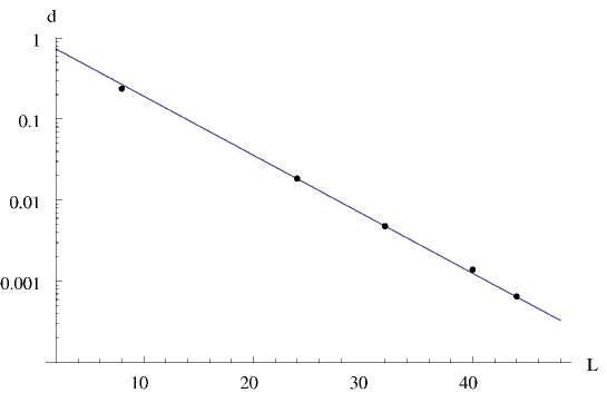
Figure 1: The average errors (dots) of the approximations to the 60 rotations of the icosahedral group with the brute-force search as a function of the length of the weaves used. These errors characterize the pseudogroups used in the hashing algorithm for the lengths $L=8$, 24, 32, 40, and 44. The results are in very good agreement with the prediction in Eq. (18) (solid line).

3.3 The Icosahedral group

The hashing procedure relies on the possibility of exploiting the group structure of a finite subgroup of the target space to build sets $\mathcal{S}(L)$ of fine rotations, distributed with smaller and smaller mean distances from the identity, that can be used to progressively correct a first approximation of a target gate $T$. Therefore, it is fundamental to search, for every target space of unitary operators, a suitable subgroup to build the sets $\mathcal{S}$. Among the different finite subgroups of SU(2) we considered the $SO(3)$ subgroups corresponding to the symmetry group of the icosahedron and of the cube, which have order 60 and 24, respectively. However, for practical purposes, we will refer in the following mainly to the icosahedral group because its implementation of the hashing algorithm, as we will describe below, is more efficient in terms of the final braid length.

The icosahedral rotation group ${\mathcal{I}}$ is the largest polyhedral subgroup of SU(2), excluding reflection. For this reason, it has been often used to replace the full SU(2) group for practical purposes, as for example in earlier Monte Carlo studies of SU(2) lattice gauge theories [25], and its structure can be exploited to build meshes that cover the whole SU(2) [26].

${\mathcal{I}}$ is composed by 60 rotations around the axes of symmetry of the icosahedron (platonic solid with twenty triangular faces) or of its dual polyhedron, the dodecahedron (regular solid with twelve pentagonal faces); there are six axes of the fifth order (corresponding to rotations with fixed vertices), ten of the third (corresponding to the triangular faces) and fifteen of the second (corresponding to the edges). Let us for convenience write ${\mathcal{I}}=\{g_{0},g_{1},...,g_{59}\}$, where $g_{0}=e$ is the identity element. In figure 2a the elements of the icosahedral group are represented inside the SU(2) sphere.

Because of the group structure, given any product of $n$ elements of a subgroup $g_{i_{1}}g_{i_{2}}\cdots g_{i_{n}}$ there always exists a group element $g_{i_{n+1}}=g_{i_{n}}^{-1}\cdots g_{i_{2}}^{-1}g_{i_{1}}^{-1}$ that is its inverse. In this way $g_{i_{1}}g_{i_{2}}\cdots g_{i_{n}}g_{i_{n+1}}=e$ and one can find $O^{n}$ different ways of obtaining the identity element, where $O$ is the order of the group (60 in the case of the icosahedral one). This is the key property we will use in order to create a dense mesh $\mathcal{S}$ of fine rotations distributed around the identity operator in the target space. To achieve this goal, however, we need to break the exact group structure and to exploit the errors given by a brute-force search approximation of the elements of the chosen subgroup.

3.4 Pseudogroup

The main idea in the realization of the mesh $\mathcal{S}$ is that, representing the 60 elements of the subgroup $\mathcal{I}$ with weaves of a given length $L$, we can control, due to the relation (18), the average distance (or error) between the exact rotations in $\mathcal{I}$ and their braid representations that constitute the set $\tilde{\mathcal{I}}(L)$ which we will refer to as a pseudogroup.

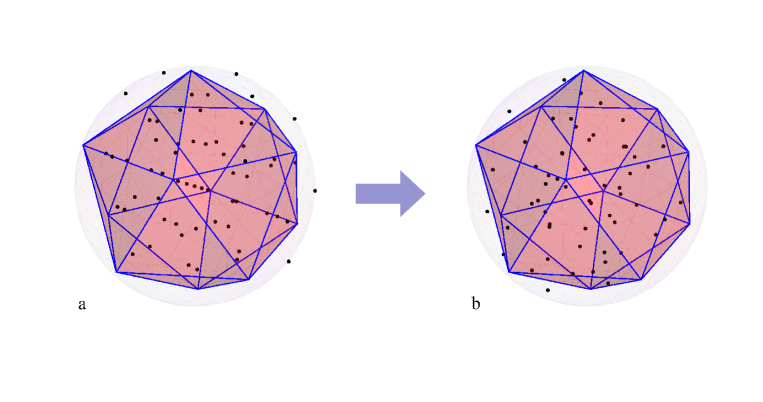
Figure 2: a: The icosahedral group representation inside the SU(2) sphere. b: the pseudogroup representation $\tilde{\mathcal{I}}(8)$ used in the preprocessor. Due to the large errors ($\sim 0.24$) the elements of $\tilde{\mathcal{I}}(8)$ seem to span the SU(2) sphere randomly.

Thanks to the homomorphism between SU(2) and $SO(3)$ we associate to every rotation $g\in\mathcal{I}$ a $2\times 2$ matrix (14). Then we apply a brute-force search of length $L$ to approximate the 60 elements in $\mathcal{I}$; in this way we obtain 60 braids that give rise to the pseudogroup $\tilde{\mathcal{I}}(L)=\{\tilde{g}_{0}(L),\tilde{g}_{1}(L),\dots,\tilde{g}_{59}(L)\}$. These braids are characterized by an average distance $\epsilon(L)$ with their corresponding elements $g_{i}\in\mathcal{I}$ given by Eq. (18). We notice from Fig. 2 that the large errors for $L=8$ completely spoil the symmetry of the group (and we will exploit this characteristic in the preprocessor of the hashing algorithm); however, increasing the length $L$, one obtains pseudogroups with smaller and smaller errors. Choosing, for instance, a fixed braid length of $L=24$, the error of each braid representation to its corresponding exact matrix representation varies from 0.003 to 0.094 with a mean distance of 0.018.

Therefore the braid representations of the icosahedral group with different lengths are obtained by a brute-force search once and for all. The so obtained braids are then stored for future utilizations and this is the only step in which we apply, preliminarily, a brute-force search. Due to limiting computing resources, we construct the pseudogroups representations for the 60 rotations up to the length $L=68$, which, as we will describe below, is sufficient to implement three iterations of the hashing algorithm. In principle one could calculate the brute-force approximation of the group elements to larger lengths once and for all, in order to use them for a greater number of iterations. The average errors characterizing the main pseudogroups we use in the iterations are shown in Fig. 1; they agree well with Eq. (18).

Let us stress that that the 60 elements of $\tilde{\mathcal{I}}(L)$ (for any finite $L$) do not close any longer the composition laws of the icosahedral group; in fact a pseudogroup $\tilde{\mathcal{G}}(L)$ becomes isomorphic to its corresponding group ${\mathcal{G}}$ only in the limit $L\rightarrow\infty$. If the composition law $g_{i}g_{j}=g_{k}$ holds in $\mathcal{I}$, the product of the corresponding elements $\tilde{g}_{i}(L)$ and $\tilde{g}_{j}(L)$ is not $\tilde{g}_{k}(L)$, although it can be very close to it for large enough $L$. Interestingly, the distance between the product $\tilde{g}_{i}(L)\,\tilde{g}_{j}(L)$ and the corresponding element $g_{k}$ of ${\mathcal{I}}$ can be linked to the Wigner-Dyson distribution (see Sec. 4.2).

Using the pseudogroup structure of $\tilde{\mathcal{I}}(L)$, it is easy to generate a mesh $\mathcal{S}(L)$ made of a large number of braids only in the vicinity of the identity matrix: this is a simple consequence of the original group algebra, in which the composition laws allow us to obtain the identity group element in various ways. The set $\mathcal{S}$ is instrumental to achieve an important goal, i.e. to search among the elements of $\mathcal{S}$ the best correction to apply to a previous approximation of the target single-qubit gate $T$ we want to hash.

It is important to notice that, changing the length $L$ of the pseudogroup representation, we can control the average distance of the fine rotations in $\mathcal{S}$ from the identity. To correct an approximation of $T$ with an error $\varepsilon$, we need a mesh $\mathcal{S}$ characterized by roughly the same average error in order to reach an optimal density of possible corrections and so increase the efficiency of the algorithm. Therefore, knowing the average error of the distribution of the approximations we want to improve, we can choose a suitable $L$ to generate a mesh. As represented in Fig. 3, this allows us to define a series of denser and denser meshes to iterate the hashing algorithm in order to correct at each step the expected mean error, which we have determined by analyzing the distributions of errors of 10000 random targets after the corresponding iteration.

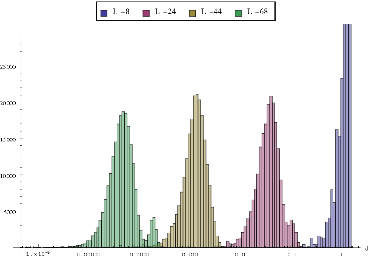
Figure 3: Distribution of the meshes $\mathcal{S}(L,3)$ used by the renormalization scheme of the hashing algorithm. The distance $d$ from the identity is represented in logarithmic scale. The mesh with $L=8$ comprehends every possible product of three elements in $\tilde{\mathcal{I}}(8)$ and, therefore, it spans the whole SU(2) space up to the distance $\sqrt{2}$. The meshes $\mathcal{S}(24,3)$, $\mathcal{S}(44,3)$ and $\mathcal{S}(68,3)$, instead, are the product of four braids whose corresponding rotations are combined to approximate the identity. $\mathcal{S}(24,3)$ and $\mathcal{S}(44,3)$ follow the Wigner-Dyson distribution while $\mathcal{S}(68,3)$ exhibits a second local maximum due to the incomplete brute-force search we used to obtain $\tilde{\mathcal{I}}(68)$.

To create the mesh of fine rotations, labeled by $\mathcal{S}(L,n)$, we consider all the possible ordered products $\tilde{g}_{i_{1}}(L)\tilde{g}_{i_{2}}(L)\dots\tilde{g}_{i_{n}}(L)$ of a fixed $n\geq 2$ elements of $\tilde{\mathcal{I}}(L)$ of length $L$ and multiply them by the matrix $\tilde{g}_{i_{n+1}}(L)\in\tilde{\mathcal{I}}(L)$ such that $g_{i_{n+1}}=g_{i_{n}}^{-1}\dots g_{i_{2}}^{-1}g_{i_{1}}^{-1}$. In this way we generate all the possible combinations of $n+1$ elements of ${\mathcal{I}}$ that produce the identity, but, thanks to the errors that characterize the braid representation $\tilde{\mathcal{I}}$, we obtain $60^{n}$ small rotations in SU(2), corresponding to braids of length $(n+1)L$. In Sec. 4.2 we will describe their distribution around the identity with the help of random matrices.

4 Itarative pseudogroup hashing in SU(2)

4.1 The iterative pseudogroup hashing algorithm

The hashing algorithm is based on the possibility of finding progressive corrections to minimize the error between the target gate $T\in SU(2)$ and the braids that represent it. These corrections are chosen among the meshes $\mathcal{S}(L_{i},3)$ whose distribution around the identity operator is shown in Fig. 3.

The algorithm consists of a first building block, called preprocessor, whose aim is to give an initial approximation $\tilde{T}_{0}$ of $T$, and a main processor composed of a series of iterations of the hashing procedure that, at each step, extend the previous representation by a braid in $\mathcal{S}(L_{i},3)$. The final braid has the form

$$\tilde{T}_{3}=\underbrace{\tilde{g}_{j_{1}}\left(L_{0}\right)\cdots\tilde{g}_{j_{3}}\left(L_{0}\right)}_{\rm Preprocessor}\underbrace{\tilde{g}_{p_{1}}\left(L_{1}\right)\cdots\tilde{g}_{p_{4}}\left(L_{1}\right)}_{\rm 1st\ Iteration}\underbrace{\tilde{g}_{q_{1}}\left(L_{2}\right)\cdots\tilde{g}_{q_{4}}\left(L_{2}\right)}_{\rm 2nd\ Iteration}\underbrace{\tilde{g}_{r_{1}}\left(L_{3}\right)\cdots\tilde{g}_{r_{4}}\left(L_{3}\right)}_{\rm 3rd\ Iteration}$$ (19)

Each $\tilde{g}_{j}(L_{i})$ is an element of the pseudogroup $\tilde{\mathcal{I}}\left(L_{i}\right)$ and, as explained in the previous section, the braid segment in each main iteration is constrained by $g_{k_{4}}=g_{k_{3}}^{-1}g_{k_{2}}^{-1}g_{k_{1}}^{-1}$, $k=p$, $q$, or $r$.

Each iteration starts from an input approximation $\tilde{T}_{i-1}$ with a distance $\varepsilon_{i-1}$ from the target $T$. We exploit the elements of the mesh $\mathcal{S}(L_{i},n)$ to generate a new braid $\tilde{T}_{i}$ with a smaller distance $\varepsilon_{i}$. The lengths $L_{i}$ in Eq. (19), which characterize the pseudogroups used in the main processor, control the density of the corresponding meshes and are chosen among the sets of stored pseudogroups in order to correct the residual error in an efficient way (see Sec. 5).

Let us analyze now the details of each step in the hashing algorithm. The preprocessor is a fast procedure to generate a rough approximation of the target gate $T\in SU(2)$ and, in general, it associates to every $T$ a braid which is an element of $[\tilde{\mathcal{I}}\left(L_{0}\right)]^{m}$ (of length $mL_{0}$). Therefore, the preprocessor approximates $T$ with the ordered product of elements in the icosahedral pseudogroup $\tilde{\mathcal{I}}\left(L_{0}\right)$ that best represents it, minimizing their distance. Thus we obtain a starting braid

$$\tilde{T}^{L_{0},m}_{0}=\tilde{g}_{j_{1}}\left(L_{0}\right)\tilde{g}_{j_{2}}\left(L_{0}\right)\dots\tilde{g}_{j_{m}}\left(L_{0}\right)$$ (20)

with an initial error to reduce. The preprocessor procedure relies on the fact that, choosing a small $L_{0}$, we obtain a substantial discrepancy between the elements $g_{i}$ of the icosahedral group and their representatives $\tilde{g}_{i}$, as shown in Fig. 2. Because of these seemingly random errors, the set $[\tilde{\mathcal{I}}(L_{0})]^{m}$ of all the products $\tilde{g}_{j_{1}}\tilde{g}_{j_{2}}\dots\tilde{g}_{j_{m}}$ is well spread all over SU(2) and can be thought as a random discretization of the group. In particular we find that the pseudogroup $\tilde{\mathcal{I}}(8)$ has an average error of about $0.24$ and it is sufficient to take $m=3$ [as we did in Eq. (19)] to cover the whole SU(2) in an efficient way with $60^{3}$ operators. The average error for an arbitrary single-qubit gate with its nearest element $\tilde{T}^{8,3}_{0}\in[\tilde{\mathcal{I}}(8)]^{3}$ is about 0.027.

One can then apply the main processor to the first approximation $\tilde{T}_{0}$ of the target gate. Each subsequent iteration improves the previous braid representation of $T$ by adding a finer rotation to correct the discrepancy with the target and generate a new braid. In the first iteration we use the mesh $\mathcal{S}(L_{1},n)$ to efficiently reduce the error in $\tilde{T}^{l,m}_{0}$. Multiplying $\tilde{T}^{l,m}_{0}$ by all the elements of $\mathcal{S}(L_{1},n)$, we generate $60^{n}$ ($O^{n}$ if we use a subgroup of order $O$) possible braid representations of $T$ :

$$\tilde{T}^{l,m}_{0}\tilde{g}_{i_{1}}\tilde{g}_{i_{2}}\dots\tilde{g}_{i_{n}}\tilde{g}_{i_{n+1}}$$ (21)

Among these braids of length $(n+1)L_{1}+mL_{0}$, we search the one with the shortest distance to the target gate $T$. This braid, $\tilde{T}_{1}\left(L_{0},m,L_{1},n\right)$, is the result of the first iteration in the main processor.

The choice of $L=24$ for the first step is dictated by the analysis of the mean error of the preprocessor ($\sim 0.03$) that requires, as we will see in the following section, a pseudogroup with compatible error for an efficient correction. An example of the first iteration is illustrated in Ref. [6].

With $\tilde{T}_{1}$ we can then apply the second and third iterations of the main processor to obtain an output braid of the form in Eq. (19). These iterations further reduce the residual discrepancy in decreasing error scales. Each step in the main processor requires the same runtime, during which a search within $60^{n}$ braids selects the one with the shortest distance to $T$. One must choose appropriate pseudogroups with longer braid lengths $L_{2}$ and $L_{3}$ to generate finer meshes. As for $L_{1}$, we choose $L_{2}$ and $L_{3}$ to match the error of the corresponding pseudogroup to the respective mean residual error. In practice, we choose $L_{2}=44$ and $L_{3}=68$. The final output assumes the form in Eq. (19) and the average distance to the target braid (in 10000 random tests) is $2.29\times 10^{-5}$ after the second iteration and $8.24\times 10^{-7}$ after the third. Without reduction the final length is 568; however, due to shortenings at the junctions where different braid segments meet, the practical final length of the weave is usually smaller.

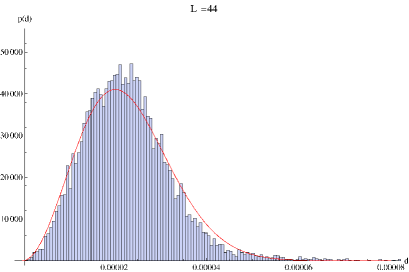
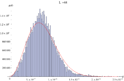
Figure 4: Probability densities of the distance $d$ from the target of 10000 random tests after the second ($L=44$) and third ($L=68$) main processors. The trend agrees with the unitary Wigner-Dyson distribution with average errors $2.28\times 10^{-5}$ and $7.60\times 10^{-7}$, respectively.

4.2 Connection with random matrix theory and reduction factor for the main processor

To analyze the efficiency of the main processor we must study the random nature of the meshes $\mathcal{S}(L,n)$. The distribution of the distance between the identity and their elements has an intriguing connection to the Gaussian unitary ensemble of random matrices, which helps us to understand how close we can approach the identity in this way, and therefore what the optimal choice of the lengths of the pseudogroups is for each iteration of the main processor.

Let us analyze the group property deviation for the pseudogroup $\tilde{\mathcal{I}}(L)$ for braids of length $L$. One can write $\tilde{g}_{i}=g_{i}\mathrm{e}^{i\Delta_{i}}$, where $\Delta_{i}$ is a Hermitian matrix, indicating the small deviation of the finite braid representation to the corresponding SU(2) representation for an individual element. For a product of $\tilde{g}_{i}$ that approximate $g_{i}g_{j}\cdots g_{n+1}=e$, one has

$$\tilde{g}_{i}\tilde{g}_{j}\cdots\tilde{g}_{n+1}=g_{i}\mathrm{e}^{i\Delta_{i}}g_{j}\mathrm{e}^{j\Delta_{j}}\cdots g_{n+1}\mathrm{e}^{i\Delta_{n+1}}=\mathrm{e}^{iH_{n}},$$ (22)

where $H_{n}$, related to the accumulated deviation, is

$$H_{n}=g_{i}\Delta_{i}g_{i}^{-1}+g_{i}g_{j}\Delta_{j}g_{j}^{-1}g_{i}^{-1}+\cdots+g_{i}g_{j}\cdots g_{n}\Delta_{n}g_{n}^{-1}\cdots g_{j}^{-1}g_{i}^{-1}+\Delta_{n+1}+O(\Delta^{2}).$$ (23)

The natural conjecture is that, for a long enough sequence of matrix product, the Hermitian matrix $H_{n}$ tends to a random matrix corresponding to the Gaussian unitary ensemble. This is plausible as $H_{n}$ is a Hermitian matrix that is the sum of random initial deviation matrices with random unitary transformations. A direct consequence is that the distribution of the eigenvalue spacing $s$ obeys the Wigner-Dyson form [28],

$$P(s)={\frac{32}{\pi^{2}s_{0}}}\left({\frac{s}{s_{0}}}\right)^{2}\mathrm{e}^{-(4/\pi)(s/s_{0})^{2}},$$ (24)

where $s_{0}$ is the mean level spacing. For small enough deviations, the distance of $H_{n}$ to the identity, $d\left(1,\mathrm{e}^{iH_{n}}\right)=\|H_{n}\|+O\left(\|H_{n}\|^{3}\right)$, is proportional to the eigenvalue spacing of $H$ and, therefore, should obey the same Wigner-Dyson distribution. The conjecture above is indeed well supported by our numerical analysis, even for $n$ as small as 3 or 4: the distances characterizing the meshes with $L=24$ and $L=48$ obtained from the corresponding pseudogroups (Fig. 3) follow the unitary Wigner-Dyson distribution.

The elements of the meshes $\mathcal{S}(L,n)$ are of the form in Eq. (22) and this implies that, once we choose a pseudogroup $\tilde{\mathcal{I}}(L)$ whose average error $\bar{d}(L)$ is given by Eq. (18), the mean distance $s_{0}$ in (24) of the corresponding mesh from the identity is $s_{0}(L)\approx\sqrt{n+1}\,\bar{d}(L)$ as resulting from the sum of $n+1$ gaussian terms.

At each iteration of the main processor, we increase the braid by $(n+1)=4$ braid segments with length $L_{i}$. By doing that, we create $60^{n}$ braids and the main processor search, among them, the best approximation of the target. Therefore, the runtime is linear in the dimension of the meshes used and in the number of iterations. The unitary random matrix distribution implies that the mean deviation of the 4-segment braids from the identity (or any other in its vicinity) is a factor of $\sqrt{n+1}$ times larger than that of an individual segment. Considering the 3-dimensional nature of the unitary matrix space, we find that at each iteration the error (of the final braid to the target gate) is reduced, on average, by a factor of $f\sim 60^{n/3}/\sqrt{n+1}=30$, where 60 is the number of elements in the icosahedral group. This has been confirmed in the numerical implementation.

4.3 Hashing with the cubic group

For comparison, we also implemented the hashing procedure with the smaller cubic group. In this case the rotations in the group of the cube are 24; thus we choose $n=4$ to generate a comparable number of elements in each mesh $\mathcal{S}(L,n)$. Our implementation of the hashing with the cubic group uses a preprocessor with $L_{0}=8$ and $m=4$ and a main processor with $L_{1}=24$ and $n=4$. Approximating over 100 random targets, we obtained an average error $6.92\times 10^{-4}$ after the main processor, comparable to $7.24\times 10^{-4}$ after the first iteration in the previous icosahedral group implementation. This result is consistent with the new reduction factor $f_{\rm cube}=24^{4/3}/\sqrt{5}\approx 30.96$. However we note that the cubic hashing is less efficient both in terms of the braid length (because it requires $n=4$ instead of $n=3$) and in terms of the runtime (because the time required for the searching algorithm is linear in the elements of $\mathcal{S}$ and $24^{4}>60^{3}$).

4.4 Tail correction

The choice of the proper $L_{i}$ is important. We determine them by the average error before each iteration. If a certain $L_{i}$ is too large, it generates a mesh around the identity that may be too small to correct the error relatively far from the identity, where the mesh is very fine. On the other hand, if $L_{i}$ is too small, the mesh may be too sparse to correct efficiently. The former situation occurs exactly when we treat the braids with errors significantly larger than the average; they correspond to the rare events in the tail of the distributions as shown in Fig. 4. Such an already large error is then amplified with the fixed selection of $L_{i}=24$, 44, and 68. To avoid this, one can correct the “rare” braids $\tilde{T}_{i-1}$, whose error is higher than a certain threshold, with a broader mesh [e.g., $\mathcal{S}(L_{i}-4,n)$].

The tail correction is very efficient. If we correct for the $0.6\%$ of the targets with the largest errors in the second iteration with $\mathcal{S}(40,3)$ instead of $\mathcal{S}(44,3)$, we reduce the average error by about $8\%$ after the third iteration (see Table 1). The drastic improvement is due to the fact that once a braid is not properly corrected in the second iteration, the third one becomes ineffective. We can illustrate this situation with the example of the operator $iY$ (where $Y$ is the Pauli matrix): without tail correction it is approximated in the first iteration with an error of $0.0039$, which is more than 5 times the average error expected. After the second iteration, we obtain an error of $4.3\times 10^{-4}$ (almost 20 times higher than the average value) and after the third the error becomes $2.0\times 10^{-4}$ (more than 200 times the mean value). If we use $\mathcal{S}(40,3)$ instead of $\mathcal{S}(44,3)$ in the second iteration we obtain an error $4.46\times 10^{-5}$, with a shorter braid than before, and a final error of $1.31\times 10^{-6}$ which is less than twice the average error.

	Without tail correction		With tail correction
10000 trials	Average Error	$\sigma$	Average Error	$\sigma$
Preprocessor*	$0.027$	$0.010$	$0.027$	$0.010$
Main, 1st iteration*	$7.24\times 10^{-4}$	$3.36\times 10^{-4}$	$7.24\times 10^{-4}$	$3.36\times 10^{-4}$
Main, 2nd iteration	$2.29\times 10^{-5}$	$1.3\times 10^{-5}$	$2.28\times 10^{-5}$	$9.79\times 10^{-6}$
Main, 3rd iteration	$8.24\times 10^{-7}$	$5.6\times 10^{-6}$	$7.60\times 10^{-7}$	$3.27\times 10^{-7}$

Table 1: Average error and standard deviation for the hashing algorithm after the preprocessor and the three iterations of the main processor. The outputs in absence or presence of a tail correction for the second and third iterations are shown (the asterisk indicates that the preprocessor and the first iteration are not affected by the tail correction). This correction is based on the psudogroups with length 40 and 64 instead of the standard ones, 44 and 68. Only about the $0.6\%$ of the targets used the tail correction in the second iteration, but one notice that the results, both in terms of average error and in terms of standard deviation $\sigma$, are extremely affected by these rare events.

5 General efficiency of the algorithm

To evaluate the efficiency of the hashing algorithm it is useful to calculate the behaviour of the maximum length of the braids and of the runtime with respect to the average error obtained. We compare the results with those of the brute-force search (which gives the optimal braid length) and of the Solovay-Kitaev algorithm.

As described in Sec. 4.2, we reduce the average error at the $i$th iteration to

$$\varepsilon_{i}\sim\varepsilon_{i-1}/f\qquad{\rm with}\quad f\approx 30.$$ (25)

The total number of iterations (or depth) to achieve a final error of $\varepsilon$ is then

$$M\sim\frac{\ln(1/\varepsilon)}{\ln{f}},$$ (26)

so the expected error after each iteration is

$$\ln(1/\varepsilon_{i})\sim i\ln f.$$ (27)

For efficient optimization, we choose the length $L_{i}$ of the braid segments at the $i$th iteration to approximate the corresponding icosahedral group elements with an average error of $\varepsilon_{i-1}$ (see discussions in Sec. 4.4). So we have, from Eq. (18),

$$L_{i}\sim\mathcal{L}\ln\left({1/\varepsilon_{i-1}}\right)$$ (28)

with $\mathcal{L}\approx 6$ [see Eq. (18)] and the length of the braid we construct increases by $(n+1)L_{i}=4L_{i}$ at the $i$-th iteration, i.e.,

$$L_{i}-L_{i-1}=4\mathcal{L}\ln\left({1/\varepsilon_{i-1}}\right)\sim 4\mathcal{L}(i-1)\ln f.$$ (29)

Thus the total length of the braid with an error of $\varepsilon$ is

$$L_{M}\sim\sum_{i=1}^{M}4\mathcal{L}(i-1)\ln{f}\sim M^{2}.$$ (30)

The final results for the hashing algorithm are, therefore,

$$L_{\rm qh}\sim\left(\ln\left(1/\varepsilon\right)\right)^{2},$$ (31)

$$T_{\rm qh}\sim M\sim\ln\left(1/\varepsilon\right).$$ (32)

We have explicitly confirmed that we can realize the perfect length-error scaling as shown in Fig. 5 up to three iterations in the main processor.

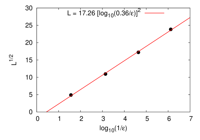
Figure 5: The scaling performance of the hashing algorithm in terms of the square root of the maximum length versus the logarithm of the inverse error. The error is the average error in approximating 10000 random targets after the preprocessor and the three iterations in the main processor. The results agree with the expected behaviour [Eqs. (31) and (32)].

We can conclude that while no method beats the brute-force search in length, we achieve a respectable gain in time. Comparing these results with the length of the braids obtained by the Solovay-Kitaev algorithm in Eq. (3) and with its runtime in Eq. (4), the hashing algorithm gives results that are better than the Solovay-Kitaev results in terms of length and significantly better in terms of time.

6 Conclusions

We have demonstrated, for a generic universal topological quantum computer, that the iterative pseudogroup hashing algorithm allows an efficient search for a braid sequence that approximates an arbitrary given single-qubit gate. This can be generalized to the search for two-qubit gates as well. The algorithm applies to the quantum gate construction in a conventional quantum computer given a small universal gate set, or any other problems that involve realizing an arbitrary unitary rotation approximately by a sequence of “elementary” rotations.

The algorithm uses a set of pseudogroups based on the icosahedral group or other finite subgroups of SU(2), whose multiplication tables help generate, in a controllable fashion, smaller and smaller unitary rotations, which gradually (exponentially) reduce the distance between the result and the target. The iteration is in the same spirit as a generic renormalization group approach, which guarantees that the runtime of the algorithm is proportional to the logarithm of the inverse average final error $1/\varepsilon$; the total length of the braid is instead quadratic in $\ln(1/\varepsilon)$, and both the results are better than the Solovay-Kitaev algorithm introduced in textbooks.

We have explicitly demonstrated that the result from the performance analysis is in excellent agreement with that from our computer simulation. We also showed that the residual error distributes according to the Wigner-Dyson unitary ensemble of random matrices. The connection of the error distribution to random matrix theory ensures that we can efficiently carry out the algorithm and improve the rare cases in the distribution tail.

The overhead of the algorithm is that we need to prepare several sets of braid representations of the finite subgroup elements. Obtaining the longer representation can be time-consuming; but fortunately, we only need to compute them once and use the same sets of representations for all future searches.

7 Acknowledgements

This work is supported by INSTANS (from ESF), 2007JHLPEZ (from MIUR), and the 973 Program under Project No. 2009CB929100. X. W. acknowledges the Max Planck Society and the Korea Ministry of Education, Science and Technology for the support of the Independent Junior Research Group at the APCTP. M. B. and G. M. are grateful to the APCTP for the hospitality in Pohang where part of this study was carried out.

Appendix A Distribution of the best approximation in a given set of braids

In this Appendix we derive the distribution of the approximation to a gate in a given set of $N$ braids in the vicinity of the identity. While it is sufficient for the discussions in the main text, this derivation can be generalized to the more generic cases. Let us assume that the targeted gate is $g_{0}=U(\hat{l},\phi_{0})$ as defined in Eq. (14). The distance between $g_{0}$ and the identity is $s_{0}=2\sin(\phi_{0}/4)\approx\phi_{0}/2$ for small $\phi_{0}$. We then search in a given set of braids, either with a distribution as given in Eq. (17) or from a generated random matrix distribution as discussed in Sec. 4.2, the one with the shortest distance to the target.

We consider an arbitrary braid with representation $g=U\left(\hat{m},\phi\right)$ in a collection with a distribution $p(s)$ of the distance to the identity $s=2\sin(\phi/4)$. We define

$$P(x)=\int_{0}^{x}p(s)ds,$$ (33)

which is the probability of having a distance less than $x\leq\sqrt{2}$. Obviously $P(x)$ is a monotonically increasing function bound by $P(0)=0$ and $P(\sqrt{2})=1$. The distance $d(g_{0},g)$ between $g$ and $g_{0}$ is the same as that between $g_{0}^{-1}g$ and the identity. To the first order in $\phi$ and $\phi_{0}$ (as we assume all braids/gates are in the vicinity of the identity braid) we have, from Eq. (16)

$$d(g_{0},g)\approx\sqrt{s^{2}+s_{0}^{2}-2(\hat{l}\cdot\hat{m})s_{0}s}=\left|\left|s\hat{m}-s_{0}\hat{l}\right|\right|,$$ (34)

which is bound by $s+s_{0}$ and $|s-s_{0}|$. We can see that the chance to find a braid that is close to $g_{0}$ is large when $p(s)$ peaks around $s_{0}$. If we denote the probability of having no braids within a distance of $t$ by $Q(t)$, the probability of having the braid with the shortest distance between $t$ and $t+dt$ is

$$Q(t)-Q(t+dt)=Q(t)\left\langle Ndt\int_{0}^{\sqrt{2}}p(s)ds\delta\left(t-d(g_{0},g)\right)\right\rangle,$$ (35)

where the angled bracket implying the angular average of the averaged number of braids with a distance between $t$ and $t+dt$. Therefore,

$$-\frac{d\ln Q(t)}{dt}=N\left\langle\int_{0}^{\sqrt{2}}p(s)ds\delta\left(t-d(g_{0},g)\right)\right\rangle.$$ (36)

As an example, we consider $s_{0}=0$ [i.e., with the full SU(2) rotation symmetry of the distribution], in which case

$$-\ln Q(t)=N\int_{0}^{t}p(s)ds=NP(t),$$ (37)

or $Q(t)=\exp[-NP(t)]$. $NP(t)$ is the expected number of braids with a distance to the identity less than $t$. The differential probability of having the braid with the nearest distance between $t$ and $t+dt$ is, therefore,

$$q(t)\equiv-{\frac{dQ(t)}{dt}}=N{dP(t)\over dt}e^{-NP(t)}=Np(t)e^{-NP(t)}.$$ (38)

Combining the results with Eq. (17), we estimate for the brute-force search

$$q_{BF}(t;L)=N(L)p_{BF}(t)e^{-N(L)P_{BF}(t)}$$ (39)

with an average distance

$$\bar{d}(L)=\frac{\pi^{1/3}\left[\Gamma\left(\frac{1}{3}\right)-\Gamma\left(\frac{1}{3},\frac{8\sqrt{2}N(L)}{3\pi}\right)\right]}{6^{2/3}[N(L)]^{1/3}}$$ (40)

where $\Gamma(a,x)$ is the incomplete gamma function

$$\Gamma(a,x)=\int_{x}^{\infty}dtt^{a-1}e^{-t}.$$ (41)

In the large $L$ limit, $\bar{d}(L)\approx 1.021e^{-L/5.970}$. This is the result we quoted in Eq. (18).

References

References

- [1] M. A. Nielsen and I. L. Chuang, Quantum Computation and Quantum Information, Cambridge University Press (2000), Chap. 4.
- [2] D. P. DiVincenzo, Phys. Rev. A, 51 1015, (1995).
- [3] A. Yu. Kitaev, A. H. Shen, and M. N. Vyalyi, Classical and Quantum Computation, Am. Math. Soc. (2002), Sec. 8.
- [4] C. M. Dawson and M. A. Nielsen, Quant. Info. Comp. 6, 81 (2006).
- [5] L. Hormozi et al., Phys. Rev. B 75, 165310 (2007).
- [6] M. Burrello et al., Phys. Rev. Lett. 104 160502 (2010).
- [7] A. Yu. Kitaev, Ann. Phys. 303, 2 (2003);
- [8] M. Freedman, M. Larsen, and Z. Wang, Commun. Math. Phys. 227, 605 (2002); 228, 177 (2002); M. Freedman, A. Kitaev, and Z. Wang, ibid. 227, 587 (2002).
- [9] C. Nayak et al., Rev. Mod. Phys. 80, 1083 (2008).
- [10] G. K. Brennen and J. K. Pachos, Proc. R. Soc. A, 464, 1 (2008).
- [11] J. Preskill, Lecture Notes on Topological Quantum Computation; available online at www.theory.caltech.edu/preskill/ph219/topological.pdf.
- [12] A. Stern, Ann. Phys. 323, 1 (2008).
- [13] N. R. Cooper, N. K. Wilkin, J. M. F. Gunn, Phys. Rev. Lett. 87, 120405 (2001).
- [14] N. Read and D. Green, Phys. Rev. B 61, 10267 (2000).
- [15] P. Bonderson et al., arXiv:1003.2856 (2010).
- [16] N. E. Bonesteel et al., Phys. Rev. Lett. 95, 140503 (2005).
- [17] S. H. Simon et al., Phys. Rev. Lett. 96, 070503 (2006).
- [18] H. Xu and X. Wan, Phys. Rev. A 78, 042325 (2008).
- [19] M. Baraban, N. E. Bonesteel, and S. H. Simon, Phys. Rev. A 81, 062317 (2010).
- [20] N. Read and E. H. Rezayi, Phys. Rev. B 59, 8084 (1999).
- [21] J. S. Xia, et al., Phys. Rev. Lett. 93, 176809 (2004).
- [22] E. Ardonne and K. Schoutens, Phys. Rev. Lett. 82, 5096 (1999); E. Ardonne et al., Nucl. Phys. B 607, 549 (2001); E. Ardonne and K. Schoutens, Ann. Phys. 322, 201 (2007).
- [23] A. Yu. Kitaev, Ann. Phys. 321, 2 (2006).
- [24] H. Xu and X. Wan, Phys. Rev. A 80, 012306 (2009).
- [25] C. Rebbi, Phys. Rev. D 21, 3350 (1980); D. Petcher and D. H. Weingarten, Phys. Rev. D 22, 2465 (1980); G. Bhanot, K. Bitar, and R. Salvador, Phys. Lett. B 188, 246 (1987).
- [26] R. Mosseri, J. Phys. A: Math. Theor. 41, 175302 (2008).
- [27] Object-oriented source codes available for download at http://sites.google.com/site/braidanyons/.
- [28] M. Mehta, Random Matrices, 2nd ed. (Academic, San Diego, 1991).