Density quantization method in the optimal portfolio choice with partial observation of stochastic volatility

Abstract

Computational aspects of the optimal consumption and investment with the partially observed stochastic volatility of the asset prices are considered. The new quantization approach to filtering – density quantization – is introduced which reduces the original infinite dimensional state space of the problem to the finite quantization set. The density quantization is embedded into the numerical algorithm to solve the dynamic programming equation related to the portfolio optimization.

1 Introduction

The optimal investment portfolio and consumption path choice have been studied extensively for about 5 decades but still poses computational difficulties. The standard Merton-like investment problem evolved into many research fields and one of them are the partial observation models studied by Lakner [15], Pham and Quenez [19], Sass and Haussmann [21], Stettner [24], Baghery and Øksendal [1], Hałaj [13], Brendle [6]. Those models are imbedded into the control theory framework with partial information [4]. In the case of portfolio choice in the partial observation, the investor does not observe all the factors defining the dynamics of the market. Hence, the optimal strategies are not only functions of the state variables like the wealth of the investor, but depend on investor’s beliefs about the true value of asset prices and economic factors [24]. Those beliefs are represented by the probability distribution of values of the factors given available information on the market. This makes the value function of the investor to be defined on the infinite dimensional state space. Following the quantization approach we introduced the numerical method to solve the related dynamic programming equation.

The partial observation shows up in the portfolio models in two forms. The first one is related to trend parameters of assets prices, the second one to volatility. Models with an unobserved trend are usually easy to reformulate in a full observation setting (eg. by the change of measure approach the drift parameter of diffusion price processes vanish). The portfolio problems with unknown volatility are, however, more realistic and we assumed in our model that the volatility of stocks is unobserved, also driven by some unobserved economic factors. This is a standard assumption in advanced models of volatility [2, 12].

We consider the numerical approximation of the solution to the following consumption and investment problem. For clarity of the presentation of the main idea we postpone the rigorous assumptions to the section 1.2. Let us denote by $\mathbb{T}$ the set $\{0,1,\dots,T\}\subset\mathbb{N}\cap\{0\}$. We consider the probability space $(\Omega,\mathcal{F},\mathbf{P})$ and the discrete filtration $\mathbb{F}\colon\!\!=\{\mathcal{F}_{t}\}_{{t\in\mathbb{T}}}$. On $\mathcal{F}$ we define $N$ sequences of the IID random variables $\{\epsilon_{i}(t)\}_{t\in\mathbb{T}}$, $i\in\{1,\dots,N\}$, each of which has a positive density $\phi$. By $\{r(t)\}_{t\in\mathbb{T}}$ we denote a process of the interest rates in the economy, constant within the periods $[t,\,t+1]$ and by $\{S_{0}(t)\}_{t\in\mathbb{T}}$ we denote the bank account process given by the recurrence $S_{0}(0)=1$ and $\forall n>0\,S_{0}(t+1)=(1+r(t))S_{0}(t)$.

We assume that the process of the economic factors measuring the economic situation is denoted by $\{Y(t)\}_{t\in\mathbb{T}}$ and given by the following equation:

$$Y(0)=y_{0}\qquad Y(t+1)=Y(t)+\alpha\left(\bar{y}-Y(t)\right)+\sigma_{Y}\xi(t+1),$$ (1)

where $(\xi(t))_{t\in\mathbb{T}}$ is the IID sequence of $K$-dimensional random variables, each with positive density $\psi$. $\sigma_{Y}$ is the full-rank $K\times K$ matrix. The tradable assets on the market have the following dynamics for $i\in\{1,\dots,N\}$:

$$S_{i}(t+1)=S_{i}(t)\exp\left(\mu(Y(t+1))+\sigma(Y(t+1))\epsilon_{i}(t+1)\right).$$ (2)

There are two types of shocks on the market: the idiosyncratic $\epsilon$ which are asset (eg. company) specific and the systemic $\xi$ which influence all the risky assets on the market.

The investor (and consumer at the same time) have preferences characterized by utility functions $u\colon\mathbb{R}^{K}\times\mathbb{R}_{+}\to\mathbb{R}$ and $u_{T}\colon\mathbb{R}^{K}\times\mathbb{R}_{+}\to\mathbb{R}$.

The return from investment in the asset $S_{i}$ in $t$ for $[t,t+1]$ is denoted by $R_{i}(t+1)={S_{i}(t+1)\over S_{i}(t)}$. The logarithmic return is denoted $R_{i}^{l}(t)=\ln(R_{i}(t))$. The wealth of the investor starting with capital $x_{0}$ and investing $\pi\colon\!\!=\{\pi(t)|t\in\mathbb{T}\}$ and consuming $c\colon\!\!=\{c(t)|t\in\mathbb{T}\}$ is defined by:

$$X(t+1)=\sum_{i=1}^{N}\pi_{i}(t){S_{i}(t+1)\over S_{i}(t)}+(X(t)-\sum_{i=1}^{N}\pi_{i}(t)-c(t))(1+r(t)),\quad X(0)=x_{0}.$$ (3)

The investor observes only the prices $S_{i}$ of the securities so his information is described by filtration $\mathbb{F}^{S}=\{\mathcal{F}^{S}_{t}\}_{{t\in\mathbb{T}}}$ where $\mathcal{F}^{S}_{t}\colon\!\!=\sigma(\{S_{i}(s)|i\in\{1,\dots,N\},\,s\leq t\})$. It is equivalent to observing $\mathbb{F}^{lR}\colon\!\!=\sigma(\{R_{i}^{l}(s)|i\in\{1,\dots,N\},\,s\leq t\})$ generated by log-returns from investment in $S$ which is more convenient for our purpose. The investor wants to optimize his utility from consumption and his terminal wealth. She maximizes the functional $J\colon\mathcal{A}(x)\to\mathbb{R}$ given by:

$$J(c,\pi)=\mathbf{E}\left\{\sum_{t=1}^{T-1}\delta^{t}u(c(t))+\delta^{T}u_{T}(Y(T),X^{c,\pi}(T))\right\},$$ (4)

where $T$ is the time horizon and $\mathcal{A}(x)$ is the set of the admissible controls $(c,\,\pi)$

$$\mathcal{A}(x)=\Big{\{}((c(0),\dots,c(T-1)),(\pi(0),\dots,\pi(T-1))|$$

$$(c(t),\pi(t))-\mathcal{F}^{lR}_{t}\mathrm{\!-\!measurable};\qquad 0\leq c(t)\leq X^{c,\pi}(t);$$

$$\sum_{i=1}^{N}\pi_{i}(t)\leq X^{c,\pi}(t)-c(t)\Big{\}}.$$

The solution maximizing $J$ is given by the special form of dynamic programming.

$$V(t,x,\varrho) = \sup_{\mathcal{A}(x)}\Bigg{\{}u(\bar{c})+\delta\mathbf{E}V\Big{(}t+1,x(\hat{R}^{l}(t+1)),\varrho_{t+1}(t+1,\hat{R}^{l}(t+1))\Big{)}\Bigg{\}}$$

The arguments $t$ and $x$ refer to usual time and current wealth state space variables (like in Bertsekas [5]). The variable $\rho$ measures the distribution of a random variable which is precisely defined in section 2 and corresponds to the process $Y$. Unlike in the full observation stochastic control in which case the value function at time $t$ depends on the realization of $Y(t)$, the partial observation allows the investor to assess only the most likely value of $Y(t)$ given the history of the asset prices. That is the intuition behind the dependence of $V$ on the whole distribution of $Y$ given $\mathcal{F}^{S}_{t}$.

The lack of closed form solutions to consumption/investment problems gives rise to research on numerical simulation methods to be applied to models with partial observation. The numerical procedure has to be designed in a special way to account for the natural high complexity of the state space of stochastic control. The literature does not give many examples of approximate solutions to the stochastic control with filtering. Runggaldier and Stettner [20] discretize transition probabilities and Desai et al. [10] proposed a particle filtering method to discretize a dynamic programming equation. There are numerous studies of numerical methods of filtering equations themselves. The Zakai equations which describe densities of unobserved parameters evolving in time as new information arrives to the market can be solved by means of the so-called particle filter methods [9]. Filter equations in discrete time can be estimated with the so-called quantization [16, 17, 18]. In the related paper Corsi et al. [8] also proposed the scheme to solve the dynamic programming equation of the partially observed control problem applying markovian quantization and approximated the given Markov Chain by the transition probability matrix. In this way, infinite dimensional random variables can be approximated by a finite set of point in an optimal way. We modified the standard quantization techniques to develop a different approach – density quantization – and we applied it to our control problem. Basically, the main idea is to find the optimal quantization set directly in the set of the unnormalized densities of the filter. In other words, the density quantization set is the set of the appropriately selected unnormalized density functions. It proved to be successful in recursively solving the dynamic programming equation.

The paper is organized as follows: First, we present the mathematical model of the market and decision making. Second, we show the influence partial information can exert on consumption of an investor in a simplistic theoretical example. Third, we rewrite the partially observed problem in a full observation setting, applying the change of measure approach and we solve it using the dynamic programming. Fourth, we define the density quantization and we show how the investment/consumption problem can be solved numerically. Finally, we illustrate the application of the developed numerical method in the example of the market model.

1.1 Notation

• $\mathcal{M}^{n\times m}$ — the set of matrices $M$ with $n$ rows and $m$ columns.

• $B^{n}(\mathcal{F})$ — the set of Borel functions $f\colon\Omega\times\mathbb{R}^{K}\to\mathbb{R}$, $f(\omega,\cdot)\in L^{n}(\mathbb{R}^{K})$.

• $\phi_{\mu,\sigma}(x)$ — Gaussian density i.e.

  $$\phi_{\mu,\sigma}(x)={1\over(2\pi)^{N/2}(\det(\Sigma))^{1/2}}\exp(-{1\over 2}(x-\mu)^{T}\Sigma^{-1}(x-\mu)),$$

  where $\mu$ is mean and $\Sigma\colon\!\!=\sigma\sigma^{\top}$ is covariance matrix.

• $\mathrm{vol}(A)$ — volume of a set $A\in\mathbb{R}^{n}$.

• $\mathrm{diam}(A)=\sup_{(x,y)\in A\times A}(\sum_{1\leq i\leq n}|x_{i}-y_{i}|^{2})^{1/2}$.

• $A^{c}$ — completion of set $A$.

1.2 Main technical assumptions

To show convergence of solutions of approximate problem to the original one we need 3 assumptions for $\phi$ and $\psi$.
[A0] $\sigma(\cdot)$ is bounded from 0, i.e. $\exists\sigma_{\mathrm{min}}>0$ such that $\forall y\in\mathbb{R}^{K}$ $\sigma(y)>\sigma_{\mathrm{min}}$.
[A1] $u$ and $u_{T}$ satisfy $\int_{\mathbb{R}^{N}\times\mathbb{R}^{K}}(\phi(x)+\psi(y))(u(\exp(x))+u_{T}(\exp(x),y))\mathrm{d}x\mathrm{d}y<\infty$.
[A2] For every $y\in\mathbb{R}^{N}$ and $a<1$, $\int_{\mathbb{R}^{K}}\phi({z-y\over a}){1\over\phi(y)}\mathrm{d}z<L_{\Phi}$.

[A0] and [A2] are necessary to show convergence of the numerical scheme. [A1] guarantees the integrability in the dynamic programming equations.

2 Filtering

The most fundamental task to be done before applying the standard dynamic programming toolkit to our consumption/investment selection is to transform the problem into the complete observation one. We apply changing of reference measure techniques similarly to Krishnamurthy and Le Gland [14], Elliot and Miao [12], Stettner [24]. After that, in the section 3, we transform the classical dynamic programming equation to make it suitable for our portfolio problem.

For each $t\in\mathbb{T}$ we define a random variable

$$\lambda_{t}={\phi\left(\sigma^{-1}(Y(t))[R^{(l)}(t)-\mu(Y(t))]\right)\over\det(\sigma(Y(t)))\phi(R^{(l)}(t))}{\psi\Big{(}\sigma_{Y}^{-1}[Y(t)-Y(t-1)-\alpha(\bar{y}-Y(t-1))]\Big{)}\over\det(\sigma_{Y})\psi(Y(t))}.$$

Let us construct a process $\Lambda$ in the following way: $\Lambda_{t}\colon\!\!=\prod_{s=1}^{t}\lambda_{s}.$

The process $\Lambda$ defines a new measure – the reference measure $\bar{\mathbf{P}}$. Let us define the filtration $\mathbb{F}^{lR,Y}\colon\sigma(\{R^{l}(s),Y(s)|i\in\{1,\dots,N\},\,s\leq t\})$. For each $t\in\mathbb{T}$, its restriction to $\mathcal{F}^{lR,Y}_{t}$ is defined:

$${\mathrm{d}\mathbf{P}\over\mathrm{d}\bar{\mathbf{P}}}\Big{|}_{\mathcal{F}^{lR,Y}_{t}}=\Lambda_{t}.$$

To study properties of stochastic processes under $\bar{\mathbf{P}}$ we extensively use the generalized Bayes formula: for $(\mathcal{F},\mathbf{P})$-measurable $Z$

$$\bar{\mathbf{E}}\left.\left[Z\right|\mathcal{F}^{Y}_{t}\right]={\mathbf{E}\left.\left[\Lambda^{-1}_{t}Z\right|\mathcal{F}^{Y}_{t}\right]\over\mathbf{E}\left.\left[\Lambda^{-1}_{t}\right|\mathcal{F}^{Y}_{t}\right]}\quad\mathrm{and}\quad\mathbf{E}\left.\left[Z\right|\mathcal{F}^{Y}_{t}\right]={\bar{\mathbf{E}}\left.\left[\Lambda_{t}Z\right|\mathcal{F}^{Y}_{t}\right]\over\bar{\mathbf{E}}\left.\left[\Lambda_{t}\right|\mathcal{F}^{Y}_{t}\right]}.$$ (5)

We assume that there exists a function-valued process $\varrho\colon\Omega\times\mathbb{T}\times\mathbb{R}^{K}\to L^{2}(\mathbb{R})$ satisfying for a $L^{2}$ Borel function $f$ we have

$$\bar{\mathbf{E}}\left.\left[\Lambda_{t}f(Y)\right|\mathcal{F}^{lR}_{t}\right]=\int_{\mathbb{R}^{K}}f(z)\varrho_{t}(z)\mathrm{d}z,\ t\in\mathbb{T}.$$ (6)

For a given $t$ the object $\varrho_{t}$ is the conditional unnormalized density of $Y$. We look for the recursive equation for $\varrho$ which – combining with the Bayes formula 5 – would give the tractable expression for filters used in the optimization. It makes the numerical simulation of the optimal consumption/investment strategies easier.

The main result of the section, relying on independence of $Y$ and $R^{l}$ under $\bar{\mathbf{P}}$ is given in the following theorem.

Theorem 2.1

Let us denote

$$\Phi(z,R^{l}(t)) \colon\!\!= {\phi\Big{(}\sigma^{-1}(z)[R^{(l)}(t)-\mu(z)]\Big{)}\over\det(\sigma(z))}$$

$$\Psi(z,Y(t-1)) \colon\!\!= {\psi\Big{(}\sigma_{Y}^{-1}[z-Y(t-1)-\alpha(\bar{y}-Y(t-1))]\Big{)}\over\det(\sigma_{Y})}.$$

The process $\varrho$ satisfies the recursion

$$\varrho_{t}(z)={\Phi(z,R^{l}(t))\over\phi(R^{l}(t))}\int_{\mathbb{R}^{K}}\Psi(z,y)\varrho_{t-1}(y)\mathrm{d}y.$$ (7)

Proof: (see appendix A)

Note that

$$\mathbf{E}\left.\left[f(Y(t))\right|\mathcal{F}^{lR}_{t}\right]={\int_{\mathbb{R}^{K}}f(z)\varrho_{t}(z)\mathrm{d}z\over\int_{\mathbb{R}^{K}}\varrho_{t}(z)\mathrm{d}z}.$$

This representation allows us to rewrite the original problem to the full observation control. Since $\Lambda$ is a martingale then – similarly to Runggaldier and Stettner [20] – we obtained

$$J(c,\pi)=\bar{\mathbf{E}}\Lambda_{T}\left\{\sum_{t=1}^{T}\delta^{t}u(c(t))+\delta^{T}u_{T}(Y(T),X^{c,\pi}(T))\right\}$$ (8)

$$=\sum_{t=1}^{T}\bar{\mathbf{E}}\left[\Lambda_{t}\delta^{t}u(c(t))\right]+\bar{\mathbf{E}}\left[\Lambda_{T}\delta^{T}u_{T}(Y(T),X^{c,\pi}(T))\right]$$

$$=\sum_{t=1}^{T}\bar{\mathbf{E}}\left[\bar{\mathbf{E}}\left.\left[\Lambda_{t}\delta^{t}u(c(t))\right|\mathcal{F}^{lR}_{t}\right]\right]+\bar{\mathbf{E}}\left[\bar{\mathbf{E}}\left.\left[\Lambda_{T}\delta^{T}u_{T}(Y(T),X^{c,\pi}(T))\right|\mathcal{F}^{lR}_{T}\right]\right]$$

$$=\bar{\mathbf{E}}\left\{\sum_{t=1}^{T}\delta^{t}u(c(t))+\delta^{T}\int_{\mathbb{R}^{K}}u_{T}(z,X^{c,\pi}(T))\varrho_{T}(z)\mathrm{d}z\right\}.$$

In this way all the processes used in the equation 8 are observed, i.e. adapted to the filtration generated by the observed process $R^{l}$.

Remark 2.1

There is an analogical way of solving the filters in the continuous time. The density of the filter is described by the so-called Zakai equation. For instance, Beneš et al. [3] showed the existence of the solution to the Zakai equation in the theoretical case and Carmona and Ludkovsky [7] used this equation in the financial setting.

3 Dynamic programming

After transcribing the original problem to a Markov one we can formulate a dynamic programming equation for the optimal wealth of an investor. Unfortunately, this is an infinite-dimensional problem since the value functional of the optimization is a function on the space of the random densities.

Let $\mathcal{A}_{t}(x)$ be the set of the admissible controls of the portfolio starting at time $t$ from wealth $x$ (initial at $t$) i.e.

$$\mathcal{A}_{t}(x)\colon\!\!=\left\{\left((c(t),c(t+1),\dots,c(T)),(\pi(t),\pi(t+1),\dots,\pi(T)\right)|(c,\pi)\in\mathcal{A}(x)\right\}.$$

The optimal value $V$ at time $t\in\mathbb{T}$ with the initial wealth $x$ and the updated density $\varrho$ of the unobserved process at $t$ is defined $V\colon\mathbb{T}\times\mathbb{R}\times B^{2}(\mathcal{F})\to\mathbb{R}$

$$V(t,x,\varrho)\colon\!\!=\sup_{(c,\pi)\in\mathcal{A}_{t}(x)}\bar{\mathbf{E}}\left[\sum_{s=t}^{T-1}\delta^{s-t}u(c(s))+\delta^{T-t}\int_{\mathbb{R}^{K}}u_{T}(z,X^{c,\pi}(T))\varrho_{T}(z)\mathrm{d}z\Big{|}\mathcal{F}_{t}^{lR}\right],$$

for $X^{c,\pi}(t)\equiv x$ and $\varrho_{t}\equiv\varrho$. The previous section gives

$$V(T,x,\varrho)=\bar{\mathbf{E}}\left[\int_{\mathbb{R}^{K}}u_{T}(z,X^{c,\pi}(T))\varrho_{T}(z)\mathrm{d}z\Big{|}\mathcal{F}_{T}^{lR}\right]=\int_{\mathbb{R}^{K}}u_{T}(z,x)\varrho(z)\mathrm{d}z.$$

Lemma 3.1

The following backward recursion holds for $V$ and $t<T$:

$$V(t,x,\varrho) = \sup_{\begin{subarray}{\{}\{(\bar{c},\bar{\pi})\in\mathbb{R}\times\mathbb{R}^{N}|0\leq\bar{c}\leq x,\\ \quad\sum_{1\leq i\leq N}\bar{\pi}_{i}\leq x\}\end{subarray}}\Bigg{\{}u(\bar{c})+\delta\int_{\mathbb{R}^{N}}V\Big{(}t+1,\sum_{i=1}^{N}\bar{\pi}_{i}\hat{R}_{i}+$$ (9)

$$+(x-\sum_{i=1}^{N}\bar{\pi}_{i}-\bar{c})(1+r(t)),\varrho_{t+1}\Big{)}\prod_{i=1}^{N}\phi(\hat{R}_{i})\mathrm{d}\hat{R}_{1}\cdot...\cdot\mathrm{d}\hat{R}_{N}\Bigg{\}}$$

and

$$\sup_{(c,\pi)\in\mathcal{A}}J(c,\pi)=V(0,x_{0},\psi).$$ (10)

Proof: It is straightforward that the identity 10 hold.

By definition, $\mathcal{F}^{lR}_{t}$-measurability of $(c(t),\pi(t))$ and $\mathcal{F}_{t}^{lR}\subset\mathcal{F}_{t+1}^{lR}$

$$V(t,x,\varrho)=\sup_{(c,\pi)\in\mathcal{A}_{t}(x)}\Big{\{}\bar{\mathbf{E}}\Big{[}\sum_{s=t}^{T}\delta^{s-t}u(c(s))+\delta^{T-t}\int_{\mathbb{R}^{K}}u_{T}(z,X^{c,\pi})\varrho_{T}(z)\mathrm{d}z\Big{|}\mathcal{F}_{t}^{lR}\Big{]}\Big{\}}$$

$$=\sup_{(c,\pi)\in\mathcal{A}_{t}(x)}\Big{\{}u(c(t))+\delta\bar{\mathbf{E}}\Big{[}\sum_{s=t+1}^{T}\delta^{s-(t+1)}u(c(s))+$$

$$\qquad\qquad\qquad\qquad\qquad\qquad\qquad\delta^{T-(t+1)}\int_{\mathbb{R}^{K}}u_{T}(z,X^{c,\pi})\varrho_{T}(z)\mathrm{d}z\Big{|}\mathcal{F}_{t}^{lR}\Big{]}\Big{\}}$$

$$=\sup_{(c,\pi)\in\mathcal{A}_{t}(x)}\Big{\{}u(c(t))+\delta\bar{\mathbf{E}}\Big{[}\bar{\mathbf{E}}\Big{[}\sum_{s=t+1}^{T}\delta^{s-(t+1)}u(c(s))+$$

$$\qquad\qquad\qquad\qquad\qquad\qquad\qquad\delta^{T-(t+1)}\int_{\mathbb{R}^{K}}u_{T}(z,X^{c,\pi})\varrho_{T}(z)\mathrm{d}z\Big{|}\mathcal{F}_{t+1}^{lR}\Big{]}\mathcal{F}_{t}^{lR}\Big{]}\Big{\}}$$

$$=\sup_{(c,\pi)\in\mathcal{A}_{t}(x)}\Big{\{}u(c(t))+\delta\bar{\mathbf{E}}\Big{[}V(t+1,\varkappa(x,c(t),\pi(t),R^{l}(t+1)),\varrho_{t+1})\Big{|}\mathcal{F}_{t}^{lR}\Big{]}\Big{\}}$$

Using definition of $\Lambda_{t}$, it is easy to check that $R^{l}_{i}(t+1)$ has the density $\phi$ under the measure $\bar{P}$. Let us define

$$\varkappa(t,\hat{x},\hat{c},\hat{\pi},\hat{R})=\sum_{i=1}^{N}\hat{\pi}_{i}e^{\hat{R}_{i}}+(\hat{x}-\sum_{i=1}^{N}\hat{\pi}_{i}-\hat{c})(1+r(t)).$$

$$=\sup_{(c,\pi)\in\mathcal{A}_{t}(x)}\Big{\{}u(c(t))+\delta\bar{\mathbf{E}}\Big{[}V\Big{(}t+1,\varkappa(x,c(t),\pi(t),R^{l}(t+1)),$$

$$\qquad\qquad\qquad\qquad\qquad\qquad\qquad\qquad{\Phi(\cdot,R^{l}(t+1))\over\phi(R^{l}(t+1))}\int_{\mathbb{R}^{K}}\Psi(\cdot,y)\varrho_{t-1}(y)\mathrm{d}y\Big{)}\Big{|}\mathcal{F}_{t}^{lR}\Big{]}\Big{\}}$$

$$\sup_{(\bar{c},\bar{\pi})\in A(x)}\Big{\{}u(\bar{c})+\delta\int_{\mathbb{R}^{N}}V\Big{(}t+1,\varkappa(x,\bar{c},\bar{\pi},\hat{R}),$$

$$\qquad\qquad\qquad\qquad{\Phi(\cdot,\hat{R})\over\phi(\hat{R})}\int_{\mathbb{R}^{K}}\Psi(\cdot,y)\varrho_{t-1}(y)\mathrm{d}y\Big{)}\prod_{i=1}^{N}\phi(\hat{R}_{i})\mathrm{d}\hat{R}_{1}\cdot...\cdot\mathrm{d}\hat{R}_{N}\Big{\}}.$$

$\Box$

3.1 Quantization

The set $B^{2}(\mathcal{F})$ is infinite dimensional. Hence, $V$ in the form of the equation 9 cannot be computed numerically. It has to be approximated by a sequence of the functionals $\hat{V}$ on the finite state space. It is a very complex numerical problem. To this end, Runggaldier and Stettner [20] proposed the scheme for the numerical filtering based on the Hidden Markov Model approach. They discretized the infinite-dimensional equation of the transition probabilities on the finite state space and then could solve the dynamic programming equation on the set of vectors in $\mathbb{R}^{M}$. The grid was chosen arbitrarily. The partition in this grid method is straightforward but easily gets untractable as the number of nodes in the partition of the codomain increases. With only 5 grids the number of the approximate value functions, which has to be computed amounts to $5^{5}=3125$. 20 grids give 104857600000000000000000000 variants!

A much more applicable extension of this approach is the density quantization introduced to limit the number of the unnormalized densities in the set of arguments of the value function and to optimize the structure of the grid.

To reduce dimensionality of our problem from the infinite to finite space we follow the idea proposed by Stettner [24]. We discretize the codomain of the densities $\varrho$. We take a partition of each coordinate of $\mathbb{R}^{K}$, i.e. for the coordinate $j$ we take the set of $m_{n}^{(j)}$ increasing real numbers $\{z_{n}^{(j)}(1),\dots,z_{n}^{(j)}(m_{n}^{(j)})\}$. We approximate random densities $\varrho$ by the functional on the grid

$$Z_{n}\colon=\prod_{j=1}^{K}\{z_{n}^{(j)}(1),\dots,z_{n}^{(j)}(m_{n}^{(j)})\}\subset\mathbb{R}^{K}.$$

The cubes $B_{n}(k_{1},\dots,k_{K})\colon\!\!=\prod_{j=1}^{K}[z_{n}^{(j)}(k_{j}),z_{n}^{(j)}(k_{j}+1)]$ give the partition of the support of $\rho_{t}$. The sum of the sets $B_{n}$ is denoted

$$\mathfrak{B}_{n}=\bigcup_{\{(k_{1},\dots,k_{K})|1\leq k_{i}<m_{n}^{(i)}\}}B_{n}(k_{1},\dots,k_{K}).$$

We assume that

$$\lim_{n\to+\infty}\mathrm{vol}(\mathfrak{B}_{n})=+\infty,$$

$$\forall 1\leq j\leq K \lim_{n\to+\infty}\max_{i\in\{1,\dots,m^{(j)}_{n}-1\}}|z_{n}^{(j)}(i+1)-z_{n}^{(j)}(i))|=0.$$

Similarly, we define the partition of the codomain of $\rho_{t}$: $G_{n}\colon\!\!=\{g_{n}(1),\dots,g_{n}(m_{n})\}$ such that $g_{n}(i+1)>g_{n}(i)$, $\lim_{n\to\infty}g_{n}=\infty$ and $\max_{i}|g_{n}(i+1)-g_{n}(i)|\to 0$ as $n$ tends to $+\infty$.

The idea of the quantization is to focus attention on the set of density functions and to project all random densities on this set. Unlike in the grid method where the projections are made inside every subset $B_{n}$ on the grid $G_{n}$, the number of outcomes can be quite small. Intuitively, under mild conditions the densities form a “tight” family of functions and many of them are very close to each other (in sup norm). There is no point in distinguishing between them since they lead to similar value functions. The idea of quantization gave fruitful results in finding transition probabilities for nonlinear filters considered by Pagès et al. [17]. It happens to be useful in the dynamic programming as well.

The fundamental idea of the approach is to project random densities on a set of functions that have only finitely many values and vanish at all point sufficiently distant from 0. The set of functions will be called density quantization set (or shortly – quantization set).

Definition 3.1 (Density quantization set)

Any set of functions $q\colon\mathbb{R}^{K}\to G_{n}$, which are constant on the sets $B_{n}(k_{1},\dots,k_{K})$, $k_{i}\in\{1,\dots,m_{n}^{(i)}\}$ and are equal to 0 on $\mathfrak{B}_{n}^{c}$ is called density quantization set and is denoted $\mathcal{Q}_{n}$. The number of elements of the set $\mathcal{Q}_{n}$ – $\#\mathcal{Q}_{n}$ – is denoted $N_{n}$ and tends to $+\infty$ with $n\to+\infty$.

The projection $\mathrm{Proj}_{Z_{n}}^{\mathcal{Q}_{n}}$ of a random density $\varrho$ on $\mathcal{Q}_{n}$ is defined

$$\mathrm{Proj}_{Z_{n}}^{\mathcal{Q}_{n}}[\varrho]\colon\!\!={\arg\!\min}_{\{q\in\mathcal{Q}_{n}\}}\max_{\{(k_{1},\dots,k_{K})|1\leq k_{i}\leq m_{n}^{(i)}\}}|\varrho(\omega,z_{n}^{(1)}(k_{1}),\dots,z_{n}^{(K)}(k_{K}))-$$

$$\qquad\qquad\qquad\qquad\qquad\qquad\qquad\qquad\qquad\qquad q(z_{n}^{(1)}(k_{1}),\dots,z_{n}^{(K)}(k_{K}))|.$$

The proper behavior of density quantization is guaranteed by the so-called Zador Theorem [17]

Theorem 3.1

Let X be $n$-dimensional random variable such that $X\in L^{2+\delta}$, $\delta>0$, with density $f_{n}$. Let $Q_{K}\subset\mathbb{R}^{n}$ and the projection $\mathrm{Proj}_{Q_{K}}\colon\mathbb{R}\to Q_{K}$ be defined as $\mathrm{Proj}_{Q_{K}}[x]={\arg\min}_{q\in Q_{K}}\|q-x\|$. Then

$$D_{n}(Q_{K})\colon=\min_{\{Q_{K}|\#Q_{K}=K\}}\mathbf{E}\|X-\mathrm{Proj}_{Q_{K}}(X)\|^{2}\leq K^{-{2\over n}}J_{n}\cdot\left(\int_{\mathbb{R}^{n}}f_{n}(x)^{n\over n+2}\mathrm{d}x\right)^{n+2\over n},$$

where $J_{n}\simeq{n\over 2\pi e}$.

The quantity $D_{n}(Q_{n})$ is called the distortion of the quantization.

The straightforward application of the Zador Theorem gives very slow convergence. The structure of the stock market model allows to show that, in fact, the numerical scheme have much better properties if we assume Lipschitz continuity of $\Phi(z,\cdot)/\phi(\cdot)$.

Let us discretize the space of values of $R$ and consider the set $Q_{n}^{(R)}\colon=\{\bar{r}_{1},\dots,\bar{r}_{n}|\bar{r}_{i}\in\mathbb{R}^{N}\}$. Let the function $\bar{\varrho}$ be defined as

$$\bar{\varrho}(z,\bar{R})\colon=\Phi(z,\bar{R})/\phi(\bar{R})\int_{\mathbb{R}^{K}}\Psi(z,y)\varrho(y)\mathrm{d}y.$$

From now on, we can think about $G_{n}$ as of the set generated implicitly by $Q_{n}^{(R)}$, i.e.

$$G_{n}\equiv\{\bar{\varrho}(z_{n}^{(j)}(l),\bar{r}_{i})|j\in\{1,\dots,n\},l\in\{1,\dots,m^{(j)}_{n}\},i\in\{1,\dots,n\}\}.$$

The quantization set from definition 3.1, corresponding to $Q_{n}^{(R)}$ is denoted $\mathcal{Q}_{Q_{n}^{(R)}}$. The set of all the sets $Q_{n}$ is denoted $\mathcal{S}_{Q}$. A separate discretization is defined for the portfolio process $X$, but in the standard way followed in the numerical solving of the dynamic programming equations (in the full observation setting or even in the deterministic setting). The projection set is $Q^{X}_{n}=\{x_{1},\dots,x_{n}\}$ and the set of the projection sets is denoted $\mathcal{S}^{X}$.

Let us define the sequence of functionals $\widehat{V}$ on $\mathbb{T}\times\mathbb{R}\times B^{1}(\mathcal{F})$ as

$$\widehat{V}(T,x,\varrho) = \int_{\mathbb{R}^{N}}u_{T}(z,x)\varrho(z)\mathrm{d}z$$

$$\widehat{V}(t,x,\varrho) = \sup_{c,\pi\in\mathcal{A}(t)}\big{\{}u(c)+\delta\bar{\mathbb{E}}\widehat{V}(t+1,\mathrm{Proj}_{Q_{X}}[x^{c,\pi}(R)],\mathrm{Proj}^{\mathcal{Q}}[\varrho(R)])\big{\}}$$ (11)

Note that

$$V(T,x,\varrho)=\widehat{V}(T,x,\varrho)$$

for $x\in\mathcal{Q}^{X}$ and $\varrho\in\mathcal{Q}$. In the following part of the subsection we showed that $\widehat{V}$ approximates $V$.

For brevity, if it does not lead to confusion, let us denote $\widehat{x}\colon\!\!=\mathrm{Proj}_{\mathcal{Q}_{X}}[x]$ and $\widehat{\varrho}\colon\!\!=\mathrm{Proj}_{\mathcal{Q}}[\varrho]$.

Lemma 3.2

If $u_{T}(\cdot,z)$ is $L_{2}$-Lipschitz continuous and bounded by $L_{1}$ then

$$|V(T,x_{1},\varrho_{1})-\widehat{V}(T,x_{2},\varrho_{2})|^{2}\leq 2L^{2}_{1}\int_{\mathbb{R}^{K}}|\varrho_{1}(z)-\widehat{\varrho}_{2}(z)|\mathrm{d}z+2L^{2}_{2}|x_{1}-\widehat{x}_{2}|.$$

Proof:

$$|V(T,x_{1},\varrho_{1})-\widehat{V}(T,x_{2},\varrho_{2})|^{2}=\left|\int_{\mathbb{R}^{K}}u(x_{1},z)\varrho_{1}(z)\mathrm{d}z-\int_{\mathbb{R}^{K}}u(\widehat{x}_{2},z)\widehat{\varrho}_{2}(z)\mathrm{d}z\right|^{2}<$$ (12)

$$\int_{\mathbb{R}^{K}}\left|u(x_{1},z)\varrho_{1}(z)-u(x_{1},z)\widehat{\varrho}_{2}(z)+u(x_{1},z)\widehat{\varrho}_{2}(z)-u(\widehat{x}_{2},z)\widehat{\varrho}_{2}(z)\right|^{2}\mathrm{d}z\leq$$

$$2L_{1}^{2}\int_{\mathbb{R}^{K}}|\varrho_{1}(z)-\widehat{\varrho_{2}}(z)|^{2}\mathrm{d}z+2L_{2}^{2}|x_{1}-\widehat{x}_{2}|^{2}.$$

$\Box$

Definition 3.2

The value function $v$ is $(\epsilon,c_{0},c_{1})$-Lipschitz continuous if and only if there exist constants $c_{0}$ and $c_{1}$ such that for each pair $(x_{1},x_{2})$ and $(\varrho_{1},\varrho_{2})$

$$|v(x_{1},\varrho_{1})-\widehat{v}(x_{2},\varrho_{2})|^{2}<\epsilon+c_{0}|x_{1}-x_{2}|^{2}+c_{1}\int_{\mathbb{R}^{K}}|\varrho_{1}(z)-\varrho_{2}(z)|^{2}\mathrm{d}z.$$

Lemma 3.3

Let $\bar{\varrho}(z,\cdot)$ be Lipschitz continuous and is $p$-decaying for $p>N$ i.e.

$$\exists a_{z}>0\quad\bar{\varrho}(z,x)<a_{z}|x|^{-p}.$$

Let us assume that $\mathrm{vol}(B(\vec{k}))\leq\left({M_{0}\over n}\right)^{K}$. Let us denote the distribution of $x^{(\bar{c},\bar{\pi})}_{1}(R)$ by $f^{\bar{\pi}}_{X_{1}}\in L^{1\over 3}$ and $x^{(\bar{c},\bar{\pi})}_{2}(R)$ by $f^{\bar{\pi}}_{X_{2}}\in L^{1\over 3}$. Then, for $(\epsilon,L_{x},L_{\varrho})$-Lipschitz continuous function $V$

$$\mathit{err}_{n}\colon=\min_{\begin{subarray}{c}\{Q^{X}\in\mathcal{S}^{X}|\#Q^{X}=n\}\\ \{Q\in\mathcal{S}_{Q}|\#Q=n\}\end{subarray}}\bar{\mathbf{E}}\big{|}V(t,x^{(\bar{c},\bar{\pi})}_{1}(R),\varrho_{1}(R))-$$

$$\qquad\qquad\qquad\qquad\widehat{V}(t,\mathrm{Proj}_{Q_{X}}[x^{(\bar{c},\bar{\pi})}_{2}(R)],\mathrm{Proj}_{Z_{n}}^{\mathcal{Q}_{Q}}[\varrho_{2}(R)])\big{|}^{2}\leq$$

$$2L_{x}(1+r(t))^{2}|x_{1}-x_{2}|^{2}+2L_{\varrho}L_{\Phi}^{2}L_{\Psi}^{2}\int_{\mathbb{R}^{K}}|\varrho_{1}(z)-\varrho_{2}(z)|^{2}\mathrm{d}z+$$

$$L_{x}n^{-2}J_{1}\cdot\left(\int_{\mathbb{R}}f_{X}(x)^{1\over 3}\mathrm{d}x\right)^{3}+2L_{\varrho}L_{R}^{2}\sqrt{K}\left({M_{0}\over n}\right)^{K+1}+$$

$$\quad 4L_{\varrho}M_{0}^{K}n^{-{2\over N}}J_{N}\left(\int_{\mathbb{R}^{N}}f^{max}_{z_{k}}(x)^{N\over N+2}\mathrm{d}x\right)^{N+2\over N}+2L_{\varrho}a_{z}v_{N}{M_{0}^{N-p}\over p-1}+\epsilon,\qquad\qquad$$

where

$$v_{N}=\left\{\begin{matrix}{(2\pi)^{{N-2\over 2}+1}\over(N-p)(N-2)!!},\hfill&\mathrm{if}\ N=2k\hfill\cr{2^{{N-3\over 2}+1}\pi^{{N-1\over 2}}\over(N-p)(N-2)!!},\hfill&\mathrm{if}\ N=2k+1\hfill\cr\end{matrix}\right.$$

and $f^{max}_{z_{k}}$ is density of $\varrho(R)(z_{k})$ for $k$ such that

$$k={\arg\max}_{i}\left\{\left(\int_{\mathbb{R}^{N}}f^{max}_{z_{i}}(x)^{N\over N+2}\mathrm{d}x\right)^{N+2\over N}\right\}.$$

Proof: By Lipschitz continuity of V and the the inequality $|a-b|^{2}\leq 2a^{2}+2b^{2}$

$$\Delta V\colon\!\!=|V(t,x^{(\bar{c},\bar{\pi})}_{1}(R),\varrho_{1}(R))-\widehat{V}(t,\mathrm{Proj}_{Q_{X}}[x^{(\bar{c},\bar{\pi})}_{2}(R)],\mathrm{Proj}_{Z_{n}}^{\mathcal{Q}_{Q}}[\varrho_{2}(R)])|^{2}\leq$$

$$\epsilon+2L_{x}|x_{1}^{(\bar{c},\bar{\pi})}(R)-\mathrm{Proj}_{Q}[x_{2}^{(\bar{c},\bar{\pi})}(R)]|^{2}+2L_{\varrho}\int_{\mathbb{R}^{K}}|\varrho(R)(z)-\mathrm{Proj}_{Z_{n}}^{\mathcal{Q}_{Q}}[\varrho(R)](z)|^{2}\mathrm{d}z\leq$$

$$4L_{x}|x_{1}^{(\bar{c},\bar{\pi})}(R)-x_{2}^{(\bar{c},\bar{\pi})}(R)|^{2}+4L_{x}|x_{2}^{(\bar{c},\bar{\pi})}(R)-\mathrm{Proj}_{Q_{X}}[x_{2}^{(\bar{c},\bar{\pi})}(R)]|^{2}+$$

$$4L_{\varrho}\int_{\mathbb{R}^{K}}\left|\varrho_{1}(R)(z)-\varrho_{2}(R)(z)\right|^{2}\mathrm{d}z+4L_{\varrho}\sum_{\vec{k}\in\hat{K}_{n}}\int_{B(\vec{k})}|\varrho_{2}(R)(z)-g_{k}|^{2}\mathrm{d}z+$$

$$4L_{\varrho}\int_{\mathfrak{B}^{c}_{n}}\varrho(R)^{2}(z)\mathrm{d}z$$

for a set of $g_{k}$s, $g_{k}\in G_{n}$.

Firstly, let us make an easy observation that

$$|x_{1}^{(\bar{c},\bar{\pi})}(R)-x_{2}^{(\bar{c},\bar{\pi})}(R)|^{2}=(1+r(t))|x_{1}-x_{2}|^{2}.$$

Secondly, we can use the quantization on $Q^{X}$ to estimate the approximation of the random variable $x_{2}^{(\bar{c},\bar{\pi})}(R)$ with $\mathrm{Proj}_{Q_{X}}[x_{2}^{(\bar{c},\bar{\pi})}(R)]$. Since $x^{(\bar{c},\bar{\pi})}(R)$ is the sum of the random variables of the form $p_{i}\exp(R)$, $R\sim\phi(\cdot)$, then from the Zador theorem (see theorem 3.1) we get

$$\min_{\{Q^{X}\in\mathcal{S}^{X}|\#Q^{X}=n\}}\bar{\mathbf{E}}|x_{2}^{(\bar{c},\bar{\pi})}(R)-\mathrm{Proj}_{Q_{X}}[x_{2}^{(\bar{c},\bar{\pi})}(R)]|^{2}\leq$$ (13)

$$\qquad\qquad\max_{(p_{1},\dots,p_{N})\in[0,x_{2}]^{N}}n^{-2}J_{1}\left(\int_{\mathbb{R}}\left(f^{p_{1},...,p_{N}}_{X_{2}}(x)\right)^{1\over 3}\mathrm{d}x\right)^{3},$$

where $f_{X_{2}}^{p_{1},...,p_{N}}(\cdot)\colon\!\!=(\phi^{(e)}_{p_{1}}\ast...\ast\phi^{(e)}_{p_{N}})(\cdot)$ is the convolution of densities of the random variables $p_{i}\exp(R)$. The maximum always exists and we skipped the justification to the remark 3.1. We denoted the corresponding $f^{p_{1},...,p_{N}}_{X_{2}}$ by $f_{X}$.

Thirdly, by the assumption [A2]

$$\int_{\mathbb{R}^{K}}\left|\varrho_{1}(R)(z)-\varrho_{2}(R)(z)\right|^{2}\mathrm{d}z=$$

$$\int_{\mathbb{R}^{K}}\left[{\Phi(z,R^{(l)})\over\phi(R^{(l)})}\int_{\mathbb{R}^{K}}\Psi(z,y)\varrho_{1}(y)\mathrm{d}y-{\Phi(z,R^{(l)})\over\phi(R^{(l)})}\int_{\mathbb{R}^{K}}\Psi(z,y)\varrho_{2}(y)\mathrm{d}y\right]^{2}\mathrm{d}z\leq$$

$$\int_{\mathbb{R}^{K}}{\Phi^{2}(z,R^{(l)})\over\phi^{2}(R^{(l)})}\mathrm{d}zL^{2}_{\Psi}\left(\int_{\mathbb{R}^{K}}\left|\varrho_{1}(y)-\varrho_{2}(y)\right|\mathrm{d}y\right)^{2}\leq L_{\Phi}^{2}L_{\Psi}^{2}\int_{\mathbb{R}^{K}}\left|\varrho_{1}(z)-\varrho_{2}(z)\right|^{2}\mathrm{d}z$$

Finally, since $\varrho_{2}(R)$ is globally Lipschitz continuous (there is a common Lipschitz constant $L_{R}$ for all $R(\omega)$),

$$\int_{B(\vec{k})}|\varrho_{2}(R)(z)-g_{k}|^{2}\mathrm{d}z\leq 2\int_{B(\vec{k})}|\varrho_{2}(R)(z)-\varrho_{2}(R)(z_{n})|^{2}\mathrm{d}z+$$

$$2\mathrm{vol}(B(\vec{k}))|\varrho_{2}(R)(z_{n})-g_{n}|^{2}\leq 2L^{2}_{R}\mathrm{vol}(B(\vec{k}))\mathrm{diam}(B(\vec{k}))^{2}+$$

$$2\mathrm{vol}(B(\vec{k}))|\varrho_{2}(R)(z_{n})-g_{n}|^{2}$$

Then,

$$\mathit{err}_{n}\leq\epsilon+2L_{x}(1+r(t))|x_{1}-x_{2}|+2L_{\varrho}L_{\Phi}^{2}L_{\Psi}^{2}\int_{\mathbb{R}^{K}}\left|\varrho_{1}(z)-\varrho_{2}(z)\right|^{2}\mathrm{d}z+$$

$$2L_{\varrho}L^{2}_{R}\mathrm{vol}(B(\vec{k}))\mathrm{diam}(B(\vec{k}))^{2}+2L_{x}n^{-2}J_{1}\left(\int_{\mathbb{R}}\left(f_{X}(x)\right)^{1\over 3}\mathrm{d}x\right)^{3}+$$

$$4L_{\varrho}^{2}\mathbf{E}\left[\min_{\{Q\in\mathcal{S}_{Q}|\#Q=n\}}\sum_{\vec{k}\in\hat{K}_{n}}\mathrm{vol}(B(\vec{k}))|\varrho(R)(z_{k})-g_{k}|^{2}\right]+2L_{\varrho}\int_{\mathfrak{B}^{c}_{n}}\varrho(R)^{2}(z)\mathrm{d}z.$$

The sign ”$\sum$” can be swapped with ”$\min$” since for each 2 elements of the sum, the minimum is calculated with respect to 2 different arguments. Zador Theorem and assumption on $B(\vec{k})$ imply

$$\mathit{err}_{n}\leq\epsilon+2L_{x}(1+r(t))^{2}|x_{1}-x_{2}|^{2}+2L_{\varrho}L_{\Phi}^{2}L_{\Psi}^{2}\int_{\mathbb{R}^{K}}\left|\varrho_{1}(z)-\varrho_{2}(z)\right|^{2}\mathrm{d}z$$

$$L_{x}n^{-2}J_{1}\cdot\left(\int_{\mathbb{R}}f_{X}(x)^{1\over 3}\mathrm{d}x\right)^{3}+2L_{\varrho}L_{R}^{2}\left({M_{0}\over n}\right)^{K}\cdot\sqrt{K}\left({M_{0}\over n}\right)+$$

$$\quad 4L_{\varrho}\left({M_{0}\over n}\right)^{K}n^{-{2\over N}}J_{N}\cdot\sum_{\vec{k}\in\hat{K}_{n}}\left(\int_{\mathbb{R}^{N}}f_{z_{k}}(x)^{N\over N+2}\mathrm{d}x\right)^{N+2\over N}+2L_{\varrho}\int_{\mathfrak{B}^{c}_{n}}\varrho(R)^{2}(z)\mathrm{d}z$$

$$\leq\epsilon+2L_{x}(1+r(t))^{2}|x_{1}-x_{2}|^{2}+2L_{\varrho}L_{\Phi}^{2}L_{\Psi}^{2}\int_{\mathbb{R}^{K}}\left|\varrho_{1}(z)-\varrho_{2}(z)\right|^{2}\mathrm{d}z$$

$$L_{x}n^{-2}J_{1}\cdot\int_{\mathbb{R}^{K}}\left(f_{X}(x)^{1\over 3}\mathrm{d}x\right)^{3}+2L_{\varrho}L_{R}^{2}\sqrt{K}\left({M_{0}\over n}\right)^{K+1}+$$

$$\quad 4L_{\varrho}M_{0}^{K}n^{-{2\over N}}J_{N}\left(\int_{\mathbb{R}^{N}}f^{max}_{z_{k}}(x)^{N\over N+2}\mathrm{d}x\right)^{N+2\over N}+2L_{\varrho}a_{z}\int_{[M_{0},+\infty)^{N}}|x|^{-p}\mathrm{d}x$$

The calculation of the constant $v_{N}$ is left to the Appendix.
$\Box$

Remark 3.1

The minimum with respect to $p_{i}$s in formula 13 $\int_{\mathbb{R}}(((\phi^{(e)}_{p_{1}}\ast...\ast\phi^{(e)}_{p_{N}}))(x))^{1\over 2}\mathrm{d}x$ always exists. Let us show it in the case of $N=2$. The other cases are analogous.

We have

$$F(p_{1},p_{2}) \colon\!\!= \int_{\mathbb{R}}\left(((\phi^{(e)}_{p_{1}}\ast...\ast\phi^{(e)}_{p_{2}}))(x)\right)^{1\over 2}\mathrm{d}x$$ (14)

$$= \int_{\mathbb{R}}\left(\int_{\mathbb{R}}{1\over p_{1}p_{2}}\phi^{(e)}\left({x-z\over p_{1}}\right)\phi^{(e)}\left({z\over p_{2}}\right)\mathrm{d}z\right)^{1\over 2}\mathrm{d}x$$

and obviously, by the definition of $\phi^{(e)}_{p}$, $F(0,p_{2})=F(p_{1},0)=0$. It is straightforward that $F$ is continuous on the compact set $[\bar{p}_{1},x_{1}]\times[\bar{p}_{2},x_{2}]$ and $f|_{[\bar{p}_{1},x_{1}]\times[\bar{p}_{2},x_{2}]}$ attains the maximum.

To show that $F$ has maximum on $[0,x_{1}]\times[0,x_{2}]$ it is sufficient to prove that $F$ has negative (and continuous) partial derivatives on $(0,\bar{p}_{1})\times(0,\bar{p}_{2})$, for some $\bar{p}_{1}$ and $\bar{p}_{2}$. Let us concentrate on the partial derivative with respect to $p_{1}$. Firstly, we majorize $\phi^{(e)}$ by an integrable function $\hat{\phi}^{(e)}$ with the monotone tails in the sense that for every $i$ $\hat{\phi}^{(e)}(x_{1},\dots,x_{i-1},\cdot,x_{i+1},\dots,x_{N})$ is increasing for sufficiently large negative arguments and decreasing for sufficiently large positive ones. It is always possible for the bounded density function. For some mild conditions we can swap the derivative and integrals.

$${\partial F(p_{1},p_{2})\over\partial p_{1}}=\int_{\mathbb{R}}{1\over 2}\left(\int_{\mathbb{R}}{1\over p_{1}p_{2}}\hat{\phi}^{(e)}\left({x-z\over p_{1}}\right)\hat{\phi}^{(e)}\left({z\over p_{2}}\right)\mathrm{d}z\right)^{-{1\over 2}}\cdot$$

$$\cdot \int_{\mathbb{R}}{1\over p_{2}}\left[-{1\over p_{1}^{2}}\hat{\phi}^{(e)}\left(x-z\over p_{1}\right)-\nabla\hat{\phi}^{(e)}\left({x-z\over p_{1}}\right){x-z\over p_{1}^{3}}\right]\hat{\phi}^{(e)}\left(z\over p_{2}\right)\mathrm{d}z\mathrm{d}x.$$

The expression in the square brackets is negative for sufficiently small $p_{1}$. The first component is always negative. If $x_{i}-z_{i}\geq 0$ than for $p_{1}$ large enough $\left({x_{i}-z_{i}\over p_{1}}\right)\nabla\hat{\phi}^{(e)}_{i}\left({x-z\over p_{1}}\right)\leq 0$. On the other hand, $x_{i}-z_{i}<0$ implies

$$\left({x_{i}-z_{i}\over p_{1}}\right)\nabla\hat{\phi}^{(e)}_{i}\left({x-z\over p_{1}}\right)>0.$$

Thus, on $[0,\bar{p}_{1}]\times[0,\bar{p}_{2}]$, $F$ is bounded by a function that has the maximum value. This completes the proof.

A direct consequence of lemma 3.2 is the following estimate of the approximation error of the algorithm.

Theorem 3.2

For $u_{T}(\cdot,z)$ $L_{u}$-Lipschitz continuous and $u_{T}(\cdot,\cdot)$ bounded by $L_{u}^{(b)}$,

$$|V(0,x,\varrho)-\widehat{V}(0,\widehat{x},\widehat{\varrho})|^{2}<\delta\frac{1-\delta^{T}}{1-\delta}C_{n,M_{0}}+$$ (15)

$$\qquad\qquad\qquad\qquad\qquad L^{(1)}_{T}|x-\widehat{x}|^{2}+L^{(2)}_{T}\int_{\mathbb{R}^{K}}|\varrho(z)-\widehat{\varrho}(z)|^{2}\mathrm{d}z,$$

with

$$C_{n,M_{0}} \colon\!\!= \left(L_{u}n^{-2}J_{1}\cdot\left(\int_{\mathbb{R}}f_{X}(x)^{1\over 3}\mathrm{d}x\right)^{3}+2L_{u}^{(b)}L_{R}^{2}\sqrt{K}\left({M_{0}\over n}\right)^{K+1}+\right.$$

$$\left.4L_{u}^{(b)}M_{0}^{K}n^{-{2\over N}}J_{N}\left(\int_{\mathbb{R}^{N}}f^{max}_{z_{k}}(x)^{N\over N+2}\mathrm{d}x\right)^{N+2\over N}+2L_{u}^{(b)}a_{z}v_{N}{M_{0}^{N-p}\over p-1}\right),$$

$$L_{T}^{(1)} \colon\!\!= 2^{T+1}\delta^{T}L^{2}_{u}\prod_{t=1}^{T}(1+r(t)),$$

$$L^{(2)}_{T} \colon\!\!= 2^{T+1}\delta^{T}\left(L_{u}^{(b)}\right)^{2}L_{\Phi}^{2T}L_{\Psi}^{2T}.$$

Proof: Let us suppose that the projections ”$\widehat{\cdot}$” realizes the minimal error over the set of projection sets and $V(t+1,\cdot,\cdot)$ is $(\epsilon,L_{x},L_{\varrho})$-Lipschitz continuous. In this case, applying lemma 3.2,

$$|V(t,x,\varrho)-\widehat{V}(t,\widehat{x},\widehat{\varrho})|^{2}$$

$$\leq \Big{(}\sup_{(c,\pi)\in\mathcal{A}_{t}(x)\cup\mathcal{A}_{t}(\widehat{x})}\Big{\{}u(c)+\delta\bar{\mathbf{E}}V(t+1,x(R),\varrho(R))-$$

$$\qquad\qquad\qquad\qquad\qquad\left.\left.+u(c)-\delta\bar{\mathbf{E}}\widehat{V}(t+1,\widehat{x(R)},\widehat{\varrho(R)})\right\}\right)^{2}$$

$$\leq \sup_{(c,\pi)\in\mathcal{A}_{t}(x)\cup\mathcal{A}_{t}(\widehat{x})}\left\{\delta\bar{\mathbf{E}}\left|V(t+1,x(R),\varrho(R))-\widehat{V}(t+1,\widehat{x(R)},\widehat{\varrho(R)})\right|^{2}\right\}$$

$$= \delta\epsilon+\delta C_{n,M_{0}}+2\delta L_{x}(1+r(t))^{2}|x-\widehat{x}|^{2}+2\delta L_{\varrho}L_{\Phi}^{2}L_{\Psi}^{2}\int_{\mathbb{R}^{K}}|\varrho(z)-\widehat{\varrho}(z)|^{2}\mathrm{d}z.$$

Thus, $V(t,\cdot,\cdot)$ is $(\delta\epsilon+\delta C_{n,M_{0}},2\delta L_{x}(1+r(t))^{2},2\delta L_{\varrho}L_{\Phi}^{2}L_{\Psi}^{2})$-Lipschitz continuous. By induction the proof is completed.
$\Box$

4 Numerical illustration

We show the performance of the algorithm for an arbitrary parametrization of the model. We consider the market for only one risky asset with the stochastic volatility driven by the one dimensional process $y$. Even in this case, the computation of the optimal consumption / investment paths is very much time consuming for the algorithm implemented on a regular computer.

We assume that the dynamics of the market specified in general terms in the subsection 1 is given by the following system of the three equations:

$$S_{0}(t+1) = (1+0.03)^{t+1},$$

$$S_{1}(t+1) = S_{1}(t)\exp\left\{0.05+0.25(1-0.75\exp\{-Y(t+1)^{2}\})\epsilon(t+1)\right\},$$

$$S_{1}(0) = 6.00,$$

$$Y(t+1) = 0.80\cdot Y(t)+0.20\xi(t+1),$$

$$Y(0) = 1.50.$$ (16)

The risk-free interest rate (the bank account interest) is equal to 3%. We assume that the mean log rate of return from the risky asset is 5%. The volatility of the risky asset can vary a lot in the model. It can be as large as almost 16% for $Y(t)=0.8$ and as low as 6% if $Y(t)=0.0$. For the parametrization in the equation 16 trajectories of $Y$ usually oscillates within -0.8 and 0.8 bounds.

The variability of $Y$ is visibly reflected into the volatility of $S_{1}$. A sample trajectory of $S_{1}$ is shown on figure 1.

Figure 1: A trajectory of the price process and underlying parameter $y$, i.e. trajectory of the stochastic volatility.

Source: own calculations

The utility functions meeting the requirements of boundedness and Lipschitz continuity demanded in the assumptions of the theorem 3.2 (in fact the lemma 3.2) were chosen to be the following:

$$u_{T}(y,x) = \left(2\exp(-y)x\over 1+2\exp(-y)x\right)^{0.5}\ \mathrm{and}\ u(x)=0.25\left(x\over 2+x\right)^{0.5}.$$ (17)

This are the utility function of the so-called IRRA type, i.e. the increasing relative risk aversion.

The numerical algorithm to calculate the approximate optimal consumption / investment strategies was based on the backwards dynamic programming equation 11. We compute $\widehat{V}$ recursively for 10 points of time with the time horizon $T=10$. At each point of time equation 11 give us the estimates of the consumption $c$ and the investment $\pi$ maximizing his joint utility.

Keeping in mind the complexity of the calculation of $\widehat{V}(t,\widehat{x},\widehat{\varrho})$ based on $\widehat{V}(t+1,\cdot,\cdot)$ we have to chose a limited number of nodes for the portfolio value $x$ and the beliefs $\varrho$. To make the calculation tractable, we assume that the quantization set of the portfolio process $X$ is $Q^{X}\colon\!\!=\{0.00,0.25,0.50,\dots,9.75,10.00\}$. The investor’s beliefs described by the unnormalized densities are projected on the appropriate quantization.

Since the minimal error in the approximate algorithm described by the recursion 11 is realized for the optimally chosen quantization set we apply the stochastic gradient descent algorithm to find the optimal structure (compare Pagès and Pham [18]). We start with the initial arbitrary set of the densities $\mathcal{Q}_{n}^{0}$ evaluated at the points from $Z_{n}\colon=\{-1.50,\,-1.45,\,-1.40,\dots,\,1.45,\,1.50\}$. We choose the parameters – the mean and the standard deviation – to be the equidistant point on the real line, i.e. the mean took values in the set $\{-1.50,\,-1.25,\,\dots,\,1.50\}$ and the standard deviation in the set $\{0.1,\,0.3,\,0.5,\,0.7,\,0.9\}$. The densities are presented on figure 2, top panel.

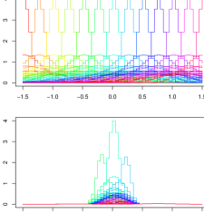
Figure 2: The initial quantization set $\mathcal{Q}^{0}_{n}$ (top graph) and the approximation of the optimal quantization set in the stochastic gradient descent methods in 500 steps (bottom graph)

Source: own calculations

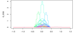
Figure 3: The selection of the essential elements of the quantization set $\mathcal{Q}^{500}_{n}$ (25 out of 65 elements)

Source: own calculations

The procedure requires to construct the incremental function $H$ which defines the corrections of $\mathcal{Q}^{0}_{n}$ leading in the limit to the optimal quantization set. The incremental function is derived by the formal differentiation under $\bar{\mathbf{E}}$ of the distortion function $D_{n}(Q)$ for a given realization $\hat{r}$ of return $R^{l}$. Namely, in the special case of 1-dimensional process $Y$ any quantization set $\mathcal{Q}$ can be represented by the matrix from $\mathcal{M}^{n\times m_{n}}$ where $(k,m)$ element is defined as the value of the $k$th element of the set $\mathcal{Q}$ evaluated at the $m$th argument from $Z_{n}$. Then, the function $H\colon\mathcal{M}^{n\times m_{n}}\times\mathbb{R}\to\mathcal{M}^{n\times m_{n}}$ is defined as

$$H_{k,m}(\mathcal{Q},\hat{r})\colon={\partial\over\partial\hat{r}}\varrho(z_{k},\hat{r})\left(\varrho(z_{k},\hat{r})-g_{m}(k)\right).$$

Since in the example the densities $\phi$ and $\psi$ in the example are smooth then the derivative of $\varrho$ is well-defined. Then for a given sequence $\{\beta_{i}\}_{i\in\mathbb{N}}$ satisfying the usual regularity conditions ($\sum\beta_{i}=\infty$ and $\sum\beta^{2}_{i}<\infty$) the following sequence of the quantization sets converge to the optimal one (see Shapiro and Wardi [22] for convergence results):

$$\mathcal{Q}_{n}^{m+1}=\max\left\{\mathcal{Q}_{n}^{m}+\beta_{m+1}H(\mathcal{Q}_{n}^{m},R^{l}(\omega_{m+1})),0\right\}.$$

Applying this recursive procedure for $\mathcal{Q}_{n}^{m}$ with 500 iterations of $m$ we obtain the modified set $\mathcal{Q}^{500}_{n}$ which is graphically presented on figure 2, bottom panel. Firstly, one crucial advantage of $\mathcal{Q}_{n}^{500}$ is the reduction of the domain of the densities from the initial $[-1.5,1.5]$ to $[-0.5,0.5]$ where they are essentially different from 0. This decreases the dimensionality of the numerical problem since the same number of points $Z_{n}$ can be denser allocated on the smaller interval $[-0.5,0.5]$. Secondly, we can drop the densities from $\mathcal{Q}_{n}^{500}$ which are very similar to each other and we take into account only a subset $\mathcal{Q}_{n}^{ess}\subset\mathcal{Q}_{n}^{500}$ if the densities. Namely, we apply the following procedure:

1. $\mathcal{Q}_{n}^{ess}\colon=\mathcal{Q}_{n}^{500}$; eps=0.1;

2. REPEAT i

3. Chose a pair of densities $q_{1}\in\bar{Q}^{ess}$ and $q_{2}\in\bar{Q}^{ess}$;

4. IF $\frac{\sum_{z\in Z_{n}}|q_{1}(z)-q_{2}(z)|}{\sum_{z\in Z_{n}}|q_{1}(z)|}<$eps THEN $\mathcal{Q}_{n}^{ess}\colon=\mathcal{Q}_{n}^{ess}/\{q_{2}\}$;

5. i:=i+1;

6. UNTIL i==5000;

the application of which gives the quantization set consisting of 25 unnormalized densities.

It should be underlined that functions $\varrho$ representing the beliefs about $Y$, described by recursion 7, are not necessarily densities. They are unnormalized densities. An example of the evolution of beliefs is presented on the figure 4.

Figure 4: Evolution of beliefs with prior at time $T-9$ equal to the normal distribution with mean $0.1$ and standard deviation $0.2$

Note: Each box shows a density which is recursively obtained using equation 7, i.e. the density on the box $T-n$ is obtained from the formula 7 with $\varrho_{T-n-1}$ equal to the density from the box $T-n-1$ and $\varrho_{T-9}\equiv\phi_{0.1,0.2}$.
Source: own calculations

The number of nodes of the portfolio values, which is 41, multiplied by the number of the densities in the density quantization set equal to 25 gives 1025 arguments of $\widehat{V}(t,\cdot,\cdot)$.

Searching for the optimal consumption and investment for a given point of time $t$, the current wealth $\bar{x}$ and the beliefs about the unobserved factors driving the volatility on the market, we discretize the space of investors decisions. We were looking for the maximum expected value of the value function $\widehat{V}(t+1,x^{c,\pi}(t+1),\varrho_{t+1})$ among $c\in\{0.00\bar{x},0.05\bar{x},0.10\bar{x},\dots,0.95\bar{x},1.00\bar{x}\}$ and $\pi\in\{0.00\bar{x},0.05\bar{x},0.10\bar{x},\dots,0.95\bar{x},1.00\bar{x}\}$.

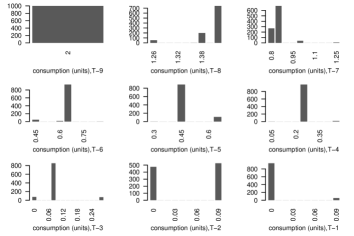
Figure 5: Distribution of the optimal consumption for different points of time

Note: histograms for 1000 simulation of the risky asset dynamics. $T-n$ means $n$ time periods before the time horizon $T$.
Source: own calculation

The four main components of the solution of the numerical optimization were presented: the consumption, the investment in the risky asset and the risk-free asset and the value of the optimal portfolio. Assuming that the investor possesses 6 units of the initial capital we generated his wealth paths along the estimated consumption and investment policies. We perform 1000 simulations of the risky asset prices and we construct the corresponding consumption and investment paths according to the approximate optimal policy.

The results of the simulation suggest that the optimally behaving investor consume about half of the initial wealth during the first two periods and then gradually decreases the consumption rate (see figure 5). In the period $t=6$ the investor is left with less then 1 units of wealth. In the last three periods he consumes only about 0.1 units of his portfolio, almost irrespective of the market situation (i.e. independent of the evolution of the risky asset prices).

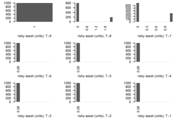
Figure 6: Distribution of the optimal investment into the risky asset for different points of time

Note: histograms for 1000 simulation of the risky asset dynamics. $T-n$ means $n$ time periods before the time horizon $T$.
Source: own calculation

Conversely, his investment decisions are much more dependent on the market trends and on the time of decision making. His stronger beliefs about unfavorable volatility (about $y$) decrease his propensity to invest into the risky asset. The investor allocates quite a small part of his wealth in the risky project $S_{1}$ only in the first two periods (see figure 6). The closer to the terminal time $T$ the more he is inclined to allocate his current wealth into the risk-free asset $S_{0}$ (see figure 7). As the figure 8 indicates, the terminal wealth reaches almost 0 units.

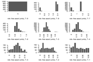
Figure 7: Distribution of the optimal investment into the risk-free asset for different points of time

Note: histograms for 1000 simulation of the risky asset dynamics. $T-n$ means $n$ time periods before the time horizon $T$.
Source: own calculation

Figure 8: Distribution of the optimal value of portfolio for different points of time

Note: histograms for 1000 simulation of the risky asset dynamics. $T-n$ means $n$ time periods before the time horizon $T$.
Source: own calculation

Even though the set of beliefs seems to be only roughly approximated by 30 density functions, the simulation reflects the behavior of a rational investor in a quite reasonable and intuitive way. However, the computational burden of the numerical procedure makes it difficult to support investment decisions on a market for multiple assets unless the complexity of the stochastic volatility part of the model is substantially reduced. In fact the minimal error of the estimate of the value function $V$ that can be attained in the numerical example and given by the constant $C_{n.M_{0}}$ multiplied by the factor $\delta\frac{1-\delta^{T}}{1-\delta}$ (see theorem 3.2) is equal to 0.81 which is about 12% of the utility of the initial wealth.

However, the proposed quantization framework follows the promising avenue of research on the portfolio optimization under the partial observation of the stochastic volatility. It shows that the nonlinear filtering can be tractable even in the dynamic programming setting. From the financial point of view, the incomplete information is a very important driver of the market dynamics and its influence on the economic agents’ optimal choice is worse studying. Certainly, a more efficient numerical implementation of the algorithm is required.

5 Conclusions

We solved the dynamic optimal consumption/investment strategy under partial observation of economic factors determining asset price movements by means of the numerical method. The special variation of the quantization technique reduced the originally infinite dimensional problem to the finite state space exercise. We successfully developed the algorithm to solve the consumption / investment problem on the stylized market for 2 tradable assets and 1 unhedgable economic factor.

The extension of the paper can be devoted to a study of the stability of the algorithm solving numerically the optimal portfolio choice with consumption. The first important question remains how the results of the simulation change between two different sets of randomly generated asset returns. The second one could be related to the size of quantization set that would in practice give an assumed accuracy of numerical optimal strategies.

We transformed the partial observation to the full observation problem, assuming that the shocks affecting prices and economic factors are independents. However, existing methods of stochastic volatility estimation [11] do not need shocks to be orthogonal. It would be interesting to develop a model of consumption/investment with imperfect observation and correlation of volatility and idiosyncratic shocks in the asset price movements.

Appendix A Filters

The following lemma is the most crucial in obtaining filters of partially observed processes. It states that $Y$s and $R_{i}^{l}$s are independent in $(\mathcal{F}^{lR},\bar{\mathbf{P}})$. After disentangling $Y$ from $R^{l}$, the evolution of the variable $Y$ can be reformulated to a recursive equation of measures on $(\Omega,\mathbb{F}^{lR})$.

Lemma A.1

The processes $Y$ and $R^{l}$ are independent in $\mathcal{F}^{lR}$ under $\bar{\mathbf{P}}$.

Proof: Let us take two Borel functions $f_{1}$ and $f_{2}$. Then

$$\bar{\mathbf{E}}\left.\left[f_{1}(Y(t))f_{2}(R^{l}(t))\right|\mathcal{F}^{lR}_{t-1}\right] = {\mathbf{E}\left.\left[\Lambda_{t}^{-1}f_{1}(Y(t))f_{2}(R^{l}(t))\right|\mathcal{F}^{lR}_{t-1}\right]\over\mathbf{E}\left.\left[\Lambda_{t}^{-1}\right|\mathcal{F}^{lR}_{t-1}\right]}$$ (18)

$$= {\mathbf{E}\left.\left[\lambda_{t}^{-1}f_{1}(Y(t))f_{2}(R^{l}(t))\right|\mathcal{F}^{lR}_{t-1}\right]\over\mathbf{E}\left.\left[\lambda_{t}^{-1}\right|\mathcal{F}^{lR}_{t-1}\right]}$$

since $\Lambda^{-1}_{t}=\lambda^{-1}_{t}\Lambda^{-1}_{t-1}$ and $\Lambda^{-1}_{t-1}$ is $\mathcal{F}^{Y}_{t-1}$-measurable. For brevity $\tilde{y}\colon\!\!=Y(t-1)$. Let us take the denominator in 18 and

$$\mathbf{E}\left.\left[\lambda_{t}^{-1}\right|\mathcal{F}^{lR}_{t-1}\right]=$$

$$=\mathbf{E}\left.\left[{\det(\sigma(Y(t)))\phi(R^{(l)}(t))\over\phi\Big{(}\sigma^{-1}(Y(t))[R^{(l)}(t)-\mu(Y(t))]\Big{)}}{\det(\sigma_{Y})\psi(Y(t))\over\psi\Big{(}\sigma_{Y}^{-1}[Y(t)-\tilde{y}-\alpha(\bar{y}-\tilde{y})]\Big{)}}\right|\mathcal{F}^{lR}_{t-1}\right]$$

$$=\mathbf{E}\left.\left[{\phi\big{(}\mu(Y(t))+\sigma(Y(t))\epsilon(t)\big{)}\over\det(\sigma^{-1}(Y(t)))\phi\left(\epsilon(t)\right)}{\psi\big{(}\tilde{y}-\alpha(\bar{y}-\tilde{y})+\sigma_{Y}\xi(t)\big{)}\over\det(\sigma^{-1}_{Y})\psi(\xi(t))}\right|\mathcal{F}^{lR}_{t-1}\right].$$

Put

$$p_{1}\colon\!\!={\psi\big{(}\tilde{y}-\alpha(\bar{y}-\tilde{y})+\sigma_{Y}\xi(t)\big{)}\over\det(\sigma^{-1}_{Y})\psi(\xi(t))}.$$

Then

$$\mathbf{E}\left.\left[\lambda_{t}^{-1}\right|\mathcal{F}^{lR}_{t-1}\right]=\mathbf{E}\left.\left[p_{1}\mathbf{E}\left[{{\phi\big{(}\mu(Y(t))+\sigma(Y(t))\epsilon(t)\big{)}\over\det(\sigma^{-1}(Y(t)))\phi\left(\epsilon(t)\right)}}\Big{|}\sigma(\mathcal{F}^{lR}_{t-1},\mathcal{F}^{Y}_{t})\right]\right|\mathcal{F}^{lR}_{t-1}\right].$$

The variable $\epsilon(t)$ is independent of $\mathcal{F}_{t-1}^{lR}$ so we can integrate with respect to the density $\phi$

$$\mathbf{E}\left.\left[\lambda_{t}^{-1}\right|\mathcal{F}^{lR}_{t-1}\right]=\mathbf{E}\left.\left[p_{1}\int_{\mathbb{R}^{N}}{\phi\big{(}\mu(Y(t))+\sigma(Y(t))\hat{\epsilon}\big{)}\over\det(\sigma^{-1}(Y(t)))\phi\left(\hat{\epsilon}\right)}\phi(\hat{\epsilon})\mathrm{d}\hat{\epsilon}\right|\mathcal{F}^{lR}_{t-1}\right].$$

By changing variables with the diffeomorphism $\Theta(\hat{\epsilon})=\sigma^{-1}(Y(t))\hat{\epsilon}$, with a given fixed $\omega$, as follows $\int_{\Theta(\mathbb{R}^{N})}G(\hat{\epsilon})\mathrm{d}\hat{\epsilon}=\int_{\mathbb{R}^{N}}(\Theta\circ G)(\hat{\epsilon})\det(\Theta^{\prime}(\hat{\epsilon}))\mathrm{d}\hat{\epsilon}$ we get

$$\mathbf{E}\left.\left[\lambda_{t}^{-1}\right|\mathcal{F}^{lR}_{t-1}\right]=\mathbf{E}\left.\left[p_{1}\int_{\mathbb{R}^{N}}\phi\big{(}\mu(Y(t))+\hat{\epsilon}\big{)}\mathrm{d}\hat{\epsilon}\right|\mathcal{F}^{lR}_{t-1}\right]$$

$$=\mathbf{E}\left.\left[\mathbf{E}\left[{\psi\big{(}\tilde{y}-\alpha(\bar{y}-\tilde{y})+\sigma_{Y}\xi(t)\big{)}\over\det(\sigma^{-1}_{Y})\psi(\xi(t))}\Big{|}\sigma(\mathcal{F}^{lR}_{t-1},\mathcal{F}^{Y}_{t-1})\right]\right|\mathcal{F}^{lR}_{t-1}\right]$$

$$=\mathbf{E}\left.\left[\int_{\mathbb{R}^{K}}{\psi\big{(}\tilde{y}-\alpha(\bar{y}-\tilde{y})+\sigma_{Y}\hat{\xi}\big{)}\over\det(\sigma^{-1}_{Y})\psi(\hat{\xi})}\psi(\hat{\xi})\mathrm{d}\hat{\xi}\right|\mathcal{F}^{lR}_{t-1}\right]\equiv 1,$$

observing that $\xi(t)$ is independent of $\mathcal{F}^{lR}_{t-1}$.

Let us take

$$\mathbf{E}\left.\left[\lambda_{t}^{-1}f_{1}(Y(t))f_{2}(R^{l}(t))\right|\mathcal{F}^{lR}_{t-1}\right]=$$

$$=\mathbf{E}\left.\left[p_{1}f_{1}(Y(t))f_{2}(R^{l}(t)){\phi\big{(}\mu(Y(t)))+\sigma(Y(t))\epsilon(t)\big{)}\over\det(\sigma^{-1}(Y(t)))\phi\left(\epsilon(t)\right)}\right|\mathcal{F}^{lR}_{t-1}\right]$$

$$=\mathbf{E}\left.\left[p_{1}f_{1}(Y(t))\mathbf{E}\left[f_{2}(R^{l}(t)){\phi\big{(}\mu(Y(t))+\sigma(Y(t))\epsilon(t)\big{)}\over\det(\sigma^{-1}(Y(t)))\phi\left(\epsilon(t)\right)}\Big{|}\sigma(\mathcal{F}^{lR}_{t-1},\mathcal{F}_{t}^{Y})\right]\right|\mathcal{F}^{lR}_{t-1}\right].$$

A similar argument about independence of $\epsilon(t)$ and $\mathcal{F}^{lR}_{t-1}$ gives

$$\mathbf{E}\left.\left[\lambda_{t}^{-1}f_{1}(Y(t))f_{2}(R^{l}(t))\right|\mathcal{F}^{lR}_{t-1}\right]=$$

$$=\mathbf{E}\left.\left[f_{1}(Y(t))p_{1}\int_{\mathbb{R}^{N}}f_{2}(\mu(Y(t))+\sigma(Y(t))\hat{\epsilon}){\phi\big{(}\mu(Y(t))+\sigma(Y(t))\hat{\epsilon}\big{)}\over\det(\sigma^{-1}(Y(t)))}\mathrm{d}\hat{\epsilon}\right|\mathcal{F}^{lR}_{t-1}\right]$$

and after the diffeomorphic change of variables

$$=\mathbf{E}\left.\left[f_{1}(Y(t))p_{1}\mathbf{E}\left[f_{2}(R^{l}(t))\big{|}\mathcal{F}^{lR}_{t-1}\right]\right|\mathcal{F}^{lR}_{t-1}\right]$$

$$=\mathbf{E}\left.\left[f_{1}(Y(t)){\psi\big{(}\tilde{y}-\alpha(\bar{y}-\tilde{y})+\sigma_{Y}\xi(t)\big{)}\over\det(\sigma^{-1}_{Y})\psi(\xi(t))}\mathbf{E}\left[f_{2}(R^{l}(t))\big{|}\mathcal{F}^{lR}_{t-1}\right]\right|\mathcal{F}^{lR}_{t-1}\right]$$

$$=\mathbf{E}\left.\left[\int_{\mathbb{R}^{K}}f_{1}(\tilde{y}-\alpha(\bar{y}-\tilde{y})+\sigma_{Y}\hat{\xi}){\psi\big{(}\tilde{y}-\alpha(\bar{y}-\tilde{y})+\sigma_{Y}\hat{\xi}\big{)}\over\det(\sigma^{-1}_{Y})}\mathrm{d}\hat{\xi}\cdot\mathbf{E}\left[f_{2}(R^{l}(t))\big{|}\mathcal{F}^{lR}_{t-1}\right]\right|\mathcal{F}^{lR}_{t-1}\right]$$

$$=\mathbf{E}\left.\left[\mathbf{E}\left[f_{1}(Y(t))\big{|}\mathcal{F}^{lR}_{t-1}\right]\cdot\mathbf{E}\left[f_{2}(R^{l}(t))\big{|}\mathcal{F}^{lR}_{t-1}\right]\right|\mathcal{F}^{lR}_{t-1}\right]$$

$$=\mathbf{E}\left[f_{1}(Y(t))\big{|}\mathcal{F}^{lR}_{t-1}\right]\cdot\mathbf{E}\left[f_{2}(R^{l}(t))\big{|}\mathcal{F}^{lR}_{t-1}\right].$$

Taking $f_{1}(z)=\mathbf{1}_{A}(z)$ and $f_{2}(z)=\mathbf{1}_{B}(z)$ for $A,B\in\mathcal{F}^{lR}_{t}$ we obtained

$$\mathbf{P}\left(\{R^{l}(t)\in A\}\cap\left\{Y(t)\in B\right\}\big{|}\mathcal{F}^{lR}_{t-1}\right)=\mathbf{E}\left.\left[f_{1}(R^{l}(t))f_{2}(Y(t))\right|\mathcal{F}^{lR}_{t}\right]=$$

$$=\mathbf{E}\left.\left[f_{1}(R^{l}(t))\right|\mathcal{F}^{lR}_{t}\right]\mathbf{E}\left.\left[f_{2}(Y(t))\right|\mathcal{F}^{lR}_{t}\right]=\mathbf{P}\left(R^{l}(t)\in A\big{|}\mathcal{F}^{lR}_{t-1}\right)\mathbf{P}\left(Y(t)\in B\big{|}\mathcal{F}^{lR}_{t-1}\right).$$

$\Box$

Proof: [Theorem 2.1] For an arbitrary Borel function $f$ let us take

$$\int_{\mathbb{R}^{K}}f(z)\varrho_{t}(z)\mathrm{d}z=\bar{\mathbf{E}}\left.\left[\Lambda_{t}f(Y(t))\right|\mathcal{F}^{lR}_{t}\right]=$$

$$=\bar{\mathbf{E}}\left.\left[\Lambda_{t-1}{\phi\Big{(}\sigma^{-1}(Y(t))[R^{(l)}(t)-\mu(Y(t))]\Big{)}\over\det(\sigma(Y(t)))\phi(R^{(l)}(t))}{\psi\Big{(}\sigma_{Y}^{-1}[Y(t)-\tilde{y}-\alpha(\bar{y}-\tilde{y})]\Big{)}\over\det(\sigma_{Y})\psi(Y(t))}f(Y(t))\right|\mathcal{F}^{lR}_{t}\right]$$

$$=\bar{\mathbf{E}}\left[\Lambda_{t-1}\mathbf{E}\left[{\phi\Big{(}\sigma^{-1}(Y(t))[R^{(l)}(t)-\mu(Y(t))]\Big{)}\over\det(\sigma(Y(t)))\phi(R^{(l)}(t))}\right.\right.$$

$$\qquad\qquad\qquad\qquad\left.\left.{\psi\Big{(}\sigma_{Y}^{-1}[Y(t)-\tilde{y}-\alpha(\bar{y}-\tilde{y})]\Big{)}\over\det(\sigma_{Y})\psi(Y(t))}f(Y(t))\Bigg{|}\sigma(\mathcal{F}^{lR}_{t},\mathcal{F}^{Y}_{t-1})\right]\Bigg{|}\mathcal{F}_{t}^{lR}\right]$$

$$=\bar{\mathbf{E}}\left.\left[\Lambda_{t-1}\int_{\mathbb{R}^{K}}{\phi\Big{(}\sigma^{-1}(z)[R^{(l)}(t)-\mu(z)]\Big{)}\over\det(\sigma(z))\phi(R^{(l)}(t))}{\psi\Big{(}\sigma_{Y}^{-1}[z-\tilde{y}-\alpha(\bar{y}-\tilde{y})]\Big{)}\over\det(\sigma_{Y})\psi(z)}f(z)\psi(z)\mathrm{d}y\right|\mathcal{F}^{lR}_{t}\right].$$

The inner process is the function of $Y(t-1)$ and $\Lambda_{t-1}$ so we can integrate with respect to $\varrho_{t-1}(z)$ in the following

$$\int_{\mathbb{R}^{K}}f(z)\varrho_{t}(z)\mathrm{d}z = \int_{\mathbb{R}^{K}}\left(\int_{\mathbb{R}^{K}}{\Phi(z,R^{l}(t))\over\phi(R^{l}(t))}\Psi(z,y)f(z)\mathrm{d}z\right)\varrho_{t-1}(y)\mathrm{d}y$$

$$= \int_{\mathbb{R}^{K}}f(z){\Phi(z,R^{l}(t))\over\phi(R^{l}(t))}\left(\int_{\mathbb{R}^{K}}\Psi(z,y)\varrho_{t-1}(y)\mathrm{d}y\right)\mathrm{d}z.$$

Since $f$ is the arbitrary function the identity 7 holds.
$\Box$

Appendix B The constant $v_{N}$ in the error estimate in lemma 3.3

Changing the limits of integration in the integral

$$\int_{[M_{0},+\infty)^{N}}|x|^{-p}\mathrm{d}x$$

to the polar ones with

$$F(w,\alpha_{1},\dots,\alpha_{N})=\left[\begin{matrix}\hfill w\cos\alpha_{1}\cos\alpha_{2}\cos\alpha_{3}\dots\cos\alpha_{N-1}\cr\hfill w\sin\alpha_{1}\cos\alpha_{2}\cos\alpha_{3}\dots\cos\alpha_{N-1}\cr\hfill w\sin\alpha_{2}\cos\alpha_{3}\dots\cos\alpha_{N-1}\cr\vdots\cr\hfill w\sin\alpha_{N-2}\cos\alpha_{N-1}\cr\hfill w\sin\alpha_{N-1}\end{matrix}\right]$$

we obtain

$$\int_{[M_{0},+\infty)^{N}}|x|^{-p}\mathrm{d}x=\int_{[M_{0},+\infty)\times[0,2\pi]\times[-{\pi\over 2}{\pi\over 2}]^{N-2}}r^{-p}|\det F^{\prime}|\mathrm{d}w\mathrm{d}\alpha_{1}\alpha_{2}\dots\alpha_{N-1}=$$

$$\int_{[M_{0},+\infty)}w^{-p}w^{N-1}\int_{[0,2\pi]}1\mathrm{d}\alpha_{1}\int_{[-{\pi\over 2}{\pi\over 2}]}\cos\alpha_{2}\mathrm{d}\alpha_{2}\dots\int_{[-{\pi\over 2}{\pi\over 2}]}(\cos\alpha_{N-1})^{N-2}\mathrm{d}\alpha_{N-1}.$$

Let us denote $I_{n}\colon=\int_{-{\pi\over 2}}^{\pi\over 2}\cos^{n}t\mathrm{d}t.$ Note that $I_{0}=\pi$ and $I_{1}=2$. Integrating by parts

$$\int_{-{\pi\over 2}}^{\pi\over 2}\cos t\cos^{n-1}t\mathrm{d}t = \sin t\cos^{n-1}t\Big{|}_{-{\pi\over 2}}^{\pi\over 2}+\int_{-{\pi\over 2}}^{-{\pi\over 2}}\sin^{2}t\cos^{n-2}t\mathrm{d}t$$

$$I_{n} = 0+nI_{n-1}-nI_{n},$$ (19)

thus

$$n=2k \Rightarrow I_{n}={n!!\over(n+1)!!}\pi,$$

$$n=2k+1 \Rightarrow I_{n}=2{n!!\over(n+1)!!}.$$

Then

$$v_{N} = {2\pi\over N-p}\prod_{j=2}^{N-1}\int_{[-{\pi\over 2},{\pi\over 2}]}(\cos t)^{j-1}\mathrm{d}t$$ (20)

$$= {2\pi\over N-p}\prod_{j=1}^{N-2}2^{j\mathrm{mod}2}\pi^{(j+1)\mathrm{mod}2}{j!!\over(j+1)!!}$$

$$= \left\{\begin{matrix}{2\pi\over(N-p)(N-2)!!}(2\pi)^{{N-2\over 2}},\hfill&\mathrm{if}\ N=2k\hfill\cr{2\pi\over(N-p)(N-2)!!}2^{{N-3\over 2}}\pi^{{N-3\over 2}+1},\hfill&\mathrm{if}\ N=2k+1\hfill\cr\end{matrix}\right.$$

References

- Baghery and Øksendal [2007] F. Baghery, B. Øksendal A maximum principle for stochastic control with partial information. Stochastic Analysis and Applications 25 (2007) 705–717.
- Barndorff-Nielsen et al. [2002] O.E. Barndorff-Nielsen, E. Nicolato, N. Shephard, Some recent developments in stochastic volatility modelling, Quantitative Finance 2(1) (2002) 11–23.
- Beneš et al. [2004] V. Beneš, I. Karatzas, D. Ocone, H. Wang, Control with Partial Observations and an Explicit Solution of Mortensen’s Equation, Applied Mathematical Optimisation, 49 (2002) 217–239.
- Bensoussan [1992] A. Bensoussan, Stochastic Control of Partially Observable Systems, Cambridge University Press, Cambridge, 1992.
- Bertsekas [1976] D. Bertsekas, Dynamic Programming and Stochastic Control, New York: Academic Press, 1976.
-
Brendle [2005]
S. Brendle, Portfolio Selection under Partial Observation and Filtering,
preliminary version of working paper, Prinston University (2005)
http://papers.ssrn.com/sol3/papers.cfm?abstract_id=590362. - Carmona and Ludkovsky [2004] R. Carmona, M. Ludkovski, Convenience yield model with partial observations and exponential utility, Princeton working paper (2004).
- Corsi et al. [2008] M. Corsi, H. Pham, W. Runggaldier, Numerical approximation by quantization of control problems in finance under partial observations, Mathematical modeling and numerical methods in finance, in A. Bensoussan, Q. Zhang (Eds.), Handbook of Numerical analysis (special volume), 2008.
- Del Moral et al. [2001] P. Del Moral, J. Jacod, Ph. Protter, The Monte-Carlo methods for filtering with discrete time observations, Probability Theory and Related Fields 120 (2001) 346–368.
- Desai et al. [2003] R. Desai, T. Lele., F. Viens, A Monte-Carlo method for portfolio optimization under partially observed stochastic volatility, IEEE International Conference on Computational Intelligence for Financial Engineering, Proceedings 2003.
- Durham [2007] G. Durham, Monte Carlo methods for estimating, smoothing and filtering one- and two-factor stochastic volatility models, Journal of Econometrics 133 (2007) 273–305.
- Elliot and Miao [2006] R. Elliot, H. Miao, Stochastic Volatility Model with Filtering, Stochastic Analysis and Applications 24 (2006) 661–683.
- Hałaj [2008] G. Hałaj, Risk-based decisions on the asset structure of a bank under economic information, Applied Mathematical Finance 15(4) (2008) 305–329.
- Krishnamurthy and Le Gland [1996] V. Krishnamurthy, F. Le Gland, the Discretization of Continuous-Time Filters and Smoothers for HMM Parameter Estimation, IEEE Transactions on Information Theory 42(3) (1996) 593–605.
- Lakner [1995] P. Lakner, Utility maximization with partial information, Stochastic Processes and their Application 56 (1995) 247–273.
- Pagès et al. [2004a] G. Pagès, H. Pham, J. Printemps, An Optimal Markovian Quantization Algorithm for Multidimensional Stochastic Control Problems, Stochastics and Dynamics 4(4) (2004) 501–545.
- Pagès et al. [2004b] G. Pagès, H. Pham, J. Printemps, Optimal quantization methods and applications to numerical problems in finance, in: S. Rachev (Ed.), Handbook on Numerical Methods in Finance, Birkhauser, Boston, 2004, pp. 253–298.
- Pagès and Pham [2005] G. Pagès, H. Pham, Optimal quantization methods for nonlinear filtering with discrete-time observations, Bernoulli 11(5) (2005) 893-–932.
- Pham and Quenez [2001] H. Pham, M.-C. Quenez, Optimal Portfolio in Partially Observed Stochastic Volatility Models, The Annals of Applied Probability 11(1) (2001) 210–238.
- Runggaldier and Stettner [1994] W. Runggaldier, Ł. Stettner, Approximation of Discrete Time Partially Observed Control Problems, Applied Mathematics Monographs CNR, Pisa, 1994.
- Sass and Haussmann [2004] J. Sass, U.G. Haussmann, Optimizing the terminal wealth under partial information: The drift process as a continuous time Markov chain, Finance and Stochastics 8 (2004) 553–577.
- Shapiro and Wardi [1996] A. Shapiro, Y. Wardi, Convergence Analysis of Gradient Descent Stochastic Algorithms, Journal of optimization theory and applications 91(2) (1996) 439–454.
- Sørensen [2000] H. Sørensen, Simulated Likelihood Approximations for Stochastic Volatility Models, Scandinavian Journal of Statistics 30(2) (2003) 257–276.
- Stettner [2004] Ł. Stettner, Risk-Sensitive Portfolio Optimization With Completely and Partially Observed Factors, IEEE Transactions on Automatic Control 49(3) (2004) 457–464.