Will the US Economy Recover in 2010?
A Minimal Spanning Tree Study

Abstract

We calculated the cross correlations between the half-hourly times series of the ten Dow Jones US economic sectors over the period February 2000 to August 2008, the two-year intervals 2002–2003, 2004–2005, 2008–2009, and also over 11 segments within the present financial crisis, to construct minimal spanning trees (MSTs) of the US economy at the sector level. In all MSTs, a core-fringe structure is found, with consumer goods, consumer services, and the industrials consistently making up the core, and basic materials, oil & gas, healthcare, telecommunications, and utilities residing predominantly on the fringe. More importantly, we find that the MSTs can be classified into two distinct, statistically robust, topologies: (i) star-like, with the industrials at the center, associated with low-volatility economic growth; and (ii) chain-like, associated with high-volatility economic crisis. Finally, we present statistical evidence, based on the emergence of a star-like MST in Sep 2009, and the MST staying robustly star-like throughout the Greek Debt Crisis, that the US economy is on track to a recovery.

1 Introduction

In the CBS ‘60 Minutes’ interview televised on 15 March 2009, Ben Bernanke predicted that the recession triggered by the global financial crisis will end in 2009, and the US economy will recover in 2010 [1]. While we will never know whether Bernanke made the prediction based on his gut feelings, or on simulation results from some sophisticated macroeconomic model, what we do know is that the prediction sparked intense public debate on whether the Chairman of the US Federal Reserve was overly optimistic. Given that the financial industry was still reeling from the massive October 2008 slide, reactions to Bernanke’s statement must be especially strong. We also know that the US Federal Reserve does not appear to be behind its Chairman: up till September 2010, the interest rate has not been raised [2], even though there has been calls from within the Federal Reserve system to tighten the money supply [3]. This has led to mounting concerns from economists that the oversupply of government money, in the form of an interest rate that is nearly zero, will cause an inflation when the economy recovers [4, 5]. In fact, a commentator argued that US stimulus money is fueling property bubbles all over Asia, and warned that the global economy will crash once again in 2012 when the Feds rein in their easy money [6].

In January 2004, there was a similar call by economists to raise interest rates [7], when the US economy was showing signs of coming out of the technology bubble crisis. The Federal Reserve responded hesitantly only in June 2004 [2]. We can understand the concern of the US government then, and possibly also now: how do we know that the early signs will lead on to a recovery that will strengthen and stay the course? From these historical and contemporary lessons, we know that a more sensitive and more robust indicator of economic recovery is needed. While much work has been done on developing and validating reliable precursor signatures (also called leading indicators) for the onset of financial crises (see for example, Refs. [8, 9, 10, 11, 12, 13, 14]), and understanding such economic disasters in general (see for example, Refs. [15, 16, 17, 18, 19, 20]), less has been done to find robust indicators of economic recovery (see for example, Refs. [21, 22, 23]). In this work, we hope to address this important gap.

Recently, we adapted the recursive entropic segmentation method [24, 25] developed by Bernaola-Galván and coworkers for biological sequence segmentation, and applied it to financial time series segmentation [26]. Based on our segmentation of the Dow Jones Industrial Average (DJIA) time series between 1997 and 2008, we saw that the US economy, as measured by the DJIA, switched between a high-volatility crisis phase and a low-volatility growth phase. The first crisis phase lasted from mid-1998 to mid-2003, coinciding with the US technology bubble and the ensuing economic recession. The second crisis phase started in mid-2007, coinciding with the US Subprime Crisis and the ensuing global financial crisis. More interestingly, we could also identify a year-long series of precursor shocks prior to the mid-1998 and mid-2007 onsets of two crisis phases, as well as a year-long series of inverted shocks prior to the mid-2003 economic recovery. The series of inverted shocks started with the mid-2002 Dow Jones low, so if we believe the internal dynamics of the US economy had not changed from the previous financial crisis to the present financial crisis, we would naively expect the US economy to recover one year after the March 2009 lows, i.e. the second quarter of 2010, give and take.

Clearly, a single study of a single time series spanning only two financial crises and one growth period is hardly enough statistical evidence in Bernanke’s favor. To enhance the statistical significance of features seen in the segmented DJIA time series, we carried out a cross-section study, comparing the segmented time series of the ten Dow Jones US (DJUS) economic sector indices [27]. By identifying the sequences of onsets in the ten DJUS indices, we find sectors in the US economy going first to last into the present financial crisis in merely two months! While we may or may not have an extended sequence of precursor shocks to work with for predicting market crashes and financial crisis (see the recent update [28] on the heroic efforts by Sornette and coworkers), when the dominoes are set in motion policy makers will have a month or two to contain the crisis. Since this financial crisis eventually spread globally, we will have to wait for the next potential crisis to find out if containment is at all possible. We do know, however, that the US Federal Reserve acted promptly, announcing the first of a series of interest rate cuts in August 2007. Unfortunately, as detailed in Ref. [27], we saw these rate cuts rapidly losing effectiveness. A critical discussion on the actions taken by the US Federal Reserve can be found in Ref. [29].

In the same comparative study, we also identified the sequence of economic recoveries in the different US economic sectors. The excruciatingly slow complete economic recovery from the previous financial crisis, defined as consistent growth in the first sector to consistent growth in the last sector, took one and a half years. Given this long time scale, developing robust indicators to detect economic recovery, and thereafter designing timely stimulus packages, should be easier than finding sensitive indicators that would warn us of an impending financial crisis. We would imagine that tracking slow month-to-month indicators should be enough to give us a confident forecast on the start of growth, but all through the second half of 2009 and 2010 to date, we hear commentators mostly urging caution [30, 31, 32, 33, 34, 35, 36, 37]. We believe this cautious outlook can be blamed partly on swings in the stock markets, which always become strong when things are taking a turn for the better or for the worst. Perhaps the way to allay such market-driven fears is to extract convincing signs from the high-frequency stock-market data itself. Based on these signs, policy makers can then tell more confidently that the economy will recover in a matter of months, and start planning measures to further stimulate the recovery.

In this paper, which is organized into six sections, we report a minimal spanning tree (MST) study of the segmented time series of the ten DJUS economic sector indices. In Section 2, we describe the data sets studied, and the statistical methods used to analyze them. In Section 3, we examine the gross structure of the 10-sector MST over the 2000 to 2009 period, as well as those over the 2002–2003 crisis period, the 2004–2005 growth period, and the 2008–2009 crisis period. We explain the macroeconomic significance of the core-fringe structure of the MSTs, and also suggest why the MSTs organize themselves into a star topology during growth, and into a chain topology during crisis. Then, in Section 4, we construct MSTs within segments associated with distinct macroeconomic phases to study the correlational dynamics within the US economy. We again find that the MST is star-like in low-volatility segments, and chain-like in high-volatility segments. This tells us that the star-like MST is a robust and reliable character of economic well being. By combining temporal information obtained through statistical segmentation and clustering, we show that volatility shocks always start at the fringe and propogate inwards. Some of the links to leader sectors have anomalously high cross-correlations. We also check whether such volatility shocks have a more domestic or more global origin. Finally in Section 5, by examining a nearly contiguous sequence of corresponding segments, we look at how the MST rearranges in the pre-recovery periods for both the previous and the current financial crises. We found very violent rearrangements prior to the previous economic recovery. For the present financial crisis, we can see clear signatures of star-to-chain and chain-to-star rearrangements, accompanied by the expected changes in market volatilities and cross-correlations. This suggests that the US market has become more efficient, as far as processing information is concerned, over the past 5–10 years. After predicting that the US economy will recover in early 2010, we summarize our findings in Section 6.

2 Data and methods

2.1 Data

Tic-by-tic data for the ten Dow Jones US (DJUS) economic sector indices (see Table 1 for the indexing scheme $i=1,\dots,10$ used) over the period 14 February 2000 to 25 November 2009 were downloaded from the Thomson-Reuters Tickhistory (formerly known as Taqtic) database [38]. These were then processed into time series $\mathbf{X}_{i}=(X_{i,1},\dots,X_{i,t},\dots,X_{i,N})$ at fixed time intervals indexed by $1\leq t\leq N$. Since financial markets are known to exhibit complex dynamics on multiple time scales, the data frequency has to be carefully selected. In the financial economics literature, intervals ranging from 5 to 60 minutes have been used for estimating realized or benchmark daily volatilities for foreign exchange or stock market time series [39, 40, 41, 42, 43]. In general, higher data frequencies are not employed due to worries about the effects of market microstructures.

Table 1: The ten Dow Jones US economic sector indices as defined by the Industry Classification Benchmark (ICB). These are float-adjusted market capitalization weighted sums of variable numbers of component stocks, introduced on February 14, 2000 to measure the performance of US stocks in the ten ICB industries. The makeup of these indices are reviewed quarterly, and the number of components and float-adjusted market capitalizations taken from %****␣msta.tex␣Line␣225␣****http://www.djindexes.com/mdsidx/downloads/fact_info/Dow_Jones_US_Indexes_Industry_Indexes_Fact_Sheet.pdf, and are accurate as of November 30, 2010. The top components of each index are shown in Appendix A. Although they do not make up any of the top spots, homebuilders and developers are components of the consumer goods (NC) sector.

$i$	symbol	sector	number of component stocks	float-adjusted market capitalization (billion USD)
1	BM	Basic Materials	155	506.7
2	CY	Consumer Services	484	1,649.1
3	EN	Oil & Gas	214	1,405.7
4	FN	Financials	876	2,192.5
5	HC	Healthcare	512	1,423.8
6	IN	Industrials	692	1,725.7
7	NC	Consumer Goods	326	1,351.1
8	TC	Technology	509	2,158.1
9	TL	Telecommunications	44	379.5
10	UT	Utilities	96	470.9

We chose to sample the time series at 30-minute intervals. As explained in Ref. [26], the half-hourly data frequency allows us to confidently identify statistically stationary segments as short as a day. Higher data frequency was not used, because in a macroeconomic study such as this, we are not interested in segments shorter than a day, i.e. the intraday market microstructure. From the index time series $\mathbf{X}_{i}$, we then prepare the log-index movement time series $\mathbf{x}_{i}=(x_{i,1},\dots,x_{i,t},\dots,x_{i,N-1})$, where $x_{i,t}=\log X_{i,t+1}-\log X_{i,t}$. We work with log-index movements, because different indices have different magnitudes, and it is more meaningful to compare their fractional changes.

2.2 Segmentation and clustering as discovery tools in statistical physics

Before we go on to describe in greater details the segmentation and clustering methods we used in this study, let us disgress to discuss how segmentation and clustering can be useful tools for making discoveries in statistical physics. To begin, let us consider how the thermodynamic phase diagram of a given system, like that shown in Fig. 1, can be determined. Typically, the thermodynamic phases are characterized by order parameters, which are frequently macroscopic quantities like density, magnetization, or electric polarization. Order parameters have the property that they have different values in different phases. Hence, so long as the length and time scales of our system of interest are not too large, we can measure all macroscopic quantities experimentally, see which changes sharply as we go from one phase to another to identify the macroscopic order parameters. We can then perform even more careful measurements on these macroscopic order parameters to construct the phase diagram.

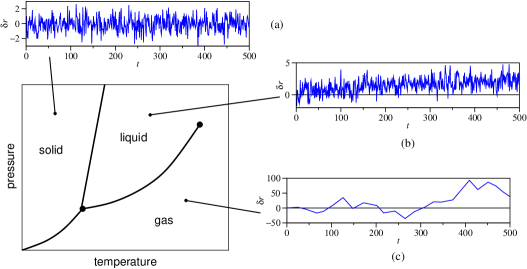
Figure 1: A typical phase diagram showing where the solid, liquid, and gas phases of a substance occurs in the pressure-temperature ($p$-$T$) plane. Also shown in the figure are the equilibrium fluctuations $\delta r$ in the displacement of a given atom in the (a) solid phase, with time-independent variance $\langle(\delta r)^{2}\rangle\propto T$; (b) liquid phase, with a diffusive variance $\langle(\delta r)^{2}\rangle\propto t$; and (c) gas phase, with long ballistic lifetimes.

When the length or time scales of our system of interest are too large, for example, in protein folding (small length scale, but long time scale), or a nuclear weapon detonating in a city (small time scale, but long length scale), or climate change (long length scale and long time scale), it may no longer be possible to identify the order parameters empirically. However, it may be comparatively easy to obtain high-frequency time series data of any number of microscopic quantities. To see how these microscopic time series can be useful towards our elucidation of the phase diagram, we must first understand that each thermodynamic phase is associated with a low-dimensional manifold in the phase space of our system. Such low-dimensional manifolds arise because of conservation laws, or through interaction-driven self-organization, or both. In this statistical mechanical picture, order parameters are the thermodynamic coordinates of individual low-dimensional manifolds. When the system is in a given phase, microscopic variables fluctuate about the associated low-dimensional manifold, which typically has slow dynamics. When the system makes a transition into another phase, the slow dynamics and the low-dimensional manifold changes, and so does the fast fluctuations of the microscopic variables.

In Fig. 1, we illustrate this connection between the character of fast fluctuations and the underlying slow dynamics, by showing the equilibrium fluctuations $\delta r$ in the displacement of a given atom. In Fig. 1(a), we show the non-diffusive equilibrium fluctuations $\delta r$ in the solid phase. In this phase, the variance $\langle(\delta r)^{2}\rangle$ of these fluctuations is proportional to the temperature $T$, but otherwise time independent. In Fig. 1(b), we show the diffusive equilibrium fluctuations $\delta r$ in the liquid phase. In this phase, the variance $\langle(\delta r)^{2}\rangle$ of the fluctuations grows with time. Finally, in Fig. 1(c), we show the diffusive equilibrium fluctuations $\delta r$ in the gas phase. Diffusive fluctuations in the gas phase can be distinguished from those in the liquid phase by the long ballistic lifetimes in the former.

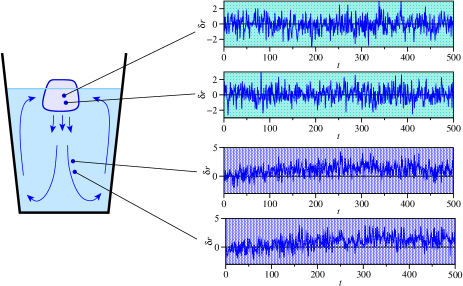
Figure 2: Microscopic time series within a system with mixed phases, in this example, ice and water. Based on our understanding of the character of microscopic fluctuations, the time series can be sorted into an ice cluster and a water cluster. Alternatively, these clusters can be discovered using statistical clustering methods, without any prior knowledge of the phases and their statistical properties.

Now, suppose different phases are present in the system, like the ice-water example shown in Fig. 2. In this example, we can conclude that two phases are present, by sorting the atomic displacement time series into two groups, based on the fluctuation chacracteristics discussed above. Alternatively, we can cluster the microscopic time series, to find the statistically distinct ice and liquid phases. We might even be able to detect the convection currents present in the system. Moreover, if the system undergoes repeated phase transitions, the phases that appear in the history of the system can be discovered by first segmenting the microscopic time series, and then clustering the time series segments. So long as there is adequate data, and the microscopic fluctuations in different phases are sufficiently distinct, we can always discover how many such phases are present through statistical segmentation and clustering of the microscopic time series. These two generally robust procedures are very well suited to the study of complex systems, for which we have high frequency time series data, but no idea how many phases are present, and what their characteristics are. In addition to the macroeconomic study reported in this paper, and related studies on the Japanese economy, the Asian and European economies, we are also applying the two methods to understand protein folding dynamics and earthquake dynamics.

2.3 Segmentation

Financial time series are well known to be highly nonstationary. In particular, several recent studies revealed that the instantaneous volatility fluctuates about a constant level, before switching over rapidly to fluctuations about a different constant level [44, 45, 46]. Based on these, and similar earlier observations, economics and finance practitioners explored various methods for decomposing a nonstationary time series into stationary segments, which are called regimes or trends in the economics and finance literatures. In these literatures, segment boundaries are referred to as structural breaks, trend breaks, or change points. The earliest works in this field are by Goldfeld and Quandt [47], and by Hamilton [48]. Since these pioneering works, an enormous economics literature on structural breaks and change points has been amassed, a few based on the original Markov switching models [49], and many others based on autoregressive models and unit-root tests [50, 51, 52, 53, 54, 55, 56, 57, 58, 59, 60, 61, 62, 63, 64]. In the econophysics literature, apart from our own work, we are aware only of the work by Vaglica et al., who broke the transaction histories of three highly liquid stocks on the Spanish stock market into directional segments to study trading strategies adopted in this market [65], and the recent preprint by Tóth et al., who segmented the time series of market orders on the London Stock Exchange, modeling each segment by a stationary Poisson process [66].

As with all model-driven segmentation of time series data, we assume that each economic sector time series $\mathbf{x}_{i}$ consist of $M_{i}$ segments, and that within segment $m_{i}$, the log-index movements $x^{m_{i}}_{i,t}$ follows a stationary statistical distribution. From the seminal work by Mantegna and Stanley [67], we know that high-frequency index movements can be fitted very well to stable Lévy distributions. We also know from the study by Kullmann et al. [68] that the daily log-index movements can be fitted well to a truncated Lévy distribution, when the sample size is small, but becomes normally distributed when the sample size is large. This suggests that the appropriate model for each stationary segment ought to be a Lévy stable process. However, parameter estimation for Lévy stable distributions [69, 70, 71, 72, 73, 74, 75, 76] is a computationally expensive process, and computing the probability density [77, 78, 79, 80, 81] is equally tedious. From our experience segmenting biological sequences, we know that segment boundaries that are statistically very significant can be discovered by any segmentation procedure, no matter what model we assumed for the underlying stationary segments. We believe that the most statistically significant segment boundaries in financial time series would also be equally insensitive to choice of model, or model mis-specification. Indeed, when we compared segments of the 2002–2003 DJIA half-hourly time series obtained assuming that the log-index movements are normally distributed, against those obtained assuming the log-index movements are Lévy stable distributed, the strongest segment boundaries are in good agreement (no more than two days apart) [82]. With this reassurance, we chose to intentionally mis-specify the model, and work instead with the lognormal index movement model. In this model, the log-index movements in segment $m_{i}$ are assumed to follow a stationary Gaussian process with mean $\mu_{i,m_{i}}$ and variance $\sigma_{i,m_{i}}^{2}$. Unlike parameter estimation for the Lévy distribution, maximum-likelihood estimates of the Gaussian parameters $\mu_{i,m_{i}}$ and $\sigma_{i,m_{i}}^{2}$ can be done very cheaply.

To find the unknown segment boundaries $t_{i,m_{i}}$, which separates segments $m_{i}$ and $m_{i}+1$, we use the recursive segmentation scheme introduced by Bernaola-Galván et al. [24, 25]. In this segmentation scheme, we start with the time series $\mathbf{x}=(x_{1},\dots,x_{t},$ $x_{t+1},\dots,x_{n})$, and compute the Jensen-Shannon divergence [83]

$$\Delta(t)=\ln\frac{L_{2}(t)}{L_{1}},$$ (1)

where within the log-normal index movement model,

$$L_{1}=\prod_{s=1}^{n}\frac{1}{\sqrt{2\pi\sigma^{2}}}\exp\left[-\frac{(x_{s}-\mu)^{2}}{2\sigma^{2}}\right]$$ (2)

is the likelihood that $\mathbf{x}$ is generated probabilistically by a single Gaussian model with mean $\mu$ and variance $\sigma^{2}$, and

$$L_{2}(t)=\prod_{s=1}^{t}\frac{1}{\sqrt{2\pi\sigma_{L}^{2}}}\exp\left[-\frac{(x_{s}-\mu_{L})^{2}}{2\sigma_{L}^{2}}\right]\prod_{s=t+1}^{n}\frac{1}{\sqrt{2\pi\sigma_{R}^{2}}}\exp\left[-\frac{(x_{s}-\mu_{R})^{2}}{2\sigma_{R}^{2}}\right]$$ (3)

is the likelihood that $\mathbf{x}$ is generated by two statistically distinct models: the left segment $\mathbf{x}_{L}=(x_{1},\dots,x_{t})$ by a Gaussian model with mean $\mu_{L}$ and variance $\sigma_{L}^{2}$, and the right segment $\mathbf{x}_{R}=(x_{t+1},\dots,x_{n})$ by a Gaussian model with mean $\mu_{R}$ and variance $\sigma_{R}^{2}$. In terms of the maximum likelihood estimates $\hat{\mu},\hat{\mu}_{L},\hat{\mu}_{R}$ and $\hat{\sigma}^{2},\hat{\sigma}_{L}^{2},\hat{\sigma}_{R}^{2}$, the Jensen-Shannon divergence $\Delta(t)$, which measures how much better a two-segment model fits the time series data compared to a one-segment model, simplifies to

$$\Delta(t)=n\ln\hat{\sigma}-t\ln\hat{\sigma}_{L}-(n-t)\ln\hat{\sigma}_{R}+\frac{1}{2}\geq 0.$$ (4)

Scanning through all possible times $t$, a cut is then placed at $t^{*}$, for which the Jensen-Shannon divergence

$$\Delta^{*}=\Delta(t^{*})=\max_{t}\Delta(t)$$ (5)

is maximized, to break the time series $\mathbf{x}=(x_{1},\dots,x_{n})$ into two statistically most distinct segments $\mathbf{x}^{*}_{L}=(x_{1},\dots,x_{t^{*}})$ and $\mathbf{x}^{*}_{R}=(x_{t^{*}+1},\dots,x_{n})$ (see for example, Fig. 3). This one-into-two segmentation is then applied recursively onto $\mathbf{x}^{*}_{L}$ and $\mathbf{x}^{*}_{R}$ to obtain shorter and shorter segments (see also Fig. 3, for example). At each stage of the recursive segmentation, we also optimize the segment boundaries using the first-order algorithm described in Ref. [84], where we recompute the optimum position of segment boundary $m$, within the time series subsequence bound by segment boundaries $m\pm 1$. This is done iteratively for all segment boundaries, until they have all converged onto their optimum positions.

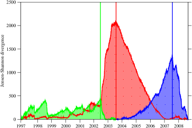
Figure 3: The Jensen-Shannon divergence spectrum for the DJIA time series from Jan 1997 to Aug 2008 (red). This is a typical spectrum consisting of one very strong peak, in this example, at mid-2003. Also show are the Jensen-Shannon divergence spectra for the left segment (green, 1997 to mid-2003) and the right segment (blue, mid-2003 to Aug 2008) obtained at the second stage of the recursive segmentation. In this example, the two segments have divergence maxima at mid-2002 and mid-2007 respectively.

As the optimized recursive segmentation progresses, the Jensen-Shannon divergence of newly discovered segment boundaries, as well as the previously discovered segment boundaries, will in general become smaller and smaller. Segment boundaries thus become less and less significant statistically, and at some point, we must terminate the recursive segmentation. There are three ways to do so. In the first approach, the Jensen-Shannon divergences of new segment boundaries are tested for statistical significance against various $\chi^{2}$ distributions with the appropriate degrees of freedom [24, 25]. The recursive segmentation terminates when no new segment boundaries more significant than the chosen confidence level $p$ can be found. In the second approach, new segment boundaries are accepted if the information criteria of the two-segment models they imply are larger than the information criteria of the one-segment models we are selecting against [85, 86]. Here, the recursive segmentation terminates when further segmentation does not explain the data better. In the third approach, we define signal-to-noise ratios based on the Jensen-Shannon divergence fluctuations within supersegments that new segment boundaries are supposed to divide [84]. The recursive segmentation terminates when the signal-to-noise ratios of all new segment boundaries fall below a chosen threshold value.

Alternatively, we could also terminate the recursive segmentation when no new optimized segment boundaries with Jensen-Shannon divergence greater than a cutoff of $\Delta_{0}=10$ are found. The short and medium segments produced by this termination criterion are reasonable, but the long segments obtained tend to have internal segment structures masked by their context [87]. We then recursively segment these long segments, by progressively lowering the cutoff $\Delta_{0}$ until a segment boundary with strength $\Delta>10$ appears. The final segmentation then consists of segment boundaries discovered through the automated recursive segmentation, as well as segment boundaries discovered through progressive refinement of overly long segments. Based on the experience in our previous works [26, 27], this semi-automatic recursive segmentation appears to produce acceptable results.

2.4 Segment clustering

After the segmentation is completed, we obtain a large number (typically $>100$) of segments for each time series. While successive segments are statistically distinct from each other, segments that are far apart can actually be statistically similar. This observation suggests that the large number of segments make up a small number of segment classes. By comparing multiple indicators, economists classified different market periods into four macroeconomic phases or regimes: (i) a growth phase; (ii) a contraction phase; (iii) a correction phase; and (iv) a crash phase. We therefore expect the time series segments to also be organized into roughly four classes. A similar problem arise in biological sequences, where thousands of segments can be organized into tens of segment types that differ in their biological functions. In the ground-breaking paper by Azad et al., the 248 segments of human chromosome 22 was classified into 53 domain types using single-link hierarchical clustering [88]. Inspired by this prospect of reducing the complexity of our segmentations, we performed independent hierarchical agglomerative clusterings on the segments within each US economic sector time series, using the complete link algorithm (see Ref. [89] for details on the complete link algorithm, and also a review on the broad area of statistical clustering). We chose the complete link algorithm, which is favored by social scientists for producing compact and internally homogeneous clusters [90], because our goal is to discover macroeconomic phases with well-defined statistical properties. We do not use the far more popular single link algorithm [91, 92], because it tends to produce loose and elongated clusters [93]. Single link clustering is more meaningful in the biological sciences, generating phylogenetic trees for example, because the clustering procedure corresponds more closely with the nature of evolutionary changes. In general, if one expects to find highly homogeneous collections of objects one would use complete link clustering, whereas if one expects to find collections of objects that evolved from common ancestors one would use single link clustering.

Figure 4: The complete-link hierarchical clustering tree for the time series segments of the Dow Jones Industrial Average between January 1997 and August 2008. In this tree, we show the Jensen-Shannon divergence values at which the top branches diverge. We also show how uniform thresholds can be selected to break the tree into two, three, four, or six clusters. Finally, we show how individual thresholds can be selected to obtain the six clusters reported in Ref. [26], which are colored in increasing order of market volatility as deep blue, blue, green, yellow, orange, and red.

In this segment clustering, we used the Jensen-Shannon divergences between segments as their statistical distances. Clustering of different periods within a financial time series has been previously investigated [94, 95, 96], in the absence of any segmentation analysis. After complete-link hierarchical clustering of the segments within a given time series, we typically end up with a dendrogram like that shown in Fig. 4 for the Dow Jones Industrial Average. By varying a uniform threshold, different number of clusters can be identified. A small number of clusters provide a coarser description, whereas a larger number of clusters offer a finer description of the dynamics within the time series. This different numbers of clusters form a nested hierarchy of coarse-grained descriptions of the US macroeconomic dynamics. All these descriptions are correct, but some are more useful than others, because they are statistically more robust. For example, in Fig. 4, we can identify four clusters if the uniform threshold is $42.7<\Delta<102.2$, or five clusters if the uniform threshold is $34.4<\Delta<42.7$, or six clusters if the uniform threshold is $31.3<\Delta<34.4$. Because of the broader range of uniform thresholds, a four-cluster description is statistically more robust than a five-cluster or six-cluster descriptions of the time series segments.

Once we understand statistical robustness as the primary criterion for cluster selection, we can also employ local thresholds for each cluster. In Fig. 4, we show as an example the local thresholds used to pick six clusters. Other local thresholds can also be used, but so long as they are statistically robust, one choice of clusters offer no advantage over another choice of clusters. These different choices of clusters tell the same story, merely with different contrasts, very much like red-tinted and blue-tinted versions of the same photograph. With this in mind, we analyzed the hierarchical complete-link clustering trees obtained for all ten DJUS economic sectors, and selected between four to six clusters of segments for each US economic sector. These clusters represent different macroeconomic phases (differentiated by their market volatilities) present in the time series data. Once all segments have been assigned to their respective clusters, we use the heat-map-like color scheme in Table 2 to plot the temporal distributions of clustered segments. All the analyses presented in this paper are based on features identified from the temporal distributions of clustered segments for the ten DJUS economic sector indices.

Table 2: Heat-map-like color scheme for the different volatility clusters, and the macroeconomic phases they correspond to. The crisis phase, which consists of the high-volatility (yellow) and very-high-volatility (orange) clusters, is significantly longer than the economic contraction phase accepted by economists. In fact, economic contraction, as determined by successive quarters of contraction in the GDP, typically occurs at the end of a crisis phase. Also shown are the average standard deviation in each phase for the various economic sectors. The extremely-low-volatility phase is seen only in CY, EN, and FN, because the time series segments are organized into six clusters for these three sectors only. As we can see, within each macroeconomic phase, the average volatilities discovered by the clustering procedure are fairly consistent throughout most sectors. The exceptions are HC and TL, which have consistently lower volatilities. It is possible to introduce a seventh cluster with volatility $\sigma\approx 0.008$, and have all the clusters reclassified. This will produce a deterministic mapping between volatility and color, but we choose not to, so as to achieve maximum visual contrast with the present color scheme.

volatility	extremely low	low	moderate	high	very high	extremely high
color	black	blue	green	yellow	orange	red
phase	growth		correction	crisis		crash
BM	-	0.0016	0.0037	0.0046	0.0069	0.0146
CY	0.0005	0.0015	0.0023	0.0031	0.0053	0.0121
EN	0.0010	0.0014	0.0027	0.0037	0.0058	0.0152
FN	0.0007	0.0016	0.0024	0.0039	0.0058	0.0134
HC	-	0.0006	0.0016	0.0023	0.0041	0.0076
IN	-	0.0013	0.0022	0.0035	0.0056	0.0140
NC	-	0.0009	0.0015	0.0022	0.0034	0.0085
TC	-	0.0019	0.0030	0.0042	0.0082	0.0121
TL	-	0.0008	0.0018	0.0024	0.0033	0.0078
UT	-	0.0014	0.0023	0.0030	0.0038	0.0088

2.5 Identifying corresponding segments

Of the many features that we can identify from individual temporal distributions, as well as across the panel of temporal distributions, corresponding segments that appear in all or most of the indices are the most striking visually. In the economics and finance literature, a mean or volatility movement that occurs over multiple time series is called comovement [97, 98, 99, 100, 101, 102, 103], common jumps [104, 105, 106], common shocks [107, 108, 109], or common breaks [110, 111, 112, 113, 114, 115]. The consensus that arise from this body of work is that the statistical significance of a change point is amplified by the cross section it occurs concurrently over.

In our study, the corresponding segments do not necessarily start at the same time, because our use of high-frequency data allows us to identify the change points that are individually optimum for the ten DJUS economic sector indices. More importantly, our corresponding segments in the various indices do not end at the same time. As discussed in Ref. [27], the durations of each corresponding segment, and the Jensen-Shannon divergence values at the start of these segments, tell us how strongly the shock impacted different sectors in the US economy. Moreover, the different start times of the corresponding segments allow us to roughly map out the progress of the shock.

Because of the different start times and different durations, we mark segments in the ten DJUS economic sector indices as corresponding segments if they (i) have similar volatilities (high and high, or low and low); or (ii) are flanked by volatility movements in the same directions(low-to-high and moderate-to-high, or high-to-low and moderate-to-low). For this, we took advantage of the heat-map-like color scheme in the temporal distributions.

2.6 Cross-correlations

In performing segmentation and thereafter segment clustering, we have selectively discarded information contained in the ten high-frequency time series to obtain a coarse-grained picture of the US macroeconomic dynamics. While this picture provides a useful bird’s eye view of the dynamical processes within the US economy, a significant amount of useful information has also been thrown out. To recover more of the information contained in the high-frequency time series, and shed more light on the exciting stories unfolding before our eyes, we compute the normalized cross-correlation matrix $C$, whereby the matrix element

$$C_{ij}=\frac{\sum_{t=1}^{T}(x_{it}-\bar{x}_{i})(x_{jt}-\bar{x}_{j})}{\sqrt{\sum_{t=1}^{T}(x_{it}-\bar{x}_{i})^{2}\sum_{t^{\prime}=1}^{T}(x_{jt}-\bar{x}_{j})^{2}}}$$ (6)

is the zero-lag cross-correlation between US economic sectors $i$ and $j$.

Cross-correlations between different stocks, and between different benchmark indices have been widely studied in the finance literature. Such studies have been particularly popular in the bid to understand the meltdown of global financial markets during the present financial crisis [117, 118, 119, 120, 121, 122]. In the econophysics literature, there have been attempts to understand the nontrivial cross-correlations between different financial time series using random matrix theory [123, 124, 125, 126, 127, 128, 129, 130]. In all these studies, the cross-correlations were computed either over the entire data period, or over sliding windows. In our own study, we not only calculate the cross-correlation matrix over the entire duration of the time series, but also over two-year intervals strictly within the growth and crisis macroeconomic phases, and over individual corresponding segments.

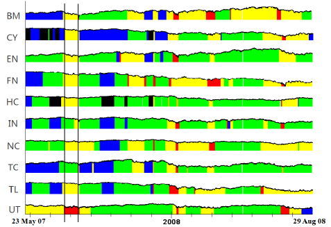
Figure 5: Interval selected for the computation of the cross-correlation matrix between the ten DJUS economic sector indices. In this figure, the lower and upper limits of the interval are chosen such that the interval covers a single macroeconomic phase for nearly all indices. Exception is made for IN, because its high-volatility segment is too short, and thus the selected interval also covers the preceding moderate-volatility segment.

To compute the cross-correlation matrix over a given corresponding segment, we select the largest interval within which most sectors can be found in a single macroeconomic phase, as shown in Fig. 5. For the primarily high-volatility corresponding segment identified in Fig. 5, the start dates and end dates in the different sectors are shown in Table 3. Based on these dates, we chose our interval to start on July 25, 2007, and end on August 14, 2007, so that all DJUS economic sectors, with the exception of IN, TC, and UT, are strictly in the high-volatility phase. Within this interval, UT is strictly in the extremely-high-volatility phase. The selected high-volatility interval overlaps with the moderate-volatility phases in IN and TC. This cannot be helped, because the high-volatility phases in IN and TC started so late. Furthermore, we believe it is meaningful to allow this overlap, because the start dates of the moderate-volatility segments in IN and TC are very close to the start dates of the high-volatility segments in the other sectors.

Table 3: Start dates and end dates in different DJUS economic sectors for the primarily high-volatility corresponding segment identified in Fig. 5. The high-volatility segments for IN and TC started significantly later than those in other sectors, so we also show the start and end dates for the preceding moderate-volatility segments for these two sectors. For UT, it is a extremely-high-volatility segment that coincides with the high-volatility segment in other sectors.

Economic Sector	Start Date	End Date
BM	July 23, 2007	August 14, 2007
CY	July 25, 2007	August 16, 2007
EN	July 23, 2007	August 15, 2007
FN	July 23, 2007	August 15, 2007
HC	July 20, 2007	August 15, 2007
IN	July 19, 2007	August 7, 2007
	August 8, 2007	August 16, 2007
NC	July 25, 2007	September 9, 2007
TC	July 17, 2007	August 14, 2007
	August 15, 2007	August 16, 2007
TL	July 20, 2007	August 16, 2007
UT	July 24, 2007	August 16, 2007

In Table 4, we show the cross-correlation matrix computed using (a) this optimum interval, such that apart from IN and TC, all sectors are in the high-volatility or extremely-high-volatility phases. To show that the criterion we used to select interval (a) produce statistically robust cross correlations, we compare them against cross correlations computed using the intervals (b) and (c). Interval (b) is four trading days shorter than interval (a), with two trading days taken off the latter’s start and end. As with interval (a), all sectors apart from IN and TC are in the high-volatility or extremely-high-volatility phases within this interval. In contrast, interval (c) is four trading days longer than interval (a), with two trading days added to the latter’s start and end. Unlike for intervals (a) and (b), cross correlations computed within this longer interval will contain contributions from the lower-volatility phases adjacent to the high-volatility corresponding segment for nearly all sectors. As we can see from Table 4, the maximum positive difference between cross correlations in (b) and cross correlations in (a) is $+0.063$, occurring for CY-TL, and the maximum negative difference between cross correlations in (b) and cross correlations in (a) is $-0.029$, occurring for HC-EN. Similarly, the maximum positive difference and maximum negative difference between cross correlations in (c) and cross correlations in (a) is $+0.041$ and $-0.072$, occurring for HC-EN and BM-FN, respectively. The differences in cross correlations is generally larger for the longer interval (c) than for the shorter interval (b), because in (b), the interval contains a single statistically stationary segment for most sectors, whereas in (c), the interval incorporated time series data from more than one segments. Nonetheless, these cross correlational differences are all small.

Table 4: Cross-correlation matrix computed from the half-hourly times series of the ten DJUS economic sector indices over three intervals: (a) from July 25, 2007 to August 14, 2007; (b) from July 27, 2007 to August 10, 2007; and (c) from July 23, 2007 to August 16, 2007.

(a) BM CY EN FN HC IN NC TC TL UT BM 0.872 0.825 0.898 0.726 0.900 0.789 0.818 0.709 0.832 CY 0.872 0.753 0.898 0.826 0.915 0.876 0.856 0.768 0.835 EN 0.825 0.753 0.750 0.663 0.776 0.720 0.745 0.607 0.759 FN 0.898 0.898 0.750 0.771 0.889 0.845 0.827 0.741 0.814 HC 0.726 0.826 0.663 0.771 0.827 0.913 0.804 0.772 0.770 IN 0.900 0.915 0.776 0.889 0.827 0.861 0.877 0.808 0.842 NC 0.788 0.876 0.720 0.845 0.913 0.861 0.852 0.783 0.819 TC 0.818 0.856 0.745 0.827 0.804 0.877 0.852 0.769 0.783 TL 0.709 0.768 0.607 0.741 0.772 0.808 0.783 0.769 0.729 UT 0.832 0.835 0.759 0.814 0.770 0.842 0.819 0.783 0.729 (b) BM CY EN FN HC IN NC TC TL UT BM 0.888 0.807 0.891 0.713 0.909 0.783 0.843 0.746 0.823 CY 0.888 0.752 0.928 0.848 0.932 0.910 0.904 0.831 0.859 EN 0.807 0.752 0.728 0.634 0.771 0.703 0.747 0.619 0.736 FN 0.891 0.928 0.728 0.770 0.894 0.849 0.849 0.770 0.808 HC 0.713 0.848 0.634 0.770 0.826 0.921 0.793 0.784 0.772 IN 0.909 0.932 0.771 0.894 0.826 0.880 0.880 0.830 0.847 NC 0.783 0.910 0.703 0.849 0.921 0.880 0.865 0.816 0.838 TC 0.843 0.904 0.747 0.849 0.793 0.880 0.865 0.764 0.802 TL 0.746 0.831 0.619 0.770 0.784 0.830 0.816 0.764 0.768 UT 0.823 0.859 0.736 0.808 0.772 0.847 0.838 0.802 0.768 (c) BM CY EN FN HC IN NC TC TL UT BM 0.837 0.835 0.826 0.738 0.912 0.770 0.840 0.705 0.821 CY 0.837 0.771 0.891 0.847 0.906 0.891 0.868 0.787 0.844 EN 0.835 0.771 0.743 0.704 0.802 0.736 0.775 0.639 0.783 FN 0.826 0.891 0.743 0.785 0.860 0.853 0.824 0.737 0.804 HC 0.738 0.847 0.704 0.785 0.842 0.914 0.829 0.784 0.793 IN 0.912 0.906 0.802 0.860 0.842 0.860 0.902 0.808 0.838 NC 0.770 0.891 0.736 0.853 0.914 0.860 0.868 0.792 0.826 TC 0.840 0.868 0.775 0.824 0.829 0.902 0.868 0.785 0.796 TL 0.705 0.787 0.639 0.737 0.784 0.808 0.792 0.785 0.746 UT 0.821 0.844 0.783 0.804 0.793 0.838 0.826 0.796 0.746

To understand what impacts these small cross correlational differences have on the minimal spanning trees (described in the next subsection) we generate for this study, we show in Fig. 6 the minimal spanning trees derived from the cross-correlation matrices for these three intervals. In this figure, we see the same EN-BM-IN-CY-NC-HC backbone, which is insensitive to how we select the interval, and thus statistically robust. We also see that the sectors TC, TL, and UT, are linked sometimes to IN, and other times to CY. Going back to the cross correlations shown in Table 4 between TC, TL, UT and CY, IN, we find poor agreements over the three intervals for the CY-TC, CY-TL and CY-UT cross correlations. In contrast, the IN-TC, IN-TL, and IN-UT cross correlations are in good agreement over the three intervals. This suggests that the minimal spanning links between TC, TL, UT and CY, IN are not as statistically robust as the rest of the minimal spanning links in this corresponding segment. In any case, we shall see in Section 3 that CY and IN are core sectors, while TC, TL, and UT are fringe domestic sectors of the US economy. Whether they are to IN or CY, minimal spanning links directly connect TC, TL, UT from the fringe to CY, IN in the core. This direct core-fringe linkage in itself represents a statistically robust characteristic of the US economy.

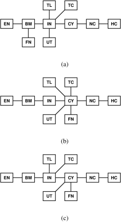
Figure 6: The minimal spanning trees of the ten DJUS economic sectors, constructed using half-hourly time series from (a) July 25, 2007 to August 14, 2007; (b) July 27, 2007 to August 10, 2007; and (c) July 23, 2007 to August 16, 2007.

2.7 Minimal spanning trees

Even though our cross-correlation matrices are only $10\times 10$ in size, the information contained in the 36 independent matrix elements is still not easy for a human to process. To better understand the correlational dynamics between the US economic sectors at different times, we look instead at simplified graphical representations of the cross-correlation matrices. For this study, we work primarily with the minimal spanning tree (MST) representation of the cross-correlation matrix. In Section 4.3, We also also explore the planar maximally filtered graph (PMFG) representation, to understand what kind of cross-correlational structures have been left out in the MST representation, in which cycles are not admitted. Ultimately, if we had analyzed the cross correlations network of all stocks on the American stock markets, community detection methods [131, 132, 133, 134, 135, 136, 137] will allow us to develop a coarse grain description of the US economy, and thereby shed more light on its dynamics. In this study, the use of such techniques are not necessary, since we are only looking at ten DJUS economic sector indices, which are themselves already coarse grain descriptions of the US markets.

The minimal spanning tree (also called minimum spanning tree) approach to understanding weighted graphs is frequently credited to Kruskal [138] or Prim [139], although there were studies dating all the way back to 1926. For a good reading on the history of the minimal spanning tree method, see the article by Graham and Hell [140]. In economics, the method is not widely used [141, 142]. However, since its first application in econophysics by Mantegna [143], and shown to be a robust caricature of the underlying correlations [144, 145], the MST has been incorporated into the basic tool suite for statistical analysis of financial market data [146, 147, 148, 149, 150, 151, 152]. In particular, Onnela et al. made extensive use of MSTs to study the dynamics of cross correlations during market crashes [153, 154, 155]. Clustering techniques based on the MST have also been used to discover different sectors in a stock market [156, 157, 158, 159, 160, 161], how the interdependences of the European economies are evolving [162, 163], and how global markets are linked to each other [164, 165, 166]. More recently, Eom et al. used the MST as a means to reduce the $N(N-1)/2$ linkages between $N$ stocks to $N-1$ links, for studying the effects of market factors on the information flow between stocks [167].

To construct an MST representation of the cross-correlation matrix, Mantegna defined the distance metric [143]

$$d_{ij}=\sqrt{2(1-C_{ij})},$$ (7)

which measures the statistical distance between two financial time series $i$ and $i$, whose cross-correlation is $-1\leq C_{ij}\leq 1$. Applying Kruskal’s algorithm [138], a link is first drawn connecting the pair $(i_{1},j_{1})$ of time series with the smallest distance $d_{i_{1}j_{1}}=\min_{(i,j)}d_{ij}$. Following this, a link is drawn connecting the pair $(i_{2},j_{2})$ with the next smallest distance $d_{i_{2}j_{2}}=\min_{(i,j)\neq(i_{1},j_{1})}d_{ij}$. This process is repeated with pairs $(i_{k},j_{k})$ with increasingly larger distances $d_{i_{k}j_{k}}$, until all time series are incorporated into the spanning graph. There is one additional constraint: if $(i_{l},j_{l})$ is the next pair of time series to be linked based on their distance $d_{i_{l}j_{l}}$, but will create a cycle in the growing graph in so doing, no link will be drawn between $i_{l}$ and $j_{l}$. Instead, we will skip $(i_{l},j_{l})$ and move on to the pair $(i_{m},j_{m})$ with the next smallest distance $d_{i_{m}j_{m}}$. The spanning graph obtained at the end contains no cycles, hence the name minimal spanning tree. Alternatively, since $d_{ij}$ is a monotonically decreasing function of $C_{ij}$, we can get the same MST, if we start by linking the pair of time series with the largest cross-correlation, and then progressively linking pairs with smaller and smaller cross-correlations, so long as we ensure the no-cycle constraint is satisfied at all times.

3 Macroeconomic MSTs

Before we move on to our MST analysis, let us first develop an intuitive picture for the sectorial structure of the US economy. As a significant fraction of what the US produces is consumed domestically, the US market is a gigantic consumption market. We therefore expect the noncyclical consumer goods (NC) and consumer services (CY) to be central players in the US economy. Furthermore, CY and NC consume products predominantly generated by the industrials (IN), thus we expect IN, CY and NC (and perhaps also FN, since financing is an important ingredient in US consumerism) to be the core sectors of the US economy. In contrast, emerging economic sectors such as telecommunications (TL) and technologies (TC), along with less attractive economic sectors like healthcare (HC) and utilities (UT), contribute less significantly to the GDP, and hence sit at the fringe of the US economy. Finally, the oil & gas (EN) and basic materials (BM) sectors are strongly driven by changes in the global supply and demand cycle, and thus represent the US economy’s connection to the global market.

Indeed, this intuitive picture is supported by quantitative GDP data from the US Bureau of Economic Analysis (BEA) [168]. The BEA uses an industry classification scheme different from the ICB, so we map the BEA data onto the ICB economic sectors using the subindustry descriptions available, as shown in Table 5, to figure out what their GDP contributions are. Though somewhat overestimated because of this mapping problem, we see that CY, IN, and NC combined contributed on average about 7,000 billion USD to the US gross domestic product (GDP), which was worth 14,200 billion USD on average between 2007 and 2009. These three sectors therefore contribute about 50% of the US GDP. FN, by itself, contributed about 3,000 billion USD to the US GDP, or about 21%. These contributions support our intuitive picture of these four sectors playing a central role in the US economy. Based on the subindustry breakdown in Table 5, HC probably contributes on average slightly more than 1,000 billion USD to the US economy annually, or about 7% of the GDP. The contributions from TC and TL are hard to nail down, because their subindustries are frequently lump with others that are assigned to CY, but we estimate that their contributions to the GDP are around the 300 billion USD mark, or about 3% of the GDP. From Table 5, we see that UT contributes 260 billion USD (about 2%) on average annually, while BM and EN both contribute around the 400 billion USD mark, also around 3%, to the US GDP. Again, based on these numbers, we are probably not too far off guessing that these sectors are less critical to the US economy.

Table 5: Contributions in billions of USD to the US gross domestic product (GDP) by the various Bureau of Economic Analysis (BEA) industries for 2007, 2008, and 2009. The industry classification used by the BEA differs from the ICB. While some BEA industries can be easily assigned to a unique DJUS economic sector, other BEA industries contain subindustries from more than one DJUS economic sector. A BEA industry is marked with a dagger, if we assign it to one economic sector, but some of its listed subindustries to other economic sectors. In these cases, the GDP contributions will be split between the economic sectors. On the other hand, if its subindustries belong to different economic sectors, but are not finely divided enough for us to split its GDP contributions, the BEA industry will be marked with an asterix. For BEA industries with mixed components in CY, IN, and NC, we do not break the GDP contributions down by subindustries. Data taken from Ref. [168].

Industry			2007	2008	2009	Economic Sector
Gross domestic product			14,061.8	14,369.1	14,119.0
Private industries			12,301.9	12,514.0	12,196.5
	Agriculture, forestry, fishing, and hunting*		144.7	160.1	133.1	NC
	Mining†		91.3	106.3	99.1	BM
		Oil and gas extraction	162.9	210.8	141.7	EN
	Utilities		248.8	262.6	268.1	UT
	Construction		657.2	623.4	537.5	IN/NC
	Manufacturing†		1,138.9	1,119.9	1,092.1	IN/NC
		Primary metals	59.0	61.5	43.4	BM
		Paper products	58.6	53.8	56.1	BM
		Petroleum and coal products	149.7	151.9	120.0	EN
		Chemical products	223.2	201.1	216.5	BM/HC
		Plastics and rubber products	69.5	59.4	56.7	BM
	Wholesale trade		813.3	822.9	780.8	CY
	Retail trade		886.1	840.2	819.6	CY
	Transportation and warehousing		405.4	418.7	389.5	IN/CY
	Information*†		285.6	293.4	283.5	CY
		Broadcasting and telecommunications	347.7	359.1	355.8	TL
	Finance, insurance, real estate, rental, and leasing		2,891.3	2,974.9	3,040.3	FN
	Professional and business services		1,700.5	1,768.8	1,701.3	CY/IN
	Educational services, health care, and social assistance		1,078.3	1,148.9	1,212.9
		Health care and social assistance	941.0	1,001.9	1,057.9	HC
	Arts, entertainment, recreation, accommodation, and food services		545.2	535.4	513.1	CY
	Other services, except government		344.6	340.9	335.4	CY
Government			1,759.9	1,855.1	1,922.5

Table 6: Cross-correlation matrix computed from the half-hourly time series of the ten DJUS economic sector indices over the period February 2000 to August 2008. Also shown are the cross correlations $\langle C\rangle$ of each economic sector averaged across the rest of the US economy.

	BM	CY	EN	FN	HC	IN	NC	TC	TL	UT
BM		0.611	0.522	0.568	0.347	0.656	0.556	0.438	0.435	0.458
CY	0.611		0.320	0.767	0.435	0.815	0.660	0.679	0.600	0.433
EN	0.522	0.320		0.316	0.261	0.393	0.350	0.254	0.276	0.451
FN	0.568	0.767	0.316		0.403	0.751	0.616	0.577	0.559	0.440
HC	0.347	0.435	0.261	0.403		0.436	0.469	0.325	0.342	0.323
IN	0.656	0.815	0.393	0.751	0.436		0.660	0.775	0.618	0.445
NC	0.556	0.660	0.350	0.616	0.469	0.660		0.472	0.497	0.485
TC	0.438	0.679	0.254	0.577	0.325	0.775	0.472		0.566	0.270
TL	0.435	0.600	0.276	0.559	0.342	0.618	0.497	0.566		0.382
UT	0.458	0.433	0.451	0.440	0.323	0.445	0.485	0.270	0.382
$\langle C\rangle$	0.510	0.591	0.349	0.555	0.371	0.617	0.529	0.484	0.475	0.410

To further verify our intuitive picture of the US economy, we computed the cross-correlation matrix of the time series from February 2000 to August 2008. As shown in Table 6, IN and CY are the most strongly correlated, with $C(\rm IN,CY)=0.815$, while EN and TC are the least strongly correlated, with $C(\rm EN,TC)=0.254$. Based on the average cross correlations $\langle C\rangle$, it also appears that IN is most strongly tied in with the rest of the sectors ($\langle C\rangle(\rm IN)=0.617$), while EN is least strongly tied in with the rest of the US economy ($\langle C\rangle(\rm EN)=0.349$). Based on this cross-correlation matrix, we constructed the MST shown in Fig. 7(a). As expected, the core sectors of the US economy, IN, CY and NC, are at the centre of the MST. The sectors EN and BM, which represent the US economy’s connection to the world market, sit on one end of the MST, while the sectors HC, TC, TL, and UT, lies on the fringe of the MST, consistent with their lesser importance to the US economy. Heimo et al. arrived at a similar conclusion, in their MST study of 116 NYSE stocks from 1982 to 2000 [169].

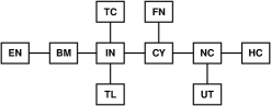
(a)
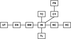
(b)
(c)

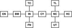
(d)

Figure 7: The MSTs of the ten DJUS economic sectors, constructed using half-hourly time series from (a) February 2000 to August 2008, (b) 2001–2002, (c) 2004–2005, and (d) 2008-2009. The first and the third two-year windows, (b) and (d), are entirely within an economic crisis, whereas the second two-year window, (c), is entirely within an economic growth period.

Over the period 2000 to 2009, the US National Bureau of Economic Research (NBER) recorded two economic contractions [170]. The first was from March 2001 to November 2001. The second was from December 2007 to June 2009. Our own studies showed that the US economy went from a crisis phase (mid-1998 to mid-2003, which contained the March 2001 to November 2001 contraction) into a growth phase (mid-2003 to mid-2007), and back into a crisis phase (mid-2007 to present, which contained the December 2007 to June 2009 contraction) [26]. We expect interesting structural differences between the MSTs constructed entirely within the previous crisis (2001–2002, Fig. 7(b)), the previous growth (2004–2005, Fig. 7(c)), and the present crisis (2008–2009, Fig. 7(d)). Indeed, we see two topologically distinct MST structures: a chain-like MST structure which occurs for both crises, and a star-like MST structure which occurs for the growth phase. Even though we only have three data points (two crises and a growth), we believe the generic association of chain-like MST and star-like MST to the crisis and growth phases respectively is statistically robust. Our reasons are two-fold. First, the MST is a representation based on order statistics (ranks of cross correlations). Results derived based on order statistics, which are insensitive to noise, tend to be highly robust statistically, as we have illustrated in Section 2.6. Second, the star-to-chain transition in the MST structure as the US economy goes from growth into crisis cannot be brought about by a fixed quantum increase, nor can it be caused by a proportional increase, in correlations. These two types of correlational changes do not change the ordering of cross correlations among the ten economic sectors, and hence cannot modify the MST.

Since noise and global shifts in correlations cannot be responsible for the star-to-chain or the chain-to-star transitions, correlational changes that accompany these transitions must be highly significant. Our assessment that the topology change in the MST is statistically significant is further supported by the observations by Onnela et al., who looked at the mean occupation level around the most connected node in their MST, and found the mean occupation level becoming low during market crashes [153, 154, 155]. This is the same phenomenon we see for the star-to-chain evolution, at the microscopic scale of individual stocks. In the next two sections, we will investigate the characters of these correlational changes, and discuss the implications for early detection of true economic recovery based on the chain-to-star transition.

From Fig. 7, we also see that in both the crisis and growth phases, IN is found be the central industry of the US economy. This is understandable, since the United States is a highly industrialised country with IN driving the rest of the sectors. However, when the US economy went from the mid-2003 to mid-2007 economic growth into the current crisis, the IN star center shed the sectors NC, HC and TL, which shifted to other parts of the MST. In the restructured MST, NC formed the center of another cluster. We believe this is a signature of the trigger role played by NC in the Subprime Crisis, since homebuilders and developers (who are most directly affected by the waves of mortgage defaults) are classified under this economic sector. More interestingly, the cluster centered around NC consists of HC, TL, and UT, which were part of the five sectors that went first into the crisis phase (see Fig. 5 in Ref. [27]). The last of these five sectors is IN, so it appears that correlational changes within these five sectors in July 2007 is responsible for the main difference between the growth MST (Fig. 7(c)) and the crisis MST (Fig. 7(d)). This gross restructuring of the MST thus provides an interesting way to visualize how the current financial crisis propagated throughout the entire US economy.

4 Segment-by-segment analysis

Even within the macroeconomic growth and crisis phases, the DJUS economic sector time series are highly nonstationary. Both the cross correlations between the ten sectors, and the MSTs they imply, are expected to be highly dynamic. To understand how cross correlations change with time, we extracted the average cross correlations of the ten DJUS economic sectors in 11 corresponding segments within the present financial crisis (see Fig. 8). All four macroeconomic phases are represented in these 11 corresponding segments. Ranking the average cross correlations from highest to lowest in Table 7, we see that IN is always most strongly correlated to the rest of the US economy, whatever the prevailing economic climate, followed by CY and NC. Meanwhile, EN is most weakly coupled to the rest of the US economy, in most of the corresponding segments. This is consistent with our expectation that the oil & gas industry’s strong dependence on global supply and demand makes it less susceptible to movements within the US economy.

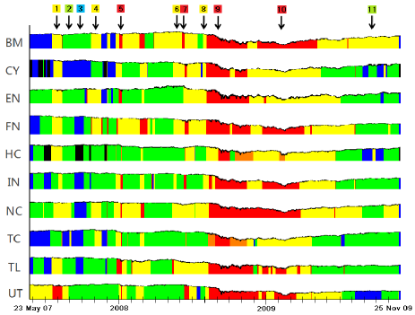
Figure 8: Eleven corresponding segments identified in the time series of the ten DJUS economic sector indices after the mid-2007 onset of the present global financial crisis. In this figure, the corresponding segments are numbered from ‘1’ to ‘11’. In the rest of the paper, we label these corresponding segments by their dominant volatility, and then by their order of appearance, so that ‘1’ = Y1, ’2’ = G1, ’3’ = B, ’4’ = Y2, ’5’ = R1, ’6’ = Y3, ’7’ = R2, ’8’ = Y4, ’9’ = R3, ‘10’ = R4, ‘11’ = G2. Note that Y1 is the same corresponding segment identified in Fig. 5, where we show the temporal distributions of clustered segments of the ten DJUS economic sectors from May 23, 2007 to August 29, 2008, instead of from May 23, 2007 to November 25, 2009 in this figure.

Table 7: Ranks of the ten DJUS economic sectors based on their average half-hourly cross-correlations, over February 2000 to November 2009, as well as over the 11 corresponding segments identified in Fig. 8. The average cross correlations for EN in Y3, and those for BM, EN, and UT in Y4, are anomalously low, even negative. Also shown are the cross correlations $\langle\!\langle C\rangle\!\rangle$ averaged over all ten sectors, for the entire period from February 2000 to November 2009, as well as the 11 corresponding segments.

	BM	CY	EN	FN	HC	IN	NC	TC	TL	UT	$\langle\!\langle C\rangle\!\rangle$
Entire	5	2	10	3	9	1	4	6	7	8	0.489
Y1	6	2	10	4	8	1	3	5	9	7	0.811
G1	6	2	10	5	7	1	3	4	9	8	0.738
B	2	8	10	7	4	1	3	5	9	6	0.511
Y2	4	3	10	8	6	1	2	5	7	9	0.700
R1	7	9	3	10	8	1	2	4	5	6	0.797
Y3	9	2	10	7	4	1	5	3	6	8	0.562
R2	7	3	10	2	8	1	6	9	4	5	0.703
Y4	9	4	10	2	5	1	7	3	6	8	0.559
R3	5	2	10	10	4	1	3	6	9	8	0.863
R4	4	3	5	7	6	2	1	8	10	9	0.796
G2	4	2	6	7	9	1	5	3	10	8	0.709

In general, we observe a positive correlation between the average market cross correlation $\langle\!\langle C\rangle\!\rangle$ and the market volatility. As can be seen from Table 7, higher average market cross correlations are generally associated with higher volatility phases. Specifically, in the low-volatility economic growth phase (B), the average market cross correlation is low, in the range $0.5<\langle\!\langle C\rangle\!\rangle<0.6$, whereas in the moderate-volatility market correction phase (G1, G2), the average market cross correlation is also moderate, in the range $0.6<\langle\!\langle C\rangle\!\rangle<0.7$. In the higher-volatility phases (Y1, Y2, Y3, Y4; R1, R2, R3, R4), the average market cross correlation is high, in the range $0.7<\langle\!\langle C\rangle\!\rangle<0.9$. The higher correlations observed during the higher-volatility phases is consistent with the tendency for traders to panic and to buy and sell stocks from different sectors at the same time. Conversely, when the market is calm, stocks from different sectors tend to be bought and sold at different times, explaining the lower correlations observed for the lower-volatility phases. These average market cross correlations are all higher than the average market cross correlations computed over the entire time series, because cross correlations within the US economy has been increasing over the years (see for example, Ref. [171]).

4.1 MST structures

As expected, changes in the MST can be seen going from one corresponding segment to the next (see Fig. 9). However, the sectors IN, CY and NC remain at the cores of all 11 MSTs, whereas the sectors HC, TC, TL, and UT are mostly found at the fringes of these MSTs. Interestingly, the financials (FN), which is frequently found close to the core, occasionally drifts out to the fringe. While the core-and-fringe structure of the MSTs remains well defined as the market volatility changes, we observe shifting relative importances between the different sectors. We wll study these MST rearrangements, which we believe are the US economy’s response to shocks originating within specific economic sectors, in Section 5. Here, let us make the remarkable observation that, through the fluxes of correlational changes, the EN-BM-IN-CY-NC-TC-HC backbone of the MSTs remained relatively unchanged throughout the entire crisis period. This robust correlational structure must therefore be a key to understanding the performance of the present US economy.

In Fig. 9, we incorporate more visual information on the cross-correlation matrix, by varying the widths of the bonds in the MSTs. The thicker the bond between two sectors, the stronger their correlations. As we can then see, sectors at the core are generally more strongly correlated than those on the fringes of the MSTs. This reinforces our intuitive picture that sectors on the fringe are more detached from the overall economy, whereas those at the core are most important to the US economy. In this representation of the MSTs, a correlational core consisting of thick bonds can also be seen. Even as the core and backbone of the MSTs remain more or less unchanged, the correlational core of thick bonds expands and contracts with time. We can think of the correlational core defining the active participants in the US economy for a given corresponding segment. In the high-volatility phase, the correlational core expands all the way out to the fringes, telling us that fringe sectors become more involved in the US economy during a financial crisis. A similar phenomenon was observed by Onnela et al. in the MSTs of individual stocks across market crashes [153, 154, 155].

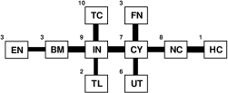
(a)

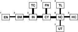
(b)

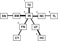
(c)

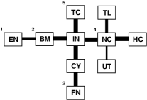
(d)

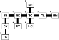
(e)

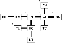
(f)

Figure 9: MSTs of the ten DJUS economic sectors for the corresponding segments (a) Y1, (b) G1, (c) B, (d) Y2, (e) R1, (f) Y3, (g) R2, (h) Y4, (i) R3, (j) R4, (k) G2, within the present financial crisis. In this figure, thicker bonds represent stronger cross correlations, whereas the number besides each sector indicates the order with which the sector made the transition into the given corresponding segment (whereever they can be identified).

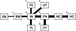
(g)

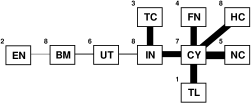
(h)

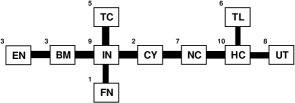
(i)
(j)
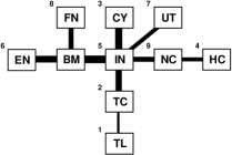
(k)

Figure 9: (continued) MSTs of the ten DJUS economic sectors for the corresponding segments (a) Y1, (b) G1, (c) B, (d) Y2, (e) R1, (f) Y3, (g) R2, (h) Y4, (i) R3, (j) R4, (k) G2, within the present financial crisis. In this figure, thicker bonds represent stronger cross correlations, whereas the number besides each sector indicates the order with which the sector made the transition into the given corresponding segment (whereever they can be identified).

4.2 MST dynamics

In Ref. [27], we developed a causal tree analogy speculating that exogenous shocks shaking the root of the tree will first be felt strongly by branches closest to the root, and then weakly by branches further from the root. Naturally, now that we have a better picture of the correlational structure of the US economy in the form of an MST, we expect volatility shocks to propagate along the invariant backbone of the MST, since it is along this backbone that we have the strongest cross correlations. To explore this idea, we make use of high-resolution temporal information available from the segmentation/clustering analysis, to identify for each corresponding segment the statistically significant start dates in the ten DJUS economic sectors. We then rank the start dates from earliest to latest, and in Fig. 9 label the sectors according to these ranks, omitting those sectors for which the start date cannot be identified. From the 11 corresponding segments identified within the present financial crisis, we find that shocks always originate from the fringe of the MST, and propagate inwards. However, contrary to our naive expectations, shocks do not necessarily propagate along the MST. For example, in Fig. 9(h), we see that the corresponding segment Y4 started in TL, propagated to EN (which is not directly connected to TL in the MST), and then onto TC and FN (both of which are not directly connected to TL or EN), before propagating into the core of the MST. This inward propagation of volatility shocks is seen even when the MST is anomalous. For example, in Fig. 9(e), where TC is at the center of the MST, the corresponding segment R1 started first in FN, which has moved to the fringe of the MST, then in TL, then in EN, and BM, before propagating into the core of the MST. In no case was a shock found to start at the core of the MST.

Table 8: Ranks of identifiable start dates in the ten DJUS economic sectors, from earliest to latest, for each of the 11 corresponding segments between May 2007 and November 2009.

	BM	CY	EN	FN	HC	IN	NC	TC	TL	UT
Y1	3	7	3	3	1	9	8	10	2	6
G1	3	-	1	1	3	3	8	-	3	7
B	-	-	-	2	5	3	3	1	6	-
Y2	2	-	1	2	-	-	4	5	-	-
R1	4	-	3	1	7	5	6	8	2	8
Y3	-	2	-	3	-	4	1	-	5	-
R2	1	4	-	4	4	2	-	7	-	3
Y4	8	7	2	4	8	8	5	3	1	6
R3	3	2	3	1	10	9	7	5	6	8
R4	-	-	-	-	-	-	-	-	-	-
G2	-	3	6	8	4	5	9	2	1	7

Looking at the leading sectors more closely, we find a mix between shocks starting in EN and BM, and shocks starting in the fringe domestic sectors. In Table 8, we rank the start dates in the ten sectors from earliest to latest, for each of the 11 corresponding segments. In cases where we have joint leaders, for example, EN and FN in G1, we split the count between them. In this way, we find that out of the 11 volatility shocks, only two and a half originated from EN and BM. The remaining eight and a half shocks originated in fringe domestic sectors which are effectively not coupled to the global market. This suggests that the US economy experiences internal feedbacks that are stronger than its coupling to the global economy. More interestingly, we find in Fig. 9 anomalously high cross correlations at the fringe for some corresponding segments, for example, the HC-NC link in Y1, the TC-IN link in B, and the TL-CY link in Y4. As we can see from Table  8, Y1 started in HC, B started in TC, and Y4 started in TL. This suggests that fringe cross correlations frequently become anomalously high in the leading sector of a volatility shock. This is opposite to what we saw for the previous crisis, where there is a pronounced ‘distancing-the-leader’ effect, i.e. the cross correlations between the leader sector and all other sectors are smaller than the typical cross correlations within the other sectors [171].

Before we move on to compare the MST representation against the PMFG representation of cross correlations between the ten DJUS economic sectors, let us see what kind of macroeconomic significance we can attach to these corresponding segments. Clearly, until detailed studies of individual episodes within the present financial crisis are completed and their full reports made available, we have to rely on news reports for our macroeconomic interpretation. Searching for and annotating news reports for this purpose is a very challenging task, and thus we will only offer interpretations for the B, Y2, R1, R2, R3, and R4 corresponding segments, where highly plausible news can be identified. As it turns out, both the B and Y2 corresponding segments were triggered by Federal Reserve rate cuts [2], to 4.75% on September 18, 2007, and to 4.50% on October 31, 2007 respectively. In these two corresponding segments (Fig. 9(c) and Fig. 9(d)), the volatility shock is of a benevolent nature, and propagated very quickly into the IN-NC core of the MSTs. In contrast, the R1 corresponding segment was triggered by a combination of the December 2007 employment situation report released on January 4, 2008 by the US Bureau of Labor Statistics [172], and an Institute for Supply Management report on the US service sector released in December 2007 [173]. As we can see in Fig. 9(e), the volatility shock associated with the negative news arrived at the IN-NC core later, suggesting that the more open chain-like MST does indeed insulate its core from malign forces in the market.

Of the remaining three corresponding segments whose news trigger we managed to identify, R2 and R3 are both related to the Lehman Brothers fiasco. After the US Bureau of Labor Statistics released their ‘worst employment report in five years’ on June 6, 2008 [174], Lehman Brothers announced on June 9, 2008 that it was expecting a 2.8 billion USD loss for 2008, and planned to raise 6 billion USD through sale of stock and convertible preferred stock [175]. These events triggered a very short-lived R2 corresponding segment (Fig. 9(g)), which is unusual for how rapidly the IN core responded to the volatility shock. After R2, the market calmed back down, but remained nervously in a high-volatility phase, until R3 started in mid-August 2008, as the demise of Lehman Brothers unfolded. On August 22, 2008, Lehman Brothers share prices soared when reports emerged that the Korea Development Bank was considering buying the bank [176]. When this acquisition fell through, Lehman Brothers announced on August 28, 2008 its plans to lay off 1,500 employees [177]. With no hope of government assistance on the horizon, US Treasury Secretary Timoth Geithner arranged for last-minute talks over the weekend of September 13 and 14, 2008, to have either the Bank of America or Barclays buy over the entire Lehman Brothers. When this last ditch effort failed, Lehman Brothers file for Chapter 11 bankruptcy protection on Monday, September 15, 2008, citing debts of 613 billion USD [178]. Lehman Brothers was then broken up. Its brokerage part was sold to Barclays on September 20, 2008 [179]. The rest of the company, which includes franchise in the Asia Pacific region, Europe, and the Middle East, were acquired by Nomura Holdings over a period spanning September 22, 2008 to October 13, 2008 [180]. The R3 corresponding segment, which represents the tensest period in the present global financial crisis, ended in mid-November 2008, before the prolonged debacle ended with Lehman Brothers’ investment management business, including Neuberger Berman, being sold on December 3, 2008 to its management [181]. Out of the 11 corresponding segments studied, the R3 MST (Fig. 9(i)) was the most chain-like. As expected, FN was the first to be hit by the saga. But while CY and BM were hit right after FN, the IN core of the MST was the second last to succumb to the Lehman Brothers volatility shock. This is another strong testimony to the correlational insulation effect afforded by the chain-like topology in the MST.

Finally, we identify the R4 corresponding segment, which started in late December 2008 and ended in early May 2009, with the combination of crisis faced by the US automobile industry, worries about liquidity levels in US banks, and how the Federal Reserve was handling the financial crisis . In mid-November, Chrysler, Ford, and General Motors testified before the US Senate that they were in urgent need of government assistance [182]. This was followed by partisan politics delaying the rescue efforts. While this crisis was playing out on the American consciousness, investors were probably also getting worried about the imminent January 30, 2009 expiry of temporary exceptions to sections 23A and 23B limitations [183]. These temporary exceptions allowed existing funds to be more easily shared within financial groups, and were part of the many measures announced by the Federal Reserve to ensure more efficient use of liquidity by the banks. The Federal Reserve extended temporary exceptions to section 23A, and eventually allowed these to expire on October 30, 2009 [184]. But the news that most likely triggered the R4 segment amidst this backdrop of negative news, was the December 30, 2008 press release that the Federal Reserve will purchase toxic assets and make emergency loans [185], and the market’s realization that this will be to the tune of 1.2 trillion USD [186]. The R4 corresponding segment ended in early May 2009, as Chrysler filed for its inevitable Chapter 11 bankruptcy protection on May 1, 2009 [187], follwed by General Motors one month later [188]. A US banks stress test was also carried out by the Federal Reserve for 19 of the largest US banks. This started in April 2009 and ended in early May 2009 [189], but is probably not strongly related to the end of R4, because this corresponding segment ended in FN before the stress test started. Instead, the stress test showed up as a little blip in the temporal distribution of FN (see Fig. 8). Looking at Fig. 9, we see also that the R4 MST was already rather close to being star-like, suggesting that in spite of the turmoil within R4, which included the March 2009 stock markets low, the US economy was silently recovering from the crisis.

4.3 Comparison between MST and PMFG

The planar maximally filtered graph (PMFG) was introduced by Tumminello et al. to extract a representative subgraph of the cross-correlation matrix containing more information than the MST [190]. Since then, the method has been applied for sector identification [191], to develop hierarchically nested factor models [192], to understand the time horizon dependence of equity returns [159], in portfolio optimization [193], and to understand the network structure of cross correlations among the world market indices [166]. More recently, Pozzi et al. computed the MSTs and PMFGs for the daily returns of 300 of the most-capitalized stocks on the NYSE for different window sizes between 2001 and 2003, and found that the center is always populated by stocks from the financial sector, whereas other sectors share the peripheral [194, 195]. This conclusion is different from what we arrived at based on the DJUS economic sector indices between 2002 and 2003 (near the end of the previous financial crisis), where IN remains central, and FN sits on the periphery of the chain-like MST (Fig. 7(b)).

Because our main interest in this study is the present financial crisis, we did not construct the sectorial PMFG for the 2002–2003 period. Instead, we constructed the PMFGs for the three corresponding segments (Y1, G1, B) at the start of the Subprime Crisis. To check that the PMFG is also a robust caricature of the cross correlations between the ten DJUS economic sectors, we constructed the Y1 PMFGs for the intervals (a), (b), and (c) identified in Section 2.6. These are shown in Fig. 10. As we can see, the only differences between the PMFGs for intervals (a) and (b) are the positions and linkages of HC and TL. On the other hand, the PMFG for interval (c), which incorporates more than one segment for most economic sectors, is quite different from the PMFG for interval (a). In all three PMFGs, we see IN and CY play the roles of primary and secondary centers. This ability to reveal secondary centers in the sectorial dynamics of the US economy is the main advantage of the PMFG visualization has over the MST visualization.

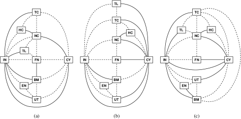
Figure 10: Planar maximally filtered graphs (PMFGs) of the ten DJUS economic sectors, constructed using half-hourly time series from (a) July 25, 2007 to August 14, 2007; (b) July 27, 2007 to August 10, 2007; and (c) July 23, 2007 to August 16, 2007. In this figure, solid links are strong links making up the MSTs, while dashed links are weaker links neglected in the MSTs.

For example, if we adopt the very simplistic criterion of having five or more links to be a center in the PMFG, we see from Fig. 11 that BM (5), CY (7), IN (7), NC (5), and TC (5) are all PMFG centers within the corresponding segment Y1, CY (9), IN (6), NC (6) are the PMFG centers within the corresponding segment G1, while BM (6), CY (5), IN (8), NC (5), HC (7) are the PMFG centers within the corresponding segment B. In particular, the PMFG structure of corresponding segment B suggests that IN and HC are the two epicenters of trading activities in October 2007. Since IN is most strongly linked to growth sectors (BM, CY, EN, FN, NC, TC) in the US economy, while HC is most strongly linked to quality sectors (TL, UT), we believe we are seeing the signatures of a ‘flight to quality’ in the early stages of the Subprime Crisis. Unlike the ‘flights to quality’ studied by economists (see for example, the recent works by Phillips and Yu, who tracked the massive flow of funds from US technology stocks to the US property market to commodities to the bond market, each time generating a bubble that crashed when the funds leave [196, 197]), the phenomenon we are seeing is within the same asset class.

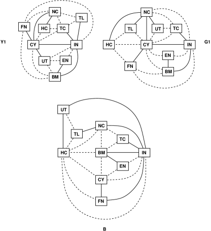
Figure 11: Planar maximally filtered graphs (PMRGs) of the corresponding segments Y1, G1, and B identified in Fig. 8. In this figure, solid links are strong links making up the MSTs, while dashed links are weaker links neglected in the MSTs.

5 MST rearrangements

Up till this point, we understood from our combined segmentation/clustering and cross-correlational analyses that the MST of the ten DJUS economic sectors presents a star-like topology during economy growth, and a chain-like topology during financial crisis (see Fig. 7). These two limiting MSTs, along with those of intermediate topologies, can also be seen at the mesoscopic scale of corresponding segments within the present financial crisis (see Fig. 9). For each corresponding segment, we then looked at the sectorial distribution of strong cross correlations, and the temporal order in which sectors made the transition, to find that strong cross correlations are frequently found at the fringe of the MST, where the volatility shocks always originate. In this section, we address the most natural question that follows: what are the natures of the correlational changes, visualized as MST rearrangements, that accompany these transitions?

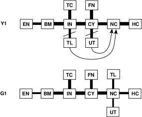
Figure 12: The MST of the corresponding segment G1 can be obtained from the MST of the corresponding segment Y1 preceding it, by breaking the TL-IN and UT-CY bonds, and forming new bonds between TL-NC and UT-NC.

5.1 Minimal MST rearrangements

If we treat the MST like a molecule, the MST rearrangements that occur from one corresponding segment to the next can be described using the chemical language of bond breaking and bond formation. This analogy is useful, because it allows us to focus on identifying the minimal set of primitive rearrangements that occur in the MST, an example of which is shown in Fig. 12. Between the successive corresponding segments Y1 and G1 identified in Fig. 8, we first note that the EN-BM-IN(-TC)-CY(-FN)-NC-HC backbone remains unchanged. We then note that TL, which is bonded to IN in Y1, and UT, which is bonded to CY in Y1, are both bonded to NC in G1. This tells us that the minimal set of primitive rearrangements necessary to get from the Y1 MST to the G1 MST consists of the breaking of the TL-IN and UT-CY bonds, and the formation of the TL-NC and UT-NC bonds. We also see from Fig. 12 that, as expected, all MST cross correlations decreased going from Y1 to G1. In fact, all cross correlations decreased going from Y1 to G1. Therefore, to have the above rearrangements, we need $C(\rm TL,NC)$ to weaken slower than $C(\rm TL,IN)$, or have $C(\rm TL,IN)$ weaken faster than $C(\rm TL,NC)$. Similarly, we need $C(\rm UT,NC)$ to weaken slower than $C(\rm UT,IN)$, or have $C(\rm UT,CY)$ weaken faster than $C(\rm UT,NC)$. In any case, we need at least one cross correlation within the (TL-IN, TL-NC) and (UT-CY, UT-NC) pairs of cross correlations to be anomalous, for the rearrangement to occur.

Figure 13: The primitive MST rearrangements going from G1 to B to Y2. The MST went from chain-like in G1 to star-like in B, to an intermediate topology in Y2.

With this ‘chemical’ understanding of minimal MST rearrangements, we now proceed to investigate the cross-correlational changes going from corresponding segments G1 to B to Y2, as shown in Fig. 13. Accompanying the Y1 to G1 transition, we saw a chain-like MST rearranging into another chain-like MST. For the G1 to B to Y2 transitions, we see the more interesting MST rearrangements from chain-like to star-like, and then to a topology intermediate between a chain and a star. As expected, more primitive rearrangements are needed to bring about the chain-to-star transition going from the moderate-volatility G1 to the low-volatility B. Ignoring the change in sector directly bonded to IN within the CY-FN pair, we see that three bonds have to be broken and reformed. These three bonds are significant, because NC is nearly a star center in the G1 MST, but loses the status after the three bonds are broken. Of course, the bonds reformed around IN, making it the star center of the B MST. A similar interaction between NC and IN occurs again for the B to Y2 transition, where NC becomes central again, with the breaking of the UT-IN and HC-UT bonds to reform around NC. Since these corresponding segments are right after the start of the Subprime Crisis, it is no wonder that NC features so prominently in the MST rearrangements.

Quantitatively, we expect cross correlations to fall generically between all sectors, when the US economy progressed from the moderate-volatility G1 segment to the low-volatility B segment. This can be seen easily from the thick bonds in the G1 MST compared to the thin bonds in the B MST in Fig. 13. In fact, the drop in average cross correlations of CY is anomalously large, from $\langle C\rangle(\rm CY)=0.80$ in G1, to $\langle C\rangle(\rm CY)=0.45$ in B. In addition, when all other cross correlations were falling, that between UT and HC increased slightly. This bucking of the trend makes the correlational changes between UT and HC highly significant statistically. Subsequently, when the US economy progressed from the low-volatility B segment to the high-volatility Y2 segment, the cross correlation between UT and HC decreased, when the cross correlations between all other sectors increased.

5.2 Early detection of economic recovery

Speaking of ‘green shoots’ of economic revival that were evident at the time, Federal Reserve chairman Ben Bernanke predicted that “America’s worst recession in decades will likely end in 2009 before a recovery gathers steam in 2010” [1]. After learning that the MST of the ten DJUS economic sectors is star-like and chain-like during the low-volatility economic growth phase and high-volatility economic crisis phase respectively, we look out for a star-like MST in the time series data of 2009 and 2010. Star-like MSTs can also be found deep inside an economic crisis phase. However, within the crisis phase, these star-like MSTs very quickly unravel to become chain-like MSTs. On the other hand, the star-shape topology is extremely robust and stable within the growth phase. Therefore, a persistent star-like MST, if it can be found, may be interpreted as the statistical signature that the US economy is firmly on track to full recovery (which may take up to two years across all sectors).

More importantly, the number of primitive rearrangements needed to transform the MST of a given period into a star-like MST indicates how close we are to the actual recovery. We can use this feature of the prerecovery MST for the early detection of economic recovery. This should be possible whether the star-like MST is a cause, in the sense that such a correlational structure within the US economy promotes growth, or an effect, in the sense that economic growth naturally results in this MST topology. Indeed, when we inspect the MST structure of the moderate-volatility G2 segment in Sep 2009, we find that it is already star-like, with IN as the star center. From Fig. 14, we see that it is two to three primitive rearrangements away from the growth MST of 2004–2005. Therefore, based on the time series data up till 25 Nov 2009, the statistical evidence summarized in the MST suggests that the US economy was already in the pre-recovery stage, and Bernanke might be prophetic to call for an actual economic recovery in 2010.

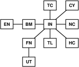
(a)

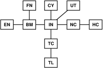
(b)

Figure 14: Comparison of the MSTs for (a) the 2004–2005 growth period, and (b) the moderate-volatility segment around September 2009.

5.3 Comparison between previous and present recoveries

Since the time series data we have covers the recovery periods for both financial crises, we wanted also to compare the sequence of pre-recovery MSTs for the previous crisis against the ones we see for the present crisis. We immediately encountered two problems. First, volatility movements in the various sectors between 2002 and 2004 are much less coordinated than those we find in the present financial crisis, and thus it is difficult to find corresponding segments. Second, for successive corresponding segments that we can find for the 2002–2004, successive MSTs are structurally very different from each other, suggesting very violent rearrangements within the MSTs. In Fig. 15, we show the MSTs of four successive corresponding segments identified before and after the 11 Sep 2001 attack, from August 2001 to December 2001. These corresponding segments, an August 2001 moderate-volatility segment before the 11 Sep 2001 attack, a two-week extremely-high-volatility segment right after the attack, a October 2001 high-volatility segment following this, and a November–December 2001 moderate-volatility segment afterwards, are amongst the most well-defined ones that we can identified through the previous financial crisis. As we can see, it is impossible to assign a small number of bonds that must be broken and reformed to go from one MST to the next. Throughout the violent rearrangements, IN remained at the center of the MSTs. We also see that the MST is chain-like before and after the 11 Sep 2001 attack, became briefly star-like in the October 2001 high-volatility segment, before unravelling again to a chain-like MST for the rest of the year.

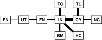
(a)

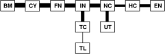
(b)

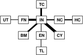
(c)

(d)

Figure 15: MSTs for successive corresponding segments: (a) moderate-volatility segment before the 11 Sep 2001 attack on the World Trade Center; (b) extremely-high-volatility segment right after the 11 Sep 2001 attack; (c) high-volatility segment following; and (d) moderate-volatility segment following.

6 Conclusions

To summarize, we performed a cross-section analysis on the high-frequency time series of the ten DJUS economic sector indices between February 2000 and November 2009, to discover statistical signatures that can be used to forecast economic recovery. The half-hourly time series of these indices are first segmented individually using a recursive entropic segmentation scheme. The segments of each economic sector are then hierarchically clustered into between four and seven clusters, representing the growth, crisis, correction, and crash macroeconomic phases. In our previous study [27], we compared the temporal distributions of clustered segments across all ten economic sectors, to see that the US economy emerged from the previous technology bubble financial crisis starting mid-2003, enjoyed a four-year period of growth, and then succumbed to the present property bubble financial crisis starting mid-2007. From this cross-section of temporal distributions of clustered segments, we also see the US economy taking one and a half years to completely recover from the previous financial crisis, but only two months to completely enter the present financial crisis. More interestingly, for the present financial crisis, we find the volatility dynamics within the US economic sectors to be strongly driven by interest rate cuts by the Federal Reserve. Of the seven interest rate cuts made over 2007 and 2008, the first two lowered market volatilities, the next two raised market volatilities, while the last three had no permanent effect on market volatilities.

In this paper, we extended the cross-section analysis, by constructing the cross-correlation matrices and therefrom the MSTs of the ten DJUS economic sectors first over February 2000 to August 2008, and the two-year intervals 2002–2003, 2004–2005, 2008–2009, as well as the 11 corresponding segments identified in Fig. 8. In general, we find stronger cross correlatons when the market volatility is high, and weaker cross correlations when the market volatility is low. We also find evidence that cross correlations within the US economy have been increasing over the years. In all MSTs, we find a core-fringe structure, with CY, IN, and NC forming the core, and HC, TL, UT residing on the fringe. In spite of the supposed market turmoil we expect throughout the present financial crisis, a highly conserved EN-BM-IN-CY-NC-TC-HC backbone can be identified in most of the MSTs. Through an enhanced visualization scheme for the MSTs, we see a dynamic core of strongly-correlated sectors, which expands and contracts in tandem with changes in the overall market volatility. In addition, for all 11 corresponding segments studied, we find the volatility shocks starting always at the fringe, frequently accompanied by anomalously high cross correlations here, and propagating inwards towards the core of the MST. These volatility shocks originate mostly from the US domestic fringe sectors, which are weakly coupled to the world market, instead of coming from EN and BM, which are most strongly coupled to the global supply and demand cycles.

More importantly, we see that the MSTs of the ten DJUS economic sectors can be classified into two distinct topologies: star-like and chain-like. The MST is robustly star-like during economic growth, with IN at the center, and robustly chain-like within an economic crisis. For the present financial crisis, the MST of a corresponding segment can be obtained from the MST of the preceding corresponding segment through a small set of primitive rearrangements. In contrast, very violent rearrangements are implied going from the MST of one corresponding segment to the MST of the next corresponding segment within the previous, mid-1998 to mid-2003, financial crisis. This suggests that the US economy has become more efficient in processing information arising from volatility shocks. Combining these two observations, we postulated that the star-like MST seen in the Sep 2009 G2 corresponding segment indicates that the US economy was in the early stages of economic recovery.

After this study was completed, US market volatilities remained moderate to high until the start of May 2010, when investor confidence was again tested, first by the glitch in the NYSE electronic trading platform, and then by the unfolding Greek Debt Crisis. Market volatilities skyrocketed, and even after the European Union announced their bailout plan for Greece, the atmosphere of economic uncertainty lingered. When interviewed in July 2010 on NBC’s “Meet the Press” programme, US Treasury Secretary Timothy Geithner acknowledged the slow recovery of the US economy, but added that it is gradually gaining strength [198]. A commentary that appears the same day Geithner’s interview was aired complicates the mood, by citing economists who warn that recent gains in the stock market need not be an indicator of economic recovery [199]. In fact, on 24 Aug 2010, world stock markets fell over concerns that the yen is too strong for the good of the Japanese economy, and also over more bad news anticipated from the US economic reports due to be released the same week [200].

Figure 16: MSTs for four successive corresponding segments straddling the Greek debt crisis: Gr1 (extremely high volatility, 21 Jan to 15 Feb 2010), Gr2 (moderate to high volatility, 1–31 Mar 2010), and Gr3 (extremely high volatility, 1 May to 15 Jul 2010).

To check if the US economic recovery might have been derailed by the Greek Debt Crisis, we segmented the DJUS economic sector time series from January to July 2010, and constructed MSTs for three corresponding segments. The MSTs for these three corresponding segments, the extremely-high-volatility Gr1 segment (21 Jan–15 Feb 2010) and moderate-volatility Gr2 segment (1–31 Mar 2010) before the Greek Debt Crisis, and the extremely-high-volatility Greek Debt Crisis Gr3 segment itself (1 May–15 Jul 2010), are shown in Fig. 16. As we can see, even though market volatilities are high, the MST presented a very robust star shape in all three corresponding segments. While they are nervous, it appears that investor sentiments during the Greek Debt Crisis are distinctly different from those seen over 2008 and the first half of 2009. Judging from the increasingly star-like MST, it appears that the US economy is staying its course to the long-awaited economic recovery.

Appendix A Top components of Dow Jones US economic sector indices

A.1 Basic Materials

ISIN/Ticker	Company	Adjusted Weight
FCX	Freeport-McMoRan Copper & Gold Inc.	10.29%
DD	E.I. DuPont de Nemours & Co.	9.12%
DOW	Dow Chemical Co.	7.70%
NEM	Newmont Mining Corp.	6.14%
PX	Praxair Inc.	6.13%
APD	Air Products & Chemicals Inc.	3.67%
BTU	Peabody Energy Corp.	3.38%
AA	Alcoa Inc.	2.89%
PPG	PPG Industries Inc.	2.78%
ECL	Ecolab Inc.	2.41%

A.2 Consumer Services

ISIN/Ticker	Company	Adjusted Weight
WMT	Wal-Mart Stores Inc.	7.28%
MCD	McDonald’s Corp.	5.33%
DIS	Walt Disney Co.	4.15%
AMZN	Amazon.com Inc.	3.90%
HD	Home Depot Inc.	3.28%
CVS	CVS Caremark Corp.	2.70%
CMCSA	Comcast Corp. Cl A	2.64%
TGT	Target Corp.	2.44%
DTV	DIRECTV Group Inc.	2.30%
WAG	Walgreen Co.	2.18%

A.3 Oil & Gas

ISIN/Ticker	Company	Adjusted Weight
XOM	Exxon Mobil Corp.	25.57%
CVX	Chevron Corp.	11.68%
SLB	Schlumberger Ltd.	7.59%
COP	ConocoPhillips	6.01%
OXY	Occidental Petroleum Corp.	5.14%
APA	Apache Corp.	2.96%
HAL	Halliburton Co.	2.47%
APC	Anadarko Petroleum Corp.	2.28%
DVN	Devon Energy Corp.	2.08%
NOV	National Oilwell Varco Inc.	1.84%

A.4 Financials

ISIN/Ticker	Company	Adjusted Weight
JPM	JPMorgan Chase & Co.	7.50%
WFC	Wells Fargo & Co.	6.73%
BAC	Bank of America Corp.	5.50%
C	Citigroup Inc.	5.04%
GS	Goldman Sachs Group Inc.	3.40%
BRK/B	Berkshire Hathaway Inc. Cl B	3.38%
AXP	American Express Co.	2.32%
USB	U.S. Bancorp	2.30%
V	VISA Inc. Cl A	1.85%
BK	Bank of New York Mellon Corp.	1.65%

A.5 Healthcare

ISIN/Ticker	Company	Adjusted Weight
JNJ	Johnson & Johnson	12.56%
PFE	Pfizer Inc.	9.68%
MRK	Merck & Co. Inc.	7.82%
ABT	Abbott Laboratories	5.28%
AMGN	Amgen Inc.	3.72%
BMY	Bristol-Myers Squibb Co.	3.20%
UNH	UnitedHealth Group Inc.	3.03%
MDT	Medtronic Inc.	2.68%
LLY	Eli Lilly & Co.	2.44%
GILD	Gilead Sciences Inc.	2.26%

A.6 Industrials

ISIN/Ticker	Company	Adjusted Weight
GE	General Electric Co.	10.45%
UTX	United Technologies Corp.	4.03%
MMM	3M Co.	3.39%
UPS	United Parcel Service Inc. Cl B	3.10%
CAT	Caterpillar Inc.	2.98%
UNP	Union Pacific Corp.	2.77%
BA	Boeing Co.	2.58%
EMR	Emerson Electric Co.	2.57%
HON	Honeywell International Inc.	2.15%
DE	Deere & Co.	1.95%

A.7 Consumer Goods

ISIN/Ticker	Company	Adjusted Weight
PG	Procter & Gamble Co.	13.34%
KO	Coca-Cola Co.	10.35%
PM	Philip Morris International Inc.	8.02%
PEP	PepsiCo Inc.	7.91%
F	Ford Motor Co.	4.09%
MO	Altria Group Inc.	3.85%
KFT	Kraft Foods Inc. Cl A	3.73%
CL	Colgate-Palmolive Co.	2.90%
MON	Monsanto Co.	2.50%
NKE	Nike Inc. Cl B	1.97%

A.8 Technology

ISIN/Ticker	Company	Adjusted Weight
AAPL	Apple Inc.	13.57%
MSFT	Microsoft Corp.	9.33%
IBM	International Business Machines Corp.	8.58%
GOOG	Google Inc. Cl A	6.52%
INTC	Intel Corp.	5.65%
CSCO	Cisco Systems Inc.	5.31%
ORCL	Oracle Corp.	4.98%
HPQ	Hewlett-Packard Co.	4.73%
QCOM	Qualcomm Inc.	3.61%
EMC	EMC Corp.	2.11%

A.9 Telecommunications

ISIN/Ticker	Company	Adjusted Weight
T	AT&T Inc.	44.32%
VZ	Verizon Communications Inc.	24.29%
AMT	American Tower Corp. Cl A	5.45%
CTL	CenturyLink Inc.	3.47%
S	Sprint Nextel Corp.	2.99%
CCI	Crown Castle International Corp.	2.75%
Q	Qwest Communications International Inc.	2.67%
FTR	Frontier Communications Corp.	2.44%
VMED	Virgin Media Inc.	2.03%
NIHD	NII Holdings Inc.	1.72%

A.10 Utilities

ISIN/Ticker	Company	Adjusted Weight
SO	Southern Co.	6.68%
EXC	Exelon Corp.	5.61%
D	Dominion Resources Inc. (Virginia)	5.28%
DUK	Duke Energy Corp.	4.94%
NEE	NextEra Energy Inc.	4.52%
PCG	PG&E Corp.	3.96%
AEP	American Electric Power Co. Inc.	3.67%
PEG	Public Service Enterprise Group Inc.	3.38%
SE	Spectra Energy Corp.	3.32%
ED	Consolidated Edison Inc.	2.93%

References

- [1] Reuters News, “Bernanke sees U.S. recovery beginning in 2010”, 16 Mar 2009. URL: http://www.reuters.com/article/idUSTRE52E22520090316.
- [2] FRB: Open Market Operations, Board of Governors of the Federal Reserve System. URL: http://www.federalreserve.gov/monetarypolicy/openmarket.htm.
- [3] Reuters News, “Increasingly hawkish Fed ponders raising rates”, 3 Jun 2010. URL: http://www.reuters.com/article/idUSTRE65263920100603.
- [4] D. C. Rose and L. H. White, “Ease up on the gas pedal, Bernanke!”, The Cato Institute, 10 Mar 2009. URL: http://www.cato.org/pub_display.php?pub_id=10033.
- [5] S. H. Hanke, “Fed up”, The Cato Institute, 24 Apr 2009. URL: http://www.cato.org/pub_display.php?pub_id=10146.
- [6] A. Xie, “China swallows Obama’s stimulus for the US”, Comments & Analysis, Today, p. 22, 19 Aug 2010.
- [7] D. T. Armentano, “Memo to Federal Reserve: Increase interest rates now!”, The Cato Institute, 13 Jan 2004. URL: http://www.cato.org/pub_display.php?pub_id=2510.
- [8] M. Chauvet, “Stock market fluctuations and the business cycle ”, Journal of Economic and Social Measurement, vol. 25, no. 3–4, pp. 235–257, 1998.
- [9] M. Camacho, “Vector smooth transition regression models for US GDP and the composite index of leading indicators”, Journal of Forecasting, vol. 23, no. 3, pp. 173–196, 2004.
- [10] M. Marcellino, “Leading indicators”, in Handbook of Economic Forecasting, vol. 1, edited by G. Elliott, C. W. J. Granger, and A. Timmermann, Chapter 16, pp. 879–960, Elsevier (2006).
- [11] P. Kannan, P. Rabanal, and A. Scott, “Macroeconomic patterns and monetary policy in the run-up to asset price busts”, IMF Working Paper 09/252, Nov 2009.
- [12] G. Chalamandaris and A. E. Tsekrekos, “The correlation structure of FX option markets before and since the financial crisis”, Applied Financial Economics, vol. 20, no. 1, pp. 73–84, 2010.
- [13] J. L. Simpson, “Were there warning signals from banking sectors for the 2008/2009 global financial crisis?”, Applied Financial Economics, vol. 20, no. 1, pp. 45–61, 2010.
- [14] N. Tamirisa, “Forecasting recessions: consensus and disagreement”, IMF Research Bulletin, vol. 11, no. 1, pp. 1–3, 2010.
- [15] M. D. Bordo and J. G. Haubrich, “Credit crises, money and contractions: An historical view”, Journal of Monetary Economics, vol. 57, no. 1, pp. 1–18, 2009.
- [16] J. Boyd, G. de Nicolò, and E. Loukoianova, “Banking crises and crisis dating: theory and evidence”, IMF Working Paper 09/141, Jul 2009.
- [17] S. Claessens, M. A. Kose, and M. E. Terrones, “What happens during recessions, crunches, and busts?”, Economic Policy, vol. 24, no. 60, pp. 653–700, 2009.
- [18] S. G. Cecchetti, M. Kohler, and C. Upper, “Financial crises and economic activity”, NBER Working Paper 15379, Sep 2009. URL: http://www.nber.org/papers/w15379.
- [19] J. Boysen-Hogrefe, N. Jannsen, and C.-P. Meier, “The ugly and the bad: banking and housing crises strangle output permanently, ordinary recessions do not”, Kiel Institute for the World Economy Working Paper 1586, Jan 2010.
- [20] S. Claessens, M. A. Kose, and M. E. Terrones, “The global financial crisis: how similar? how different? how costly?”, Journal of Asian Economics, vol. 21, no. 3, pp. 247–264, 2010.
- [21] M. Chauvet and S. Potter, “Coincident and leading indicators of the stock market”, Journal of Empirical Finance, vol. 7. no. 1, pp. 87–111, 2000.
- [22] M. Biggs, T. Mayer, and A. Pick, “Credit and economic recovery”, DNB Working Paper 218, Jul 2009.
- [23] A. Mirestean and C. Tsangarides, “Searching for robust growth determinants”, IMF Research Bulletin, vol. 11, no. 1, pp. 1, 4–5, 2010.
- [24] P. Bernaola-Galván, R. Román-Roldán, and J. L. Oliver, “Compositional Segmentation and Long-Range Fractal Correlations in DNA Sequences”, Physical Review E, vol. 53, no. 5, pp. 5181–5189, 1996.
- [25] R. Román-Roldán, P. Bernaola-Galván, and J. L. Oliver, “Sequence Compositional Complexity of DNA through an Entropic Segmentation Method”, Physical Review Letters, vol. 80, no. 6, pp. 1344–1347, 1998.
- [26] J. C. Wong, H. Lian, and S. A. Cheong, “Detecting macroeconomic phases in the Dow Jones Industrial Average time series”, Physica A, vol. 388, no. 21, pp. 4635–4645, 2009.
- [27] G. H. T. Lee, Y. Zhang, J. C. Wong, M. Prusty, and S. A. Cheong, “Causal links in US economic sectors”, arXiv:0911.4763, 25 Nov 2009.
- [28] W. Yan, R. Woodard, and D. Sornette, “Diagnosis and prediction of tipping points in financial markets: crashes and rebounds”, arXiv:1001.0265, 6 Feb 2010.
- [29] A. Mamun, M. K. Hassan, and M. Johnson, “How did the Fed do? An empirical assessment of the Fed’s new initiatives in the financial crisis”, Applied Financial Economics, vol. 20, no. 1, pp. 15–30, 2010.
- [30] D. Dittman and R. S. Conrad, “Second derivatives, green shoots and …caution”, Investing Daily, 5 May 2009. URL: http://www.investingdaily.com/ce/15411/second-derivatives-green-shoots-andcaution.html.
- [31] Telegraph.co.uk, “Stephen Hester: I don’t see any green shoots”, 8 May 2009. URL: http://www.telegraph.co.uk/finance/newsbysector/banksandfinance/5296905/Stephen-Hester-I-dont-see-any-green-shoots.html.
- [32] Bloomberg News, “Trichet Says Global Economy Is Near Turning Point (Update1)”, 11 May 2009. URL: http://www.bloomberg.com/apps/news?pid=20601087&sid=azaqSX6AfB0g&refer=home.
- [33] N. Roubini, “Green Shoots Or Yellow Weeds?”, commentary in Forbes, 14 May 2009. URL: http://www.forbes.com/2009/05/13/recession-global-economy-china-green-shoots-opinions-columnists-nouriel-roubini.html.
- [34] Channel News Asia, “Market watchers express less optimism over green shoots theory”, 2 Jul 2009. URL: http://www.channelnewsasia.com/stories/singaporebusinessnews/view/440027/1/.html.
- [35] P. du Plessis, “Caution remains over the robustness of any economic recovery”, The Market Oracle, 30 Aug 2009. URL: http://www.marketoracle.co.uk/Article13095.html.
- [36] Bloomberg News, “China Needs ‘Very Certain’ Recovery for Stimulus End, Zhou Says”, 24 March 2010. URL: http://www.bloomberg.com/apps/news?pid=20601068&sid=aK2stfFGYL2o.
- [37] CNNMoney.com, “Fed: Recovery may lose steam”, 6 Apr 2010. URL: http://money.cnn.com/2010/04/06/news/economy/Fed_meeting_minutes/index.htm?cnn=yes&hpt=Sbin.
- [38] Formerly Taqtic, SIRCA, https://taqtic.sirca.org.au/TaqTic/. Now available as Thomson Reuters Datascope Tick History, https://tickhistory.datascope.reuters.com/.
- [39] S. J. Taylor and X. Xu, “The Incremental Volatility Information in One Million Foreign Exchange Quotations”, Journal of Empirical Finance, vol. 4, no. 4, pp. 317–340, 1997.
- [40] M. M. Dacorogna, U. A. Müller, R. B. Olsen, and O. V. Pictet, “Modelling Short-term Volatility with GARCH and HARCH Models”, in Nonlinear Modelling of High Frequency Financial Time Series edited by C. Dunis and B. Zhou, pp. 161–176, John Wiley (Chichester, 1998).
- [41] G. W. Schwert, “Stock Market Volatility: Ten Years After the Crash”, in Brookings-Wharton Papers on Financial Services edited by R. E. Litan and A. M. Santomero, pp. 65–99, The Brookings Institution (Washington DC, USA, 1998).
- [42] T. G. Andersen, T. Bollerslev, F. X. Diebold, and P. Labys, “The distribution of realized exchange rate volatility”, Journal of the American Statistical Association, vol. 96, no. 453, pp. 42–55, 2001.
- [43] T. G. Andersen, T. Bollerslev, F. X. Diebold, and H. Ebens, “The distribution of realized stock return volatility”, Journal of Financial Economics, vol. 61, no. 1, pp. 43–76, 2001.
- [44] T. Conlon, H. J. Ruskin, and M. Crane, “Multiscaled cross-correlation dynamics in financial time series”, arXiv:1001.0497, 4 Jan 2010.
- [45] J.-J. Tseng and S.-P. Li, “Asset returns and volatility clustering in financial time series”, arXiv:1002.0284, 1 Feb 2010.
- [46] A. D. Spetiotopoulos, “Volatilities that change with time: the temporal behavior of the distribution of stock-market prices”, arXiv:1007.5274, 29 Jul 2010.
- [47] S. M. Goldfeld and R. E. Quandt, “A Markov model for switching regressions”, Journal of Econometrics, vol. 1, pp. 3–16, 1973.
- [48] J. D. Hamilton, “A new approach to the economic analysis of nonstationary time series and the business cycle”, Econometrica, vol. 57, pp. 357–384, 1989.
- [49] C.-J. Kim and C. R. Nelson, “Has the U.S. economy become more stable? A Bayesian approach based on a Markov-switching model of business cycle”, Review of Economics and Statistics, vol. 81, pp. 608–616, 1999.
- [50] J. Bai, “Least squares estimation of a shift in linear processes”, Journal of Time Series Analysis, vol. 15, no. 5, pp. 453–472, 1994.
- [51] J. Bai, “Least absolute deviation estimation of a shift”, Econometric Theory, vol. 11, no. 3, pp. 403–436, 1995.
- [52] T. T.-L. Chong, “Partial parameter consistency in a misspecified structural change model”, Economics Letters, vol. 49, no. 4, pp. 351–357, 1995.
- [53] C. R. Loader, “Change point estimation using nonparametric regression”, Annals of Statistics, vol. 24, no. 4, pp. 1667–1678, 1996.
- [54] J. Bai, “Estimation of a change point in multiple regression models”, The Review of Economics and Statistics, vol. 79, no. 4, pp. 551–563, 1997.
- [55] R. L. Lumsdaine and D. H. Papell, “Multiple Trend Breaks and the Unit-Root Hypothesis”, Review of Economics and Statistics, vol. 79, no. 2, pp. 212–218, 1997.
- [56] J. Bai and P. Perron, “Estimating and Testing Linear Models with Multiple Structural Changes”, Econometrica, vol. 66, no. 1, pp. 47–78, 1998.
- [57] M. Lavielle and E. Moulines, “Least-squares estimation of an unknown number of shifts in a time series”, Journal of Time Series Analysis, vol. 21, no. 1, pp. 33–59, 2000.
- [58] T. T.-L. Chong, “Structural change in AR(1) models”, Econometric Theory, vol. 17, no. 1, pp. 87–155, 2001.
- [59] B. E. Hansen, “The new econometrics of structural change: dating breaks in U.S. labor productivity”, The Journal of Economic Perspectives, vol. 15, no. 4, pp. 117–128, 2001.
- [60] E. Zivot and D. W. K. Andrews, “Further evidence on the Great Crash, the oil-price shock, and the unit-root hypothesis”, Journal of Business and Economic Statistics, vol. 20, no. 1, pp. 25–44, 2002.
- [61] J. Bai and P. Perron, “Computation and analysis of multiple structural change models”, Journal of Applied Econometrics, vol. 18, no. 1, pp. 1–21, 2003.
- [62] P. Perron and X. Zhu, “Structural breaks with deterministic and stochastic trends”, Journal of Econometrics, vol. 129, no. 1–2, pp. 65–119, 2005.
- [63] W. Guo and M. E. Wohar, “Identifying regime changes in market volatility”, Journal of Financial Research, vol. 29, no. 1, pp. 79–93, 2006.
- [64] J. L. Carrion-i-Silvestre, D. Kim, and P. Perron, “GLS-based unit root tests with multiple structural breaks under both the null and the alternative hypotheses”, Econometric Theory, vol. 25, no. 6, pp. 1754–1792, 2009.
- [65] G. Vaglica, F. Lillo, E. Moro, and R. N. Mantegna, “Scaling laws of strategic behavior and size heterogeneity in agent dynamics”, Physical Review E, vol. 77, no. 3, 036110, 2008.
- [66] B. Tóth, F. Lillo, and J. D. Farmer, “Segmentation algorithm for non-stationary compound Poisson processes”, arXiv:1001.2549, 14 Jan 2010.
- [67] R. N. Mantegna and H. E. Stanley, “Scaling Behaviour in the Dynamics of an Economic Index”, Nature, vol. 376, pp. 46–49, 1995.
- [68] L. Kullmann, J. Töyli, J. Kertesz, A. Kanto, and K. Kaski, “Characteristic times in stock market indices”, Physica A, vol. 269, no. 1, pp. 98–110, 1999.
- [69] E. Fama and R. Roll, “Parameter estimates for symmetric stable distributions”, Journal of the American Statistical Association, vol. 66, no. 334, pp. 331–338, 1971.
- [70] B. M. Hill, “A simple general approach to inference about the tail of a distribution”, The Annals of Statistics, vol. 3, no. 5, pp. 1163–1174, 1975.
- [71] I. A. Koutrouvelis, “Regression-type estimation of the parameters of stable laws”, Journal of the American Statistical Association, vol. 75, no. 372, pp. 918–928, 1980.
- [72] I. A. Koutrouvelis, “An iterative procedure for the estimation of the parameters of stable laws”, Communications in Statistics — Simulation and Computation, vol. 10, no. 1, pp. 17–28, 1981.
- [73] J. H. McCulloch, “Simple consistent estimators of stable distribution parameters”, Communications in Statistics — Simulation and Computation, vol. 15, no. 4, pp. 1109–1136, 1986.
- [74] V. M. Zolotarev, One-Dimensional Stable Distributions, American Mathematical Society, 1986.
- [75] J. P. Nolan, “Parameterizations and modes of stable distributions”, Statistics & Probability Letters, vol. 38, no. 2, pp. 187–195, 1998.
- [76] J. P. Nolan, “Maximum likelihood estimation and diagnostics for stable distributions”, in Lévy Processes edited by O. E. Barndorff-Nielsen, T. Mikosch, and S. I. Resnick, pp. 379–400, Birkhäuser, 2001.
- [77] G. J. Worsdale, “Tables of cumulative distribution functions for symmetric stable distributions”, Journal of the Royal Statistical Society Series C (Applied Statistics), vol. 24, no. 1, pp. 123–131, 1975.
- [78] D. B. Panton, “Cumulative distribution function values for symmetric standardized stable distributions”, Communications in Statistics — Simulation and Computation, vol. 21, no. 2, pp. 485–492, 1992.
- [79] J. H. McCulloch and D. B. Panton, “Precise tabulation of the maximally-skewed stable distributions and densities”, Computational Statistics & Data Analysis, vol. 23, no. 3, pp. 307–320, 1997.
- [80] J. P. Nolan, “Numerical calculation of stable densities and distribution functions”, Stochastic Models, vol. 13, no. 4, pp. 759–774, 1997.
- [81] J. P. Nolan, “An algorithm for evaluating stable densities in Zolotarev’s () parameterization”, Mathematical and Computer Modelling, vol. 29, no. 10–12, pp. 229–233, 1999.
- [82] L. C. F. Eng, Financial Time Series Segmentation Based on Lévy Stable Distributions, B.Sc. (Mathematical Sciences) final year project report, Nanyang Technological University, Apr 2010.
- [83] J. Lin, “Divergence measures based on the Shannon entropy”, IEEE Transactions on Information Theory, vol. 37, no. 1, pp. 145–151, 1991.
- [84] S.-A. Cheong, P. Stodghill, D. J. Schneider, S. W. Cartinhour, and C. R. Myers, “Extending the Recursive Jensen-Shannon Segmentation of Biological Sequences”, q-bio/0904.2466.
- [85] W. Li, “New Stopping Criteria for Segmenting DNA Sequences”, Physical Review Letters, vol. 86, no. 25, pp. 5815–5818, 2001.
- [86] W. Li, “DNA Segmentation as a Model Selection Process”, Proceedings of the International Conference on Research in Computational Molecular Biology (RECOMB), pp. 204–210, 2001.
- [87] S.-A. Cheong, P. Stodghill, D. J. Schneider, S. W. Cartinhour, and C. R. Myers, “The Context Sensitivity Problem in Biological Sequence Segmentation”, q-bio/0904.2668.
- [88] R. K. Azad, J. S. Rao, W. Li, and R. Ramaswamy, “Simplifying the mosaic description of DNA sequences”, Physical Review E, vol. 66, no. 3, 031913, 2002.
- [89] A. Jain, M. Murty, and P. Flynn, “Data Clustering: A Review”, ACM Computing Surveys, vol. 31, no. 3, pp. 264–323, 1999.
- [90] F. B. Baker, “Numerical taxonomy for educational researchers”, Review of Educational Research, vol. 42, no. 3, pp. 345–358, 1972.
- [91] P. H. A. Sneath, “The application of computers to taxonomy”, Journal of General Microbiology, vol. 17, pp. 201–226, 1957.
- [92] S. C. Johnson, “Hierarchical clustering schemes”, Psychometrika, vol. 32, no. 3, pp. 241–254, 1967.
- [93] F. B. Baker, “Stability of two hierarchical grouping techniques case 1: sensitivity to data errors”, Journal of the American Statistical Association, vol. 69, no. 346, pp. 440–445, 1974.
- [94] J. J. van Wijk and E. R. van Selow, “Cluster and Calendar Based Visualization of Time Series Data”, Proceedings of the 1999 IEEE Symposium on Information Visualization (Oct 24–29, 1999, San Francisco, California, USA), pp. 4–9, 1999.
- [95] A. Krawiecki, J. A. Hołyst, and D. Helbing, “Volatility Clustering and Scaling for Financial Time Series due to Attractor Bubbling”, Physical Review Letters, vol. 89, no. 15, 158701, 2002.
- [96] T. C. Fu, F. L. Chung, R. Luk, and C.-M. Ng, “Financial Time Series Indexing Based on Low Resolution Clustering”, Proceedings of the ICDM 2004 Workshop on Temporal Data Mining: Algorithms, Theory and Applications (Nov 1–4, 2004, Brighton, UK), pp. 4–13, 2004.
- [97] D. B. Panton, V. P. Lessig, and O. M. Joy, “Comovement of international equity markets: a taxonomic approach”, Journal of Financial and Quantitative Analysis, vol. 11, no. 3, pp. 415–432, 1976.
- [98] A. C. Stockman and L. L. Tesar, “Tastes and technology in a two-country model of the business cycle: explaining international comovement”, The American Economic Review, vol. 85, no. 1, pp. 168–185, 1995.
- [99] G. A. Karolyi and R. M. Stulz, “Why Do Markets Move Together? An Investigation of U.S.-Japan Stock Return Comovements”, Journal of Finance, vol. 51, no. 3, pp. 951–986, 1996.
- [100] C. Croux, M. Forni, and L. Reichlin, “A measure of comovement for economic variables: theory and empirics”, Review of Economics and Statistics, vol. 83, no. 2, pp. 232–241, 2001.
- [101] K. J. Forbes and R. Rigobon, “No contagion, only interdependence: measuring stock market comovements”, Journal of Finance, vol. 57, no. 5, pp. 2223–2261, 2002.
- [102] N. Barberis, A. Shleifer, and J. Wurgler, “Comovement”, Journal of Financial Economics, vol. 75, no. 2, pp. 283–317, 2005.
- [103] M. Baxter and M. A. Kouparitsas, “Determinants of business cycle comovement: a robust analysis”, Journal of Monetary Economics, vol. 52, no. 1, pp. 113–157, 2005.
- [104] O. E. Barndorff-Nielsen and N. Shepard, “Econometrics of Testing for Jumps in Financial Economics Using Bipower Variation”, Journal of Financial Econometrics, vol. 4, no. 1, pp. 1–30, 2006.
- [105] T. Bollerslev, T. H. Law, and G. Tauchen, “Risk, jumps, and diversification”, Journal of Econometrics, vol. 144, no. 1, pp. 234–256, 2008.
- [106] J. Jacod and V. Todorov, “Testing for common arrivals of jumps for discretely observed multidimensional processes”, Annals of Statistics, vol. 37, no. 4, pp. 1792–1838, 2009.
- [107] F. Canova and J. Marrinan, “Sources and propagation of international output cycles: Common shocks or transmission?”, Journal of International Economics, vol. 46, no. 1, pp. 133–166, 1998.
- [108] R. Rigobon, “On the measurement of the international propagation of shocks: is the transmission stable?”, Journal of International Economics, vol. 61, no. 2, pp. 261–283, 2003.
- [109] D. W. K. Andrews, “Cross-section regression with common shocks”, Econometrica, vol. 73, no. 5, pp. 1551–1585, 2005.
- [110] J. Bai, R. L. Lumsdaine, and J. H. Stock, “Testing for and dating common breaks in multivariate time series”, Review of Economic Studies, vol. 65, no. 3, pp. 395–432, 1998.
- [111] J. L. Carrion-i-Silvestre, T. Del Barrio-Castro, and E. López-Bazo, “Breaking the panels: An application to the GDP per capita”, Econometrics Journal, vol. 8, no. 2, pp. 159–175, 2005.
- [112] K.-S. Im, J. Lee, and M. Tieslau, “Panel LM unit-root tests with level shifts”, Oxford Bulletin of Economics and Statistics, vol. 67, no. 3, pp. 393–419, 2005.
- [113] J. Bai, “Panel data models with interactive fixed effects”, Econometrica, vol. 77, no. 4, pp. 1229–1279, 2009.
- [114] J. Bai and J. L. Carrion-i-Silvestre, “Structural changes, common stochastic trends, and unit roots in panel data”, Review of Economic Studies, vol. 76, no. 2, pp. 471–501, 2009.
- [115] D. Kim, “Estimating a common deterministic time trend break in large panels with cross sectional dependence”, working paper, 17 Oct 2009.
- [116] Investopedia, “What does a cut in interest rates mean for the stock market?”, http://www.investopedia.com/ask/answers/132.asp.
- [117] N. Frank, B. González-Hermosillo, and H. Hesse, “Transmission of liquidity shocks: Evidence from the 2007 Subprime Crisis”, IMF Working Paper WP/08/200, August 2008. Available from http://www.banquefrance.eu/fr/publications/telechar/seminaires/2008/Hermosillo-gonzales.pdf.
- [118] A. W. Lo, “Hedge funds, systemic risk, and the financial crisis of 2007–2008”, written testimony prepared for the US House of Representatives Committee on Oversight and Government Reform, 13 November 2008. Revised version published as A. W. Lo, “Regulatory reform in the wake of the financial crisis of 2007–2008”, Journal of Financial Economic Policy, vol. 1, no. 1, pp. 4–43, 2009.
- [119] C. Tudor, “Understanding the roots of the US Subprime Crisis and its subsequent effects”, The Romanian Economic Journal, no. 31, pp. 115–148, 2009.
- [120] W. Cheung, S. Fung, and S.-C. Tsai, “Global capital market interdependence and spillover effect of credit risk: evidence from the 2007-2009 global financial crisis”, Applied Financial Economics, vol. 20, no. 1, pp. 85–103, 2010.
- [121] M. C. Münnix, R. Schäfer, and O. Grothe, “Estimating correlation and covariance matrices by weighting of market similarity”, arXiv:1006.5847, 30 Jun 2010.
- [122] D. K. T. Wong and K.-W. Li, “Comparing the performance of relative stock return differential and real exchange rate in two financial crises”, Applied Financial Economics, vol. 20, no. 1, pp. 137–150, 2010.
- [123] L. Laloux, P. Cizeau, J.-P. Bouchaud, and M. Potters, “Noise dressing of financial correlation matrices”, Physical Review Letters, vol. 83, no. 7, pp. 1467–1470, 1999.
- [124] V. Plerou, P. Gopikrishnan, B. Rosenow, L. A. N. Amaral, T. Guhr, and H. E. Stanley, “Random matrix approach to cross correlations in financial data”, Physical Review E, vol. 65, no. 6, 066126, 2002.
- [125] A. Utsugi, K. Ino, M. Oshikawa, “Random matrix theory analysis of cross correlations in financial markets”, Physical Review E, vol. 70, no. 2, 026110, 2004.
- [126] D. Wilcox and T. Gebbie, “On the analysis of cross-correlations in South African market data”, Physica A, vol. 344, pp. 294–298, 2004.
- [127] D. Wilcox and T. Gebbie, “An analysis of cross-correlations in an emerging market”, Physica A, vol. 375, pp. 584–598, 2007.
- [128] S. Çukur, M. Eryiğit, and R. Eryiğit, “Cross correlations in an emerging market financial data”, Physica A, vol. 376, pp. 555–564, 2007.
- [129] V. Kulkarni and N. Deo, “Correlation and volatility in an Indian stock market: A random matrix approach”, The European Physical Journal B, vol. 60, pp. 101–109, 2007.
- [130] J. Shen and B. Zheng, “Cross-correlation in financial dynamics”, Europhysics Letters, vol. 86, 48005, 2009.
- [131] M. Girvan and M. E. J. Newman, “Community structure in social and biological networks”, Proceedings of the National Academy of Sciences of the United States of America, vol. 99, no. 12, pp. 7821–7826, 2002.
- [132] M. E. J. Newman, “Detecting community structure in networks”, The European Physical Journal B, vol. 38, no. 2, pp. 321–330, 2004.
- [133] J. Duch and A. Arenas, “Community detection in complex networks using extremal optimization”, Physical Review E, vol. 72, no. 2, 027104, 2005.
- [134] M. E. J. Newman, “Modularity and community structure in networks”, Proceedings of the National Academy of Sciences of the United States of America, vol. 103, no. 23, pp. 8577–8582, 2006.
- [135] J. Reichardt and S. Bornholdt, “Statistical mechanics of community detection”, Physical Review E, vol. 74, no. 1, 016110, 2006.
- [136] A. Lancichinetti and S. Fortunato, “Community detection algorithms: A comparative analysis”, Physical Review E, vol. 80, no. 5, 056117, 2009.
- [137] S. Fortunato, “Community detection in graphs”, Physics Reports, vol. 486, no. 3–5, pp. 75–174, 2010.
- [138] J. B. Kruskal, Jr., “On the shortest spanning subtree of a graph and the traveling salesman problem”, Proceedings of the American Mathematical Society, vol. 7, pp. 48–50, 1956.
- [139] R. C. Prim, “Shortest connection networks and some generalizations”, The Bell System Technical Journal, vol. 36, pp. 1389–1401, 1957.
- [140] R. L. Graham and P. Hell, “On the history of the minimum spanning tree problem”, Annals of the History of Computing, vol. 7, no. 1, pp. 43–57, 1985.
- [141] R. J. Hill, “Comparing price levels across countries using minimum-spanning trees”, The Review of Economics and Statistics, vol. 81. no. 1, pp. 135–142, 1999.
- [142] R. J. Hill, “Measuring inflation and growth using spanning trees”, International Economic Review, vol. 42, no. 1, pp. 167–185, 2001.
- [143] R. N. Mantegna, “Hierarchical structure in financial markets”, The European Physical Journal B, vol. 11, pp. 193–197, 1999.
- [144] G. Bonanno, N. Vandewalle, and R. N. Mantegna, “Taxonomy of stock market indices”, Physical Review E, vol. 62, no. 6, pp. R7615–7618, 2000.
- [145] S. Miccichè, G. Bonanno, F. Lillo, and R. N. Mantegna, “Degree stability ofa minimum spanning tree of price return and volatility”, Physica A, vol. 324, 66–73, 2003.
- [146] G. Bonanno, G. Caldarelli, F. Lillo, and R. N. Mantegna, “Topology of correlation-based minimal spanning trees in real and model markets”, Physical Review E, vol. 68, no. 4, 046130, 2003.
- [147] W.-S. Jung, S. Chae, J.-S. Yang, and H.-T. Moon, “Characteristics of the Korean stock market correlations”, Physica A, vol. 361, pp. 263–271, 2006.
- [148] J. G. Brida and W. A. Risso, “Dynamics and structure of the main Italian companies”, International Journal of Modern Physics C, vol. 18, no. 11, pp. 1783–1793, 2007.
- [149] C. Borghesi, M. Marsili, and S. Miccichè, “Emergence of time-horizon invariant correlation structure in financial returns by subtraction of the market mode”, Physical Review E, vol. 76, no. 2, 026104, 2007.
- [150] J. G. Brida and W. A. Risso, “Multidimensional minimal spanning tree: The Dow Jones case”, Physica A, vol. 387, pp. 5205–5210, 2008.
- [151] C. Eom, G. Oh, W.-S. Jung, H. Jeong, S. Kim, “Topological properties of stock networks based on minimal spanning tree and random matrix theory in financial time series”, Physica A, vol. 388, pp. 900–906, 2009.
- [152] J. G. Brida and W. A. Risso, “Dynamics and structure of the 30 largest North American companies”, Computational Economics, vol. 35, no. 1, pp. 85–99, 2010.
- [153] J.-P. Onnela, A. Chakraborti, K. Kaski, and J. Kertész, “Dynamic asset trees and Black Monday”, Physica A, vol. 324, pp. 247–252, 2003.
- [154] J.-P. Onnela, A. Chakraborti, K. Kaski, J. Kertész, and A. Kanto, “Asset trees and asset graphs in financial markets”, Physica Scripta, vol. T106, pp. 48–54, 2003.
- [155] J.-P. Onnela, A. Chakraborti, K. Kaski, J. Kertész, and A. Kanto, “Dynamics of market correlations: Taxonomy and portfolio analysis”, Physical Review E, vol. 68, no. 5, 056110, 2003.
- [156] J.-P. Onnela, K. Kaski, and J. Kertész, “Clustering and information in correlation based financial networks”, The European Physical Journal B, vol. 38, pp. 353–362, 2004.
- [157] G. Bonanno, G. Caldarelli, F. Lillo, S. Miccichè, N. Vandewalle4, and R. N. Mantegna, “Networks of equities in financial markets”, The European Physical Journal B, vol. 38, pp. 363–371, 2004.
- [158] V. Boginski, S. Butenko, P. M. Pardalos, “Statistical analysis of financial networks”, Computational Statistics & Data Analysis, vol. 48, pp. 431–443, 2005.
- [159] M. Tumminello, T. Di Matteo, T. Aste, and R.N. Mantegna, “Correlation based networks of equity returns sampled at different time horizons”, The European Physical Journal B, vol. 55, pp. 209–217, 2007.
- [160] R. Coelho, S. Hutzler, P. Repetowicz, and P. Richmond, “Sector analysis for a FTSE portfolio of stocks”, Physica A, vol. 373, pp. 615–626, 2007.
- [161] W.-S. Jung, O. Kwon, F. Wang, T. Kaizoji, H.-T. Moon, and H. E. Stanley, “Group dynamics of the Japanese market”, Physica A, vol. 387, pp. 537–542, 2008.
- [162] M. Gligor and M. Ausloos, “Cluster structure of EU-15 countries derived from the correlation matrix analysis of macroeconomic index fluctuations”, The European Physical Journal B, vol. 57, pp. 139–146, 2007.
- [163] C. G. Gilmore, B. M. Lucey, and M. Boscia, “An ever-closer union? Examining the evolution of linkages of European equity markets via minimum spanning trees”, Physica A, vol. 387, pp. 6319–6329, 2008.
- [164] J. Miśkiewicz and M. Ausloos, “An attempt to observe economy globalization: the cross correlation distance evolution of the top 19 GDPs”, International Journal of Modern Physics C, vol. 17, no. 3, pp. 317–331, 2006.
- [165] R. Coelho, C. G. Gilmore, B. Lucey, P. Richmond, S. Hutzler, “The evolution of interdependence in world equity markets — Evidence from minimum spanning trees”, Physica A, vol. 376, pp. 455–466, 2007.
- [166] M. Eryiğit and R. Eryiğit, “Network structure of cross-correlations among the world market indices”, Physica A, vol. 388, pp. 3551–3562, 2009.
- [167] C. Eom, O. Kwon, W.-S. Jung, and S. Kim, “The effect of a market factor on information flow between stocks using the minimal spanning tree”, Physica A, vol. 389, no. 8, pp. 1643–1652, 2010.
- [168] Industry Economic Accounts, Bureau of Economic Analysis, US Department of Commerce. URL: http://www.bea.gov/industry/gpotables/gpo_list.cfm?anon=711986®istered=0. Accessed Dec 15, 2010.
- [169] T. Heimo, K. Kaski, and J. Saramäki, “Maximal spanning trees, asset graphs and random matrix denoising in the analysis of dynamics of financial networks”, Physica A, vol. 388, pp. 145–156, 2009.
- [170] US Business Cycle Expansions and Contractions, US National Bureau of Economic Research. URL: http://www.nber.org/cycles/cyclesmain.html. Accessed Dec 15, 2010.
- [171] G. H. T. Lee, How to Rescue the Economy, B.Sc. (Mathematical Sciences) final year project report, Nanyang Technological University, Nov 2009.
- [172] “The employment situation: December 2007”, Bureau of Labor Statistics, US Department of Labor, 4 January 2008.
- [173] CNBC News, “Weak jobs report fuels worries about recession”, 4 Jan 2008. URL: http://www.cnbc.com/id/22502658/Weak_Jobs_Report_Fuels_Worries_About_Recession.
- [174] “The employment situation: May 2008”, Bureau of Labor Statistics, US Department of Labor, 6 June 2008.
- [175] BBC News, “Lehman losses prompt share sale”, 9 June 2008. URL: http://news.bbc.co.uk/2/hi/business/7444185.stm.
- [176] MSNBC US Business, “Korean bank looks at Lehman Brothers deal”, 22 August 2008. URL: http://www.msnbc.msn.com/id/26345349/ns/business-us_business/.
- [177] New York Times, “Lehman Brothers plans to lay off 1,500”, 28 August 2008. URL: http://www.nytimes.com/2008/08/28/business/worldbusiness/28iht-29wall.15718738.html.
- [178] BBC News, “Lehman Bros files for bankruptcy”, 15 September 2008. URL: http://news.bbc.co.uk/2/hi/business/7615931.stm.
- [179] BBC News, “Judge approves $1.3bn Lehman deal”, 20 September 2008. URL: http://news.bbc.co.uk/2/hi/business/7626624.stm.
- [180] Japan’s Corporate News Network, “Nomura to close acquisition of Lehman Brothers’ Europe and Middle East investment banking and equities businesses on October 13”, 6 October 2008. URL: http://japancorp.net/Article.Asp?Art_ID=20186.
- [181] New York Times Deal Book, “Management wins Neuberger Berman auction”, 3 December 2008. URL: http://dealbook.nytimes.com/2008/12/03/management-wins-neuberger-berman-auction/.
- [182] BBC News, “US car companies seek $25bn aid”, 19 November 2008. URL: http://news.bbc.co.uk/2/hi/7736301.stm.
- [183] “Federal Reserve approves two interim final rules providing liquidity”, Price-Waterhouse-Coopers Financial Services Regulatory Highlights, vol. 10, no. 9, p. 6, September 2008. Available at URL: http://www.pwc.com/us/en/financial-services/regulatory-services/assets/fsreghi0908.pdf.
- [184] Federal Reserve Bank of New York, “Board announces temporary exemption to limitations in section 23A of Federal Reserve Act will expire on October 30, 2009”, 30 October 2009. Available at URL: http://www.ny.frb.org/banking/circulars/12150.html.
- [185] Board of Governors of the Federal Reserve System, press release, 30 December 2008. URL: http://www.federalreserve.gov/newsevents/press/monetary/20081230b.htm.
- [186] The Washington Post, “Fed to Pump $1.2 Trillion Into Markets”, 19 Mar 2009. URL: http://www.washingtonpost.com/wp-dyn/content/article/2009/03/18/AR2009031802283.html.
- [187] Xinhua News Agency, “Chrysler officially files for Chapter 11 bankruptcy”, 1 May 2009. URL: http://news.xinhuanet.com/english/2009-05/01/content_11291499.htm.
- [188] The Telegraph, “GM files for Chapter 11 bankruptcy protection”, 1 June 2009. URL: http://www.telegraph.co.uk/finance/newsbysector/transport/general-motors/5421879/GM-files-for-Chapter-11-bankruptcy-protection.html.
- [189] CNBC News, “Stress tests: ten banks need to raise $74.6 billion in capital”, 7 May 2009. URL: http://www.cnbc.com/id/30626486/Stress_Tests_Ten_Banks_Need_to_Raise_74_6_Billion_in_Capital.
- [190] M. Tumminello, T. Aste, T. Di Matteo, and R. N. Mantegna, “A tool for filtering information in complex systems”, Proceedings of the National Academy of Sciences of the United States of America, vol. 102, no. 30, pp. 10421–10426, 2005.
- [191] C. Coronnello, M. Tumminello, F. Lillo, S. Miccichè, and R. N. Mantegna, “Sector identification in a set of stock return time series traded at the London Stock Exchange”, Acta Physica Polonica B, vol. 36, no. 9, pp. 2653–2679, 2005.
- [192] M. Tumminello, F. Lillo, and R. N. Mantegna, “Hierarchically nested factor model from multivariate data”, Europhysics Letters, vol. 78, no. 3, 30006, 2007.
- [193] V. Tola, F. Lillo, M. Gallegatia and R. N. Mantegna, “Cluster analysis for portfolio optimization”, Journal of Economic Dynamics and Control, vol. 32, no. 1, pp. 235–258, 2008.
- [194] F. Pozzi, T. Di Matteo, and T. Aste, “Centrality and peripherality in filtered graphs from dynamical financial correlations”, Advances in Complex Systems, vol. 11, no. 6, pp. 927–950, 2008.
- [195] T. Di Matteo, F. Pozzi, and T. Aste, “The use of dynamical networks to detect the hierarchical organization of financial market sectors”, The European Physical Journal B, vol. 73, pp. 3–11, 2010.
- [196] P. C. B. Phillips, Y. Wu, and J. Yu, “Explosive behavior and the NASDAQ bubble in the 1990s: when did irrational exuberance escalate asset values?”, International Economic Review, in press. Also available at SSRN: http://ssrn.com/abstract=1413830.
- [197] P. C. B. Phillips and J. Yu, “Dating the timeline of financial bubbles during the Subprime Crisis”, Singapore Management University Working Paper 18-2009, 17 Sep 2009.
- [198] Yahoo! News, “US’ Geithner rejects fears of double dip recession”, 25 Jul 2010. URL: http://news.yahoo.com/s/afp/useconomyfinancegeithner.
- [199] Yahoo! Finance News, “How profits, stocks can rise as economy stumbles: Can stocks rise as economy stumbles? A UBS economist bearish on US growth makes the bull case”, 25 Jul 2010. URL: http://finance.yahoo.com/news/How-profits-stocks-can-rise-apf-3757458909.html?x=0&sec=topStories&pos=5&asset=&ccode.
- [200] Yahoo! Finance News, “World stock markets fall as economy worries linger”, 24 Aug 2010. URL: http://finance.yahoo.com/news/World-stock-markets-fall-as-apf-152416873.html?x=0&sec=topStories&pos=main&asset=&ccode=.