Secret Key Agreement from Vector Gaussian Sources by Rate Limited Public Communication

Abstract

We investigate the secret key agreement from correlated vector Gaussian sources in which the legitimate parties can use the public communication with limited rate. For the class of protocols with the one-way public communication, we show that the optimal trade-off between the rate of key generation and the rate of the public communication is characterized as an optimization problem of a Gaussian random variable. The characterization is derived by using the enhancement technique introduced by Weingarten et. al. for MIMO Gaussian broadcast channel.

I Introduction

Key agreement is one of the most important problems in the cryptography, and it has been extensively studied in the information theory for discrete sources (e.g. [1, 2, 3]) since the problem formulation by Maurer [4]. Recently, the confidential message transmission [5, 6] in the MIMO wireless communication has attracted considerable attention as a practical problem setting (e.g. [7, 8, 9, 10, 11, 12, 13, 14, 15]). Although the key agreement in the context of the wireless communication has also attracted considerable attention recently [16], the key agreement from analog sources has not been studied sufficiently compared to the confidential message transmission. As a fundamental case of the key agreement from analog sources, we consider the key agreement from correlated vector Gaussian sources in this paper. More specifically, we consider the problem in which the legitimate parties, Alice and Bob, and an eavesdropper, Eve, have correlated vector Gaussian sources respectively, and Alice and Bob share a secret key from their sources by using the public communication. Recently, the key agreement from Gaussian sources has attracted considerable attention in the context of the quantum key distribution [17], which is also a motivation to investigate the present problem. Fig. 1 illustrates a scenario we are considering.

Figure 1: An example of the scenarios treated in this paper. The legitimate parties, Alice and Bob, and an eavesdropper, Eve, receive (vector) signals from the base station respectively. Alice and Bob generate a secret key from their received signals $X$ and $Y$ by using the public communication.

Typically, the first step of the key agreement protocol from analog sources is the quantization of the sources. In literatures (e.g. see [16, 18, 19]), the authors used the scalar quantizer, i.e., the observed source is quantized in each time instant. Using the finer quantization, we can expect the higher key rate in the protocol, where the key rate is the ratio between the length of the shared key and the block length of the sources that are used in the protocol. However, there is a problem such that the finer quantization might increase the rate of the public communication in the protocol. Although the public communication is usually regarded as a cheap resource in the context of the key agreement problem, it is limited by a certain amount in practice. Therefore, we consider the key agreement protocols with the rate limited public communication in this paper. The purpose of this paper is to clarify the trade-off between the key rate and the public communication rate of the key agreement protocol from vector Gaussian sources.

The key agreement by rate limited public communication was first considered by Csiszár and Narayan for discrete sources [2]. For the class of protocols with one-way public communication, they characterized the optimal trade-off between the key rate and the public communication rate in terms of the information theoretic quantities, i.e., they derived the so-called single letter characterization. However, there are two difficulties to extend their result to the vector Gaussian sources.

First, the direct part of the proof in [2] heavily relies on the finiteness of the alphabets of the sources, and cannot be applied to continuous sources. This difficulty was solved by the authors in [20], and this result will be also used in this paper.

Second, although the converse part of Csiszár and Narayan’s characterization can be easily extended to continuous sources, the characterization is not computable because the characterization involves auxiliary random variables and the ranges of those random variables are unbounded for continuous sources.

In [20] for scalar Gaussian sources, the authors showed that Gaussian auxiliary random variables suffice, and derived a closed form expression of the optimal trade-off. In the problem for scalar Gaussian sources, we first solved the problem in which the sources are degraded, i.e., Alice’s source, Bob’s source, and Eve’s source form a Markov chain in this order. Then, we reduced the general case to the degraded case by using the fact that scalar Gaussian correlated sources are stochastically degraded [21].

In this paper for vector Gaussian sources, we show that Gaussian auxiliary random variables suffice, and characterize the optimal trade-off in terms of the (covariance) matrix optimization problem. One of difficulties to show our result is that vector Gaussian sources are not stochastically degraded in general, and cannot be reduced to the degraded case in the same manner as scalar Gaussian sources. To circumvent this difficulty, we utilize the enhancement technique introduced by Weingarten et al. [22].

The rest of the paper is organized as follows: In Section II, we explain our problem formulation. In Section III, we show our main results and some numerical examples. In Sections IV and V, our main results are proved. Finally, in Section VI, the conclusion and the future research agenda are discussed.

II Problem Formulation

Let $X$, $Y$, and $Z$ be correlated vector Gaussian sources on $\mathbb{R}^{m_{x}}$, $\mathbb{R}^{m_{y}}$, and $\mathbb{R}^{m_{z}}$ respectively, where $\mathbb{R}$ is the set of real numbers. Then, let $X^{n}$, $Y^{n}$, and $Z^{n}$ be i.i.d. copies of $X$, $Y$, and $Z$ respectively. Throughout the paper, upper case letters indicate random variables, and the corresponding lower case letters indicate their realizations. We also use the following notations throughout the paper: $\Sigma$ designates the covariance matrix of $(X,Y,Z)$. $\Sigma_{x}$, $\Sigma_{xy}$, and $\Sigma_{y|x}$ designate $\mathbb{E}[X^{T}X]$, $\mathbb{E}[X^{T}Y]$, and the conditional covariance of $Y$ given $X$ etc.. $N\sim{\cal N}(0,A)$ means that the random variable $N$ is a Gaussian vector with zero mean and covariance matrix $A$. We use $|A|$ to denote the determinant of the matrix $A$, $\left|\frac{A}{B}\right|$ to denote $\frac{|A|}{|B|}$, and we denote $A\preceq B$ ($A\prec B$) if the matrix $B-A$ is positive semidefinite (definite). Throughout the paper, we assume that $\Sigma\succ 0$.

Although Alice and Bob can use public communication interactively in general, we concentrate on the class of key agreement protocols in which only Alice sends a message to Bob over the public channel. First, Alice computes the message $C_{n}$ from $X^{n}$ and sends the message to Bob over the public channel. Then, she also compute the key $S_{n}$. Bob compute the key $S_{n}^{\prime}$ from $Y^{n}$ and $C_{n}$. Fig. 2 illustrates the protocol with one-way public communication.

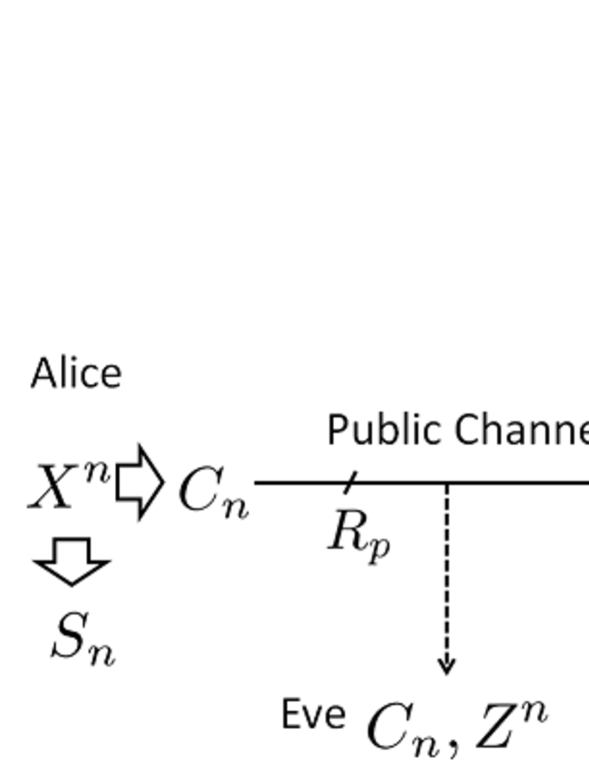
Figure 2: The key agreement protocol with one-way public communication. First, Alice sends the message $C_{n}$ to Bob over the public channel, which might be eavesdropped by Eve. Then, Alice compute the key $S_{n}$ and Bob compute the key $S_{n}^{\prime}$. The rate of the public communication is limited by $R_{p}$.

The error probability of the protocol is defined by

$$\varepsilon_{n}:=\Pr\{S_{n}\neq S_{n}^{\prime}\}.$$

The security of the protocol is measured by the quantity

$$\nu_{n}:=\log|{\cal S}_{n}|-H(S_{n}|C_{n},Z^{n}),$$

where ${\cal S}_{n}$ is the range of the key $S_{n}$.

In this paper, we are interested in the trade-off between the public communication rate $R_{p}$ and the key rate $R_{k}$. The rate pair $(R_{p},R_{k})$ is defined to be achievable if there exists a sequence of protocols satisfying

$$\lim_{n\to\infty}\varepsilon_{n} = 0,$$

$$\lim_{n\to\infty}\nu_{n} = 0,$$

$$\limsup_{n\to\infty}\frac{1}{n}\log|{\cal C}_{n}| \leq R_{p},$$

$$\liminf_{n\to\infty}\frac{1}{n}\log|{\cal S}_{n}| \geq R_{k},$$

where ${\cal C}_{n}$ is the range of the message $C_{n}$ transmitted over the public channel. Then, the achievable rate region is defined as

$${\cal R}(X,Y,Z):=\{(R_{p},R_{k}):\mbox{$(R_{p},R_{k})$ is achievable}\}.$$

In [20], the authors showed a closed form expression of ${\cal R}(X,Y,Z)$ for the scalar problem, i.e., $m_{x}=m_{y}=m_{z}=1$. In the next section, we show that the achievable rate region for the vector problem can be characterized as a (covariance) matrix optimization problem.

III Main Result

III-A Main Theorems

In this section, we show our main results. Since the security quantities $\varepsilon_{n}$ and $\nu_{n}$ only depend on the marginal distributions of $(X,Y)$ and $(X,Z)$ respectively, it suffice to consider $(X,Y,Z)$ of the form

$$Y = BX+W_{y},$$

$$Z = EX+W_{z},$$

where $B\in\mathbb{R}^{m_{y}\times m_{x}}$, $E\in\mathbb{R}^{m_{z}\times m_{x}}$, $W_{y}\sim{\cal N}(0,I_{m_{y}})$ and $W_{z}\sim{\cal N}(0,I_{m_{z}})$. In the rest of this paper, we omit the subscript of the identity matrix if the dimension is obvious from the context.

One of the main results of this paper is the following.

Theorem 1

Let ${\cal R}_{G}(X,Y,Z)$ be the set of all rate pairs $(R_{p},R_{k})$ satisfying

$$R_{p} \geq \frac{1}{2}\log\left|\frac{\Sigma_{x}}{\Sigma_{x|u}}\right|-\frac{1}{2}\log\left|\frac{B\Sigma_{x}B^{T}+I}{B\Sigma_{x|u}B^{T}+I}\right|,$$

$$R_{k} \leq \frac{1}{2}\log\left|\frac{B\Sigma_{x}B^{T}+I}{B\Sigma_{x|u}B^{T}+I}\right|-\frac{1}{2}\log\left|\frac{E\Sigma_{x}E^{T}+I}{E\Sigma_{x|u}E^{T}+I}\right|$$

for some $0\prec\Sigma_{x|u}\preceq\Sigma_{x}$. Then, we have

$${\cal R}(X,Y,Z)={\cal R}_{G}(X,Y,Z).$$

We are also interested in the asymptotic behavior of the function

$$R_{k}(R_{p}):=\sup\{R_{k}:~{}(R_{p},R_{k})\in{\cal R}(X,Y,Z)\}.$$ (1)

Following the approach in [11], we can obtain a closed form expression of $\lim_{R_{p}\to\infty}R_{k}(R_{p})$ as follows. Let $\phi_{i},i=1,\ldots,m_{x}$ be the generalized eigenvalues [23, Chapter 6.3] of the matrices

$$\left(\Sigma_{x}^{\frac{1}{2}}B^{T}B\Sigma_{x}^{\frac{1}{2}}+I_{m_{x}},\Sigma_{x}^{\frac{1}{2}}E^{T}E\Sigma_{x}^{\frac{1}{2}}+I_{m_{x}}\right).$$

Without loss of generality, we may assume that these generalized eigenvalues are ordered as

$$\phi_{1}\geq\cdots\geq\phi_{\rho}>1\geq\phi_{\rho+1}\geq\cdots\geq\phi_{m_{x}},$$ (2)

i.e., a total of $\rho$ of them are assumed to be greater than $1$. Then, we have

$$\lim_{R_{p}\to\infty}R_{k}(R_{p}) = \max_{0\preceq\Sigma_{x|u}\preceq\Sigma_{x}}\left[\frac{1}{2}\log\left|\frac{B\Sigma_{x}B^{T}+I}{B\Sigma_{x|u}B^{T}+I}\right|\right.$$ (3)

$$\left.~{}~{}~{}~{}~{}~{}~{}~{}~{}~{}~{}~{}~{}-\frac{1}{2}\log\left|\frac{E\Sigma_{x}E^{T}+I}{E\Sigma_{x|u}E^{T}+I}\right|\right]$$

$$= \frac{1}{2}\sum_{i=1}^{\rho}\log\phi_{i}.$$

Since Eq. (3) can be proved almost in the same manner as [11, Theorem 3], we omit a proof.

When $m_{x}=m_{y}=m_{z}$ and both $B$ and $E$ are invertible, it suffice to consider the case in which

$$Y = X+W_{y},$$ (4)

$$Z = X+W_{z},$$ (5)

where the covariance matrices $\Sigma_{W_{y}}$ and $\Sigma_{W_{z}}$ are not necessarily identity but are invertible. Following [22], we call this case the aligned case. As is usual with the vector Gaussian problems (e.g. [22]), the general statement (Theorem 1) is shown by detouring the statement for the aligned case.

Theorem 2

Let ${\cal R}^{*}_{G}(X,Y,Z)$ be the set of all rate pairs $(R_{p},R_{k})$ satisfying

$$R_{p} \geq I_{p}(\Sigma_{x|u})$$

$$:= \frac{1}{2}\log\left|\frac{\Sigma_{x}}{\Sigma_{x|u}}\right|-\frac{1}{2}\log\left|\frac{\Sigma_{x}+\Sigma_{W_{y}}}{\Sigma_{x|u}+\Sigma_{W_{y}}}\right|,$$

$$R_{k} \leq I_{k}(\Sigma_{x|u})$$

$$:= \frac{1}{2}\log\left|\frac{\Sigma_{x}+\Sigma_{W_{y}}}{\Sigma_{x|u}+\Sigma_{W_{y}}}\right|-\frac{1}{2}\log\left|\frac{\Sigma_{x}+\Sigma_{W_{z}}}{\Sigma_{x|u}+\Sigma_{W_{z}}}\right|$$

for some $0\prec\Sigma_{x|u}\preceq\Sigma_{x}$. Then, we have

$${\cal R}(X,Y,Z)={\cal R}^{*}_{G}(X,Y,Z).$$

Theorem 2 is shown in Section IV and Theorem 1 is shown in Section V by using Theorem 2.

III-B Numerical Examples

In this section, we show some numerical example to illustrate Theorem 1. In general, calculation of ${\cal R}_{G}(X,Y,Z)$ involves a nonconvex optimization problem and is not tractable. However for $m_{x}\geq 2$ and $m_{y}=m_{z}=1$, following the method in [24] (see also [10]), we can transform the calculation of ${\cal R}_{G}(X,Y,Z)$ into tractable form.

For $m_{x}\geq 2$ and $m_{y}=m_{z}=1$, we have

$$I_{p}(\Sigma_{x|u}) = \frac{1}{2}\log\left|\frac{\Sigma_{x}}{\Sigma_{x|u}}\right|-\frac{1}{2}\log\frac{b\Sigma_{x}b^{T}+1}{b\Sigma_{x|u}b^{T}+1},$$

$$I_{k}(\Sigma_{x|u}) = \frac{1}{2}\log\frac{b\Sigma_{x}b^{T}+1}{b\Sigma_{x|u}b^{T}+1}-\frac{1}{2}\log\frac{e\Sigma_{x}e^{T}+1}{e\Sigma_{x|u}e^{T}+1},$$

where $b,e\in\mathbb{R}^{m_{x}}$. Noting the relation

$$\frac{e\Sigma_{x|u}e^{T}+1}{b\Sigma_{x|u}b^{T}+1}=1+\frac{e\Sigma_{x|u}e^{T}-b\Sigma_{x|u}b^{T}+1}{b\Sigma_{x|u}b^{T}+1},$$

we set

$$s = b\Sigma_{x|u}b^{T},$$

$$t = \frac{e\Sigma_{x|u}e^{T}-b\Sigma_{x|u}b^{T}+1}{b\Sigma_{x|u}b^{T}+1}.$$

Let

$$I_{p}(\Sigma_{x|u},s) := \frac{1}{2}\log\left|\frac{\Sigma_{x}}{\Sigma_{x|u}}\right|-\frac{1}{2}\log(b\Sigma_{x}b^{T}+1)$$

$$~{}~{}~{}~{}~{}~{}~{}~{}~{}~{}~{}~{}~{}~{}~{}~{}+\frac{1}{2}\log(1+s),$$

$$I_{k}(t) = \frac{1}{2}\log\frac{b\Sigma_{x}b^{T}+1}{e\Sigma_{x}e^{T}+1}+\frac{1}{2}\log(1+t).$$

Then we can easily find that

$${\cal R}_{G}(X,Y,Z)$$

$$=\{(R_{p},R_{k}):~{}R_{p} \geq I_{p}(\Sigma_{x|u},s),$$

$$R_{k} \leq I_{k}(t),$$

$$0\prec\Sigma_{x|u} \preceq \Sigma_{x},$$

$$t(b\Sigma_{x|u}b^{T}+1) \leq e\Sigma_{x|u}e^{T}-b\Sigma_{x|u}b^{T},$$

$$b\Sigma_{x|u}b^{T} \leq s\}.$$

For fixed $(s,t)$, the optimization problem

minimize $$I_{p}(\Sigma_{x|u},s)$$

subject to $$t(b\Sigma_{x|u}b^{T}+1)\leq e\Sigma_{x|u}e^{T}-b\Sigma_{x|u}b^{T}$$

$$b\Sigma_{x|u}b^{T}\leq s$$

$$0\prec\Sigma_{x|u}\preceq\Sigma_{x}$$

is a convex problem. By sweeping $(s,t)$, we can calculate the region ${\cal R}_{G}(X,Y,Z)$.

For

$$\Sigma_{x}=\left[\begin{array}[]{cc}2&0\\ 0&2\end{array}\right],~{}b=\left[\begin{array}[]{cc}1&0.5\end{array}\right],~{}e=\left[\begin{array}[]{cc}0.7&0.35\end{array}\right],$$ (10)

the region ${\cal R}_{G}(X,Y,Z)$ is plotted in Fig. 3. Note that this case is degraded in the sense of [25, Definition 1], i.e., $X\leftrightarrow Y\leftrightarrow Z$ by appropriately choosing the correlation between $(Y,Z)$. In this case, the function $R_{k}(R_{p})$ converges to $I(X;Y)-I(X;Z)$ as $R_{p}$ increases.

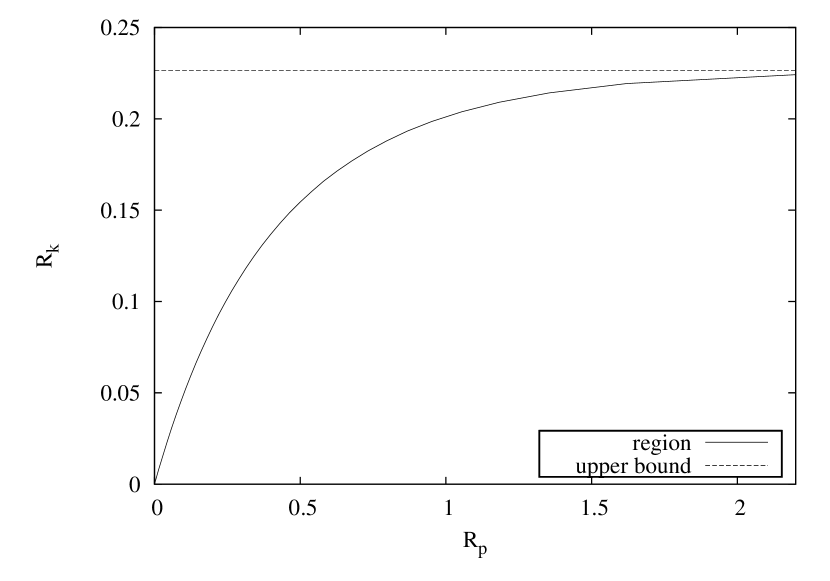
Figure 3: ”region“ is $R_{k}(R_{p})$ defined in Eq. (1) for the sources given by Eq. (10). ”upper bound” is the quantity $I(X;Y)-I(X;Z)$.

For

$$\Sigma_{x}=\left[\begin{array}[]{cc}2&0\\ 0&2\end{array}\right],~{}b=\left[\begin{array}[]{cc}1&0.5\end{array}\right],~{}e=\left[\begin{array}[]{cc}0.5&1\end{array}\right],$$ (15)

the region ${\cal R}_{G}(X,Y,Z)$ is plotted in Fig. 4. Note that $(X,Y,Z)$ in this example is not degraded. Although $I(X;Y)-I(X;Z)=0$ in this example, Fig. 4 clarifies that appropriate quantization enables Alice and Bob to share a secret key at positive key rate.

Figure 4: ”region“ is $R_{k}(R_{p})$ defined in Eq. (1) for the sources given by Eq. (15). “upper bound is $\lim_{R_{p}\to\infty}R_{k}(R_{p})$ which is explicitly given by Eq. (3).

For non-degraded case, $R_{k}(R_{p})$ converges to the quantity given by Eq. (3) instead of $I(X;Y)-I(X;Z)$ as $R_{p}$ increases, and it is also plotted in Fig. 4.

IV Proof of Theorem 2

IV-A Direct Part

In [20], the present authors proved the following proposition, which is an extension of [2, Theorem 2.6] to continuous sources.

Proposition 3

For an auxiliary random variable $U$ satisfying the Markov chain

$$U\leftrightarrow X\leftrightarrow(Y,Z),$$

let $(R_{p},R_{k})$ be a rate pair such that

$$R_{p} \geq I(U;X)-I(U;Y),$$

$$R_{k} \leq I(U;Y)-I(U;Z).$$

Then, we have $(R_{p},R_{k})\in{\cal R}(X,Y,Z)$.

The direct part of Theorem 2 is shown by taking Gaussian auxiliary random variable $U$ such that the conditional covariance matrix of $X$ given $U$ is $\Sigma_{x|u}$ in Proposition 3. ∎

IV-B Converse Part

In the converse proof, we will use the following Proposition and Corollary. The proposition was shown for discrete sources in [2, Theorem 2.6], and it can be shown almost in the same manner for continuous sources.

Proposition 4

([2]) Suppose that a rate pair $(R_{p},R_{k})$ is included in ${\cal R}(X,Y,Z)$. Then, there exist auxiliary random variables $U$ and $V$ satisfying

$$R_{p} \geq I(U;X|Y),$$ (16)

$$R_{k} \leq I(U;Y|V)-I(U;Z|V),$$ (17)

and the Markov chain

$$V\leftrightarrow U\leftrightarrow X\leftrightarrow(Y,Z).$$ (18)

For degraded sources, we can simplify the above proposition (see [20, Appendix B] for a proof).

Corollary 5

Suppose that $(X,Y,Z)$ is degraded, i.e., $X\leftrightarrow Y\leftrightarrow Z$. If $(R_{p},R_{k})\in{\cal R}(X,Y,Z)$, then there exists an auxiliary random variable $U$ satisfying

$$R_{p} \geq I(U;X|Y)=I(U;X)-I(U;Y),$$ (19)

$$R_{k} \leq I(U;Y|Z)=I(U;Y)-I(U;Z),$$ (20)

and the Markov chain

$$U\leftrightarrow X\leftrightarrow Y\leftrightarrow Z.$$ (21)

We show a converse proof of Theorem 2 by contradiction. Suppose that there exists a rate pair such that $(R_{p}^{o},R_{k}^{o})\in{\cal R}(X,Y,Z)$ and $(R_{p}^{o},R_{k}^{o})\notin{\cal R}_{G}^{*}(X,Y,Z)$, where we assume $R_{k}^{o}>0$ to avoid the trivial case. Then, there exists $0\prec\Sigma_{x|u}^{o}\preceq\Sigma_{x}$ such that $I_{p}(\Sigma_{x|u}^{o})\leq R_{p}^{o}$. Therefore, we can write

$$R_{k}^{o}=R_{k}^{*}+\delta$$ (22)

for some $\delta>0$, where $R_{k}^{*}$ is given by the optimal value of

maximize $$I_{k}(\Sigma_{x|u})$$

subject to $$I_{p}(\Sigma_{x|u})\leq R_{p}^{o},$$

$$0\prec\Sigma_{x|u}\preceq\Sigma_{x}.$$

An optimal solution $\Sigma_{x|u}^{*}$ of this optimization problem satisfies the Karash-Kuhn-Tucker (KKT) condition (see Appendix A for the derivation)

$$\mu(\Sigma_{x|u}^{*})^{-1} + (\Sigma_{x|u}^{*}+\Sigma_{W_{z}})^{-1}$$

$$= (1+\mu)(\Sigma_{x|u}^{*}+\Sigma_{W_{y}})^{-1}+M,$$

$$M(\Sigma_{x}-\Sigma_{x|u}^{*}) = 0,$$ (25)

$$\mu(R_{p}^{o}-I_{p}(\Sigma_{x|u}^{*})) = 0,$$ (26)

where $\mu\geq 0$ and $M\succeq 0$. From Eqs. (22) and (26), we have

$$R_{k}^{o}-\mu R_{p}^{o}=I_{k}(\Sigma_{x|u}^{*})-\mu I_{p}(\Sigma_{x|u}^{*})+\delta.$$ (27)

We shall find a contradiction to Eq. (27) by showing that for any $(R_{p},R_{k})\in{\cal R}(X,Y,Z)$

$$R_{k}-\mu R_{p}\leq I_{k}(\Sigma_{x|u}^{*})-\mu I_{p}(\Sigma_{x|u}^{*}).$$ (28)

The proof of Eq. (28) roughly consists of three steps: In the first step, we reduce the proof for the non-degraded sources to that for the degraded sources by using the enhancement technique introduced by Weingarten et. al. [22]. In the second step, we change the variable so that we can use the entropy power inequality (EPI). In the last step, we derive an upper bound on $R_{k}-\mu R_{p}$ by using the EPI, which turn out to be tight.

Step 1: In this step, in order to reduce the proof for the non-degraded sources to that for the degraded sources, we introduce the covariance matrix $\Sigma_{\tilde{W}_{y}}$ satisfying

$$(1+\mu)(\Sigma_{x|u}^{*}+\Sigma_{\tilde{W}_{y}})^{-1}$$ (29)

$$= (1+\mu)(\Sigma_{x|u}^{*}+\Sigma_{W_{y}})^{-1}+M.$$

Then, we have (see Appendix B for a proof)

$$0\prec\Sigma_{\tilde{W}_{y}}\preceq\Sigma_{W_{y}},$$ (30)

$$\Sigma_{\tilde{W}_{y}}\preceq\Sigma_{W_{z}}.$$ (31)

Let $\tilde{W}_{y}$ be the Gaussian random vector whose covariance matrix is $\Sigma_{\tilde{W}_{y}}$, and let

$$\tilde{Y}=X+\tilde{W}_{y}.$$ (32)

From Eq. (31), we can find that the sources $(X,\tilde{Y},Z)$ satisfy $X\leftrightarrow\tilde{Y}\leftrightarrow Z$. Furthermore, from Eq. (30), we can also find that $X\leftrightarrow\tilde{Y}\leftrightarrow Y$, which implies

$${\cal R}(X,Y,Z)\subset{\cal R}(X,\tilde{Y},Z).$$

Thus, it suffice to show that Eq. (28) holds for any $(R_{p},R_{k})\in{\cal R}(X,\tilde{Y},Z)$. In steps 2 and 3, we will show that

$$R_{k}-\mu R_{p}\leq\tilde{I}_{k}(\Sigma_{x|u}^{*})-\mu\tilde{I}_{p}(\Sigma_{x|u}^{*})$$ (33)

for any $(R_{p},R_{k})\in{\cal R}(X,\tilde{Y},Z)$, where

$$\tilde{I}_{p}(\Sigma_{x|u}) := \frac{1}{2}\log\left|\frac{\Sigma_{x}}{\Sigma_{x|u}}\right|-\frac{1}{2}\log\left|\frac{\Sigma_{x}+\Sigma_{\tilde{W}_{y}}}{\Sigma_{x|u}+\Sigma_{\tilde{W}_{y}}}\right|,$$

$$\tilde{I}_{k}(\Sigma_{x|u}) := \frac{1}{2}\log\left|\frac{\Sigma_{x}+\Sigma_{\tilde{W}_{y}}}{\Sigma_{x|u}+\Sigma_{\tilde{W}_{y}}}\right|-\frac{1}{2}\log\left|\frac{\Sigma_{x}+\Sigma_{W_{z}}}{\Sigma_{x|u}+\Sigma_{W_{z}}}\right|.$$

Then, by using the relation (see Appendix C for a proof)

$$(\Sigma_{x}+\Sigma_{\tilde{W}_{y}})(\Sigma_{x|u}^{*}+\Sigma_{\tilde{W}_{y}})^{-1}$$ (34)

$$= (\Sigma_{x}+\Sigma_{W_{y}})(\Sigma_{x|u}^{*}+\Sigma_{W_{y}})^{-1},$$

we have $I_{k}(\Sigma_{x|u}^{*})=\tilde{I}_{k}(\Sigma_{x|u}^{*})$ and $I_{p}(\Sigma_{x|u}^{*})=I_{p}(\Sigma_{x|u}^{*})$. Thus, Eq. (33) implies that Eq. (28) holds for any $(R_{p},R_{k})\in{\cal R}(X,\tilde{Y},Z)$.

Step 2: First, we show Eq. (33) for $\mu=0$. In this case, from Eqs. (LABEL:eq:kkt-1) and (29), we have $\Sigma_{\tilde{W}_{y}}=\Sigma_{W_{z}}$. Thus, from Corollary 5, we have

$$R_{k}-0\cdot R_{p}\leq I(U;Y)-I(U;Z)=0=\tilde{I}_{k}(\Sigma_{x|u}^{*}).$$

Thus, we have the assertion.

In order to prove Eq. (33) for $\mu>0$, we change the variable as follows. Since $(X,\tilde{Y},Z)$ is jointly Gaussian, we can write

$$X = K_{xz}Z+N_{1},$$

$$\tilde{Y} = K_{\tilde{y}x}X+K_{\tilde{y}z}Z+N_{2}$$

for Gaussian random vectors $N_{1},N_{2}$ with covariance matrices

$$\Sigma_{N_{1}} = \Sigma_{x|z}:=\Sigma_{x}-K_{xz}\Sigma_{zx},$$

$$\Sigma_{N_{2}} = \Sigma_{\tilde{y}|xz}:=\Sigma_{\tilde{y}}-K_{\tilde{y}x}\Sigma_{x\tilde{y}}-K_{\tilde{y}z}\Sigma_{z\tilde{y}},$$

where the coefficients are given by

$$K_{xz}=\Sigma_{xz}\Sigma_{z}^{-1}$$

and

$$\left[\begin{array}[]{cc}K_{\tilde{y}z}&K_{\tilde{y}x}\end{array}\right]=\left[\begin{array}[]{cc}\Sigma_{\tilde{y}z}&\Sigma_{\tilde{y}x}\end{array}\right]\left[\begin{array}[]{cc}\Sigma_{z}&\Sigma_{zx}\\ \Sigma_{xz}&\Sigma_{x}\end{array}\right]^{-1}.$$ (39)

By noting the relations

$$I(U;X|\tilde{Y}) = I(U;X)-I(U;\tilde{Y}),$$

$$I(U;\tilde{Y}|Z) = I(U;\tilde{Y})-I(U;Z),$$

$$I(U;X|Z) = I(U;X)-I(U;Z),$$

$$I(U;X|\tilde{Y}) = I(U;X|Z)-I(U;\tilde{Y}|Z)$$

for random variables satisfying $U\leftrightarrow X\leftrightarrow\tilde{Y}\leftrightarrow Z$, we have

$$\tilde{I}_{k}(\Sigma_{x|u})-\mu\tilde{I}_{p}(\Sigma_{x|u})$$

$$= I(U;\tilde{Y}|Z)-\mu I(U;X|\tilde{Y})$$

$$= (1+\mu)I(U;\tilde{Y}|Z)-\mu I(U;X|Z)$$

$$= [(1+\mu)h(\tilde{Y}|Z)-\mu h(X|Z)]$$

$$+[\mu h(X|U,Z)-(1+\mu)h(\tilde{Y}|U,Z)]$$

$$= [(1+\mu)h(\tilde{Y}|Z)-\mu h(X|Z)]-\frac{1+\mu}{2}\log|K_{\tilde{y}x}K_{\tilde{y}x}^{T}|$$

$$+\mu[h(X|U,Z)-\gamma h(X+K_{\tilde{y}x}^{-1}N_{2}|U,Z)]$$

$$= [(1+\mu)h(\tilde{Y}|Z)-\mu h(X|Z)]-\frac{1+\mu}{2}\log|K_{\tilde{y}x}K_{\tilde{y}x}^{T}|$$

$$+\mu[h(X|U,Z)-\gamma h(X+N_{3}|U,Z)]$$

$$= [(1+\mu)h(\tilde{Y}|Z)-\mu h(X|Z)]-\frac{1+\mu}{2}\log|K_{\tilde{y}x}K_{\tilde{y}x}^{T}|$$

$$+ \mu\left[\frac{1}{2}\log(2\pi e)^{m}|\Sigma_{x|uz}|-\frac{\gamma}{2}\log(2\pi e)^{m}|\Sigma_{x|uz}+\Sigma_{N_{3}}|\right],$$

where we set $\gamma:=\frac{1+\mu}{\mu}>1$ and $N_{3}:=K_{\tilde{y}x}^{-1}N_{2}$. It should be noted that

$$|K_{\tilde{y}x}|\neq 0$$ (41)

for $\mu>0$, which will be proved in Appendix D.

For the change of variable

$$\phi:\Sigma_{x|u}\mapsto\Sigma_{x|uz}=(\Sigma_{x|u}^{-1}+\Sigma_{W_{z}}^{-1})^{-1},$$

let $\Sigma_{x|uz}^{*}:=\phi(\Sigma_{x|u}^{*})$. From Eqs. (LABEL:eq:kkt-1) and (29) and the relation

$$\tilde{I}_{k}(\Sigma_{x|u})-\mu\tilde{I}_{p}(\Sigma_{x|u})$$

$$= \frac{\mu}{2}\log(2\pi e)^{m}|\Sigma_{x|u}|+\frac{1}{2}\log(2\pi e)^{m}|\Sigma_{x|u}+\Sigma_{W_{z}}|$$

$$~{}~{}~{}~{}~{}~{}-\frac{(1+\mu)}{2}\log(2\pi e)^{m}|\Sigma_{x|u}+\Sigma_{\tilde{W}_{y}}|$$

$$+[(1+\mu)h(\tilde{Y})-h(Z)-\mu h(X)],$$

we have

$$\nabla_{\Sigma_{x|u}}\left[\tilde{I}_{k}(\Sigma_{x|u}^{*})-\mu\tilde{I}_{p}(\Sigma_{x|u}^{*})\right]=0.$$

By the chain rule for the derivative, we have

$$\nabla_{\Sigma_{x|uz}}\left[\tilde{I}_{k}(\phi^{-1}(\Sigma_{x|uz}^{*}))-\mu\tilde{I}_{p}(\phi^{-1}(\Sigma_{x|uz}^{*}))\right]$$

$$= \nabla_{\Sigma_{x|uz}}\phi^{-1}(\Sigma_{x|uz}^{*})\cdot\nabla_{\Sigma_{x|u}}\left[\tilde{I}_{k}(\Sigma_{x|u}^{*})-\mu\tilde{I}_{p}(\Sigma_{x|u}^{*})\right]$$

$$= 0.$$

Thus, from Eq. (LABEL:eq:variable-changed), we have

$$(\Sigma_{x|uz}^{*})^{-1}=\gamma(\Sigma_{x|uz}^{*}+\Sigma_{N_{3}})^{-1}.$$ (42)

Step 3: By noting that $(X,\tilde{Y},Z)$ is degraded, from Corollary 5, for any $(R_{p},R_{k})\in{\cal R}(X,\tilde{Y},Z)$ we have

$$R_{k}-\mu R_{p}$$ (43)

$$\leq I(U;\tilde{Y}|Z)-\mu I(U;X|\tilde{Y})$$

$$= [(1+\mu)h(\tilde{Y}|Z)-\mu h(X|Z)]-\frac{1+\mu}{2}\log|K_{\tilde{y}x}K_{\tilde{y}x}^{T}|$$

$$+\mu\left[h(X|U,Z)-\gamma h(X+N_{3}|U,Z)\right],$$

where $U$ is not necessarily Gaussian. By using the conditional version of EPI [26], we have

$$h(X|U,Z)-\gamma h(X+N_{3}|U,Z)$$

$$\leq h(X|U,Z)$$

$$-\frac{\gamma m}{2}\log\left(\exp\left[\frac{2}{m}h(X|U,Z)\right]+\exp\left[\frac{2}{m}h(N_{3})\right]\right)$$

$$\leq f\left(h(N_{3})-\frac{m}{2}\log(\gamma-1);h(N_{3})\right),$$ (45)

where we set

$$f(t;a):=t-\frac{\gamma m}{2}\log\left(\exp\left[\frac{2}{m}t\right]+\exp\left[\frac{2}{m}a\right]\right).$$

Note that the function $f(t;a)$ is concave function of $t$ and takes the maximum at $t=a-\frac{m}{2}\log(\gamma-1)$ [27]. From Eq. (42), we have

$$(\gamma-1)^{-1}\Sigma_{N_{3}}=\Sigma_{x|uz}^{*},$$

which implies

$$h(N_{3})-\frac{m}{2}\log(\gamma-1) = \frac{1}{2}\log(2\pi e)^{m}(\gamma-1)^{-m}|\Sigma_{N_{3}}|$$

$$= \frac{1}{2}\log(2\pi e)^{m}|\Sigma_{x|uz}^{*}|.$$

Furthermore, since $\Sigma_{x|uz}^{*}$ and $\Sigma_{N_{3}}$ are proportional to each other, we have

$$|\Sigma_{x|uz}^{*}|^{1/m}+|\Sigma_{N_{3}}|^{1/m}=|\Sigma_{x|uz}^{*}+\Sigma_{N_{3}}|^{1/m}.$$

Thus, from Eqs. (43) and (45), we have

$$R_{k}-\mu R_{p}$$

$$\leq [(1+\mu)h(\tilde{Y}|Z)-\mu h(X|Z)]-\frac{1+\mu}{2}\log|K_{\tilde{y}x}K_{\tilde{y}x}^{T}|$$

$$+\mu\left[\frac{1}{2}\log(2\pi e)^{m}|\Sigma_{x|uz}^{*}|-\frac{\gamma}{2}\log(2\pi e)^{m}|\Sigma_{x|uz}^{*}+\Sigma_{N_{3}}|\right]$$

$$= \tilde{I}_{k}(\Sigma_{x|u}^{*})-\mu\tilde{I}_{p}(\Sigma_{x|u}^{*}).$$

∎

Remark 6

One of the difficulties in the above proof is that, after Step 1, we have to show the extremal inequality of the form

$$\mu h(X|U)+h(X+W_{z}|U)-(1+\mu)h(X+\tilde{W}_{y}|U)$$ (46)

$$\leq \frac{\mu}{2}\log|\Sigma_{x|u}^{*}|+\frac{1}{2}\log|\Sigma_{x|u}^{*}+\Sigma_{W_{z}}|$$

$$~{}~{}~{}~{}~{}-\frac{(1+\mu)}{2}\log|\Sigma_{x|u}^{*}+\Sigma_{\tilde{W}_{y}}|.$$

This type of extremal inequality has appeared in [28, Corollary 2] (scalar version has appeared in [29, Lemma 1]). In [14], the extremal inequality was proved by using a vector generalization of Costa’s entropy power inequality [30]. On the otherhand, we showed Eq. (46) by using the change of variable in Step 2 and by reducing to more tractable form (Eq. (IV-B)), which has appeared in the literature [27]. By this reduction, we only need the standard EPI in our proof instead of Costa’s type EPI, and our proof seems more elementary.

V Proof of Theorem 1

In this section, we show Theorem 1 by using Theorem 2. We follow a similar approach as in [10, Section 4]. Since the direct part can be proved by taking a Gaussian auxiliary random variable $U$ in Proposition 3 (see Section IV-A), we concentrate on the converse part. Without loss of generality, we can assume that the matrices $B$ and $E$ are square (but not necessarily invertible). If that is not the case, we can apply singular value decomposition (SVD) to show equivalent sources $(X^{\prime},Y^{\prime},Z^{\prime})$ on $\mathbb{R}^{m_{x}}\times\mathbb{R}^{m_{x}}\times\mathbb{R}^{m_{x}}$ such that ${\cal R}(X^{\prime},Y^{\prime},Z^{\prime})={\cal R}(X,Y,Z)$ in a similar manner as [22, Section 5-B].

By using SVD, we can write the matrices as

$$B = U_{y}\Lambda_{y}V_{y},$$

$$E = U_{z}\Lambda_{z}V_{z},$$

where $U_{y},V_{y},U_{z}$ and $V_{z}$ are $m_{x}\times m_{x}$ orthogonal matrices, and $\Lambda_{y}$ and $\Lambda_{z}$ are diagonal matrices. Let

$$\bar{B} = U_{y}(\Lambda_{y}+\alpha I)V_{y},$$

$$\bar{E} = U_{y}(\Lambda_{z}+\alpha I)V_{z}$$

for some $\alpha>0$. Then, let

$$\bar{Y} = \bar{B}X+W_{y},$$

$$\bar{Z} = \bar{E}X+W_{z}.$$

Since $\bar{B}$ and $\bar{E}$ are invertible, Theorem 2 implies

$${\cal R}(X,\bar{Y},\bar{Z})={\cal R}_{G}(X,\bar{Y},\bar{Z}).$$ (47)

In the following, we will show the following lemma.

Lemma 7

We have

$${\cal R}(X,Y,Z)\subset{\cal R}(X,\bar{Y},\bar{Z})+{\cal O}(X,\bar{Y},\bar{Z}),$$

where

$${\cal O}(X,\bar{Y},\bar{Z}) = \left\{(0,R_{k}):0\leq R_{k}\leq\frac{1}{2}\log|\bar{E}\Sigma_{x}\bar{E}^{T}+I|\right.$$

$$\left.~{}~{}-\frac{1}{2}\log|E\Sigma_{x}E^{T}+I|\right\}.$$

By letting $\alpha\to 0$, ${\cal R}_{G}(X,\bar{X},\bar{Z})$ converges to ${\cal R}_{G}(X,Y,Z)$ and ${\cal O}(X,\bar{Y},\bar{Z})$ converges to $\{(0,0)\}$. Thus, Eq. (47) and Lemma 7 imply ${\cal R}(X,Y,Z)\subset{\cal R}_{G}(X,Y,Z)$.

Proof of Lemma 7

Let

$$C_{y} = U_{y}\Lambda_{y}(\Lambda_{y}+\alpha I)^{-1}V_{y},$$

$$C_{z} = U_{z}\Lambda_{z}(\Lambda_{z}+\alpha I)^{-1}V_{z}.$$

Then, we have $C_{y}C_{y}^{T}\prec I$ and $C_{z}C_{z}^{T}\prec I$. Thus, we can write

$$Y = C_{y}\bar{Y}+W_{y}^{\prime},$$

$$Z = C_{z}\bar{Z}+W_{z}^{\prime}$$

for $W_{y}^{\prime}\sim{\cal N}(0,I-C_{y}C_{y}^{T})$ and $W_{z}^{\prime}\sim{\cal N}(0,I-C_{z}C_{z}^{T})$, i.e., we have

$$X\leftrightarrow\bar{Y}\leftrightarrow Y,$$ (48)

$$X\leftrightarrow\bar{Z}\leftrightarrow Z.$$ (49)

From Proposition 4, for any $(R_{p},R_{k})\in{\cal R}(X,Y,Z)$, there exist $(U,V)$ satisfying

$$R_{p} \geq I(U;X)-I(U;Y),$$

$$R_{k} \leq I(U;Y|V)-I(U;Z|V),$$

and $(U,V)\leftrightarrow X\leftrightarrow(Y,Z)$. Let

$$\bar{R}_{p} = I(U;X)-I(U;\bar{Y}),$$

$$\bar{R}_{k} = I(U;\bar{Y}|V)-I(U;\bar{Z}|V).$$

Then, we have

$$R_{p}-\bar{R}_{p} \geq I(U;X)-I(U;Y)-[I(U;X)-I(U;\bar{Y})]$$

$$= I(U;\bar{Y})-I(U;Y)$$

$$\geq 0,$$

where the second inequality follows from Eq. (48). On the other hand, we have

$$R_{k}-\bar{R}_{k} \leq I(U;Y|V)-I(U;Z|V)$$

$$-[I(U;\bar{Y}|V)-I(U;\bar{Z}|V)]$$

$$= I(U;\bar{Z}|V)-I(U;Z|V)$$

$$-[I(U;\bar{Y}|V)-I(U;Y|V)]$$

$$\leq I(U;\bar{Z}|V)-I(U;Z|V)$$

$$= I(U,V;\bar{Z})-I(U,V;Z)$$

$$-[I(V;\bar{Z})-I(V;Z)]$$

$$\leq I(U,V;\bar{Z})-I(U,V;Z)$$

$$= I(X;\bar{Z})-I(X;Z)$$

$$-[I(X;\bar{Z}|U,V)-I(X;Z|U,V)]$$

$$\leq I(X;\bar{Z})-I(X;Z)$$

$$= \frac{1}{2}\log|\bar{E}\Sigma_{x}\bar{E}^{T}+I|-\frac{1}{2}\log|E\Sigma_{x}E^{T}+I|,$$

where the second, third, and forth inequalities follow from the Markov relations in Eqs. (48) and (49). ∎

VI Conclusion

In this paper, we investigated the secret key agreement from vector Gaussian sources by rate limited public communication. We characterized the optimal trade-off between the key rate and the public communication rate as a (covariance) matrix optimization problem. Investigating an efficient method to solve the optimization problem is a future research agenda.

Appendix A Derivation of the KKT condition

We first rewrite the optimization problem in Eq. (IV-B) as a standard form

minimize $$-I_{k}(\Sigma_{x|u})$$

subject to $$I_{p}(\Sigma_{x|u})-R_{p}^{o}\leq 0$$

$$0\prec\Sigma_{x|u}\preceq\Sigma_{x}.$$

Let $\Sigma_{x|u}^{*}$ be an optimal solution for this problem, which is also an optimal solution of Eq. (IV-B). Then, we have $\Sigma_{x|u}^{*}\succ 0$ because of the constraint $I_{p}(\Sigma_{x|u}^{*})-R_{p}^{o}\leq 0$. Thus, there exists a positive definite matrix $L$ satisfying $L\prec\Sigma_{x|u}^{*}$.

Let us consider another optimization problem

minimize $$-I_{k}(\Sigma_{x|u})$$

subject to $$I_{p}(\Sigma_{x|u})-R_{p}^{o}\leq 0$$

$$L\preceq\Sigma_{x|u}\preceq\Sigma_{x}.$$

Obviously, $\Sigma_{x|u}^{*}$ is also an optimal solution for the problem in Eq. (A), and the optimal values for Eqs. (A) and (A) are the same. Although the optimization problem in Eq. (A) is not convex, there exist Lagrange multipliers $M_{1}\succeq 0$, $M_{2}\succeq 0$, and $\mu\geq 0$ satisfying

$$-\left(-\nabla_{\Sigma_{x|u}}I_{k}(\Sigma_{x|u}^{*})+\mu\nabla_{\Sigma_{x|u}}(I_{p}(\Sigma_{x|u}^{*})-R_{p}^{o})\right)$$ (52)

$$= M_{2}-M_{1},$$

$$M_{1}(\Sigma_{x|u}^{*}-L) = 0,$$ (53)

$$M_{2}(\Sigma_{x}-\Sigma_{x|u}^{*})) = 0,$$ (54)

$$\mu(R_{p}-I_{p}(\Sigma_{x|u}^{*})) = 0$$ (55)

if the set of constraint qualifications (CQs) shown below are satisfied (see [22, Appendix 4] for the detail). Since $\Sigma_{x|u}^{*}\succ L$, Eq. (53) implies $M_{1}=0$. Thus, by noting the relation

$$I_{k}(\Sigma_{x|u})-\mu I_{p}(\Sigma_{x|u})$$ (56)

$$= \frac{\mu}{2}\log(2\pi e)^{m}|\Sigma_{x|u}|+\frac{1}{2}\log(2\pi e)^{m}|\Sigma_{x|u}+\Sigma_{W_{z}}|$$

$$~{}~{}~{}~{}~{}~{}-\frac{(1+\mu)}{2}\log(2\pi e)^{m}|\Sigma_{x|u}+\Sigma_{W_{y}}|$$

$$+[(1+\mu)h(Y)-h(Z)-\mu h(X)],$$

and by setting $M=2M_{2}$, we have the KKT conditions in Eqs. (LABEL:eq:kkt-1)–(26).

The CQs shown in [22, Appendix 4], which is an interpretation of [31, CQ5a of Section 5.4] are the following: There exists a matrix $A$ satisfying

1. For any $\mathbf{u}\neq 0$ in the null space of $\Sigma_{x|u}^{*}-L$, we have $\mathbf{u}^{T}A\mathbf{u}>0$.

2. For any $\mathbf{v}\neq 0$ in the null space of $\Sigma_{x}-\Sigma_{x|u}^{*}$, we have $\mathbf{v}^{T}A\mathbf{v}<0$.

3. $$\mathrm{Tr}\left[\nabla_{\Sigma_{x|u}}(I_{p}(\Sigma_{x|u}^{*})-R_{p}^{o})A^{T}\right]>0.$$

To check whether the above CQs are satisfied, we suggest $A$ given by

$$A=\alpha(L-\Sigma_{x|u}^{*})+(\Sigma_{x}-\Sigma_{x|u}^{*})$$

for $\alpha>0$. First we check (1). For any $\mathbf{u}\neq 0$ in the null space of $\Sigma_{x|u}^{*}-L$, we have

$$\mathbf{u}^{T}A\mathbf{u}=\mathbf{u}^{T}(\Sigma_{x}-\Sigma_{x|u}^{*})\mathbf{u}.$$

Suppose that $\mathbf{u}^{T}(\Sigma_{x}-\Sigma_{x|u}^{*})\mathbf{u}=0$. Then we have

$$0 = \mathbf{u}^{T}\left((\Sigma_{x|u}^{*}-L)+(\Sigma_{x}-\Sigma_{x|u}^{*})\right)\mathbf{u}$$

$$= \mathbf{u}^{T}(\Sigma_{x}-L)\mathbf{u},$$

which is a contradiction because $\Sigma_{x}\succ L$. Thus the condition (1) is satisfied.

Next, we check (2). For any $\mathbf{v}\neq 0$ in the null space of $\Sigma_{x}-\Sigma_{x|u}^{*}$, we have

$$\mathbf{v}^{T}A\mathbf{v}=\mathbf{v}^{T}(L-\Sigma_{x|u}^{*})\mathbf{v}<0$$

because $L\prec\Sigma_{x|u}^{*}$.

Finally, we check (3). By noting

$$\nabla_{\Sigma_{x|u}}I_{p}(\Sigma_{x|u})=\frac{1}{2}(\Sigma_{x|u}+\Sigma_{W_{y}})^{-1}-\frac{1}{2}\Sigma_{x|u}^{-1}\prec 0$$

for any $\Sigma_{x|u}\succ 0$, we have

$$\mathrm{Tr}\left[\nabla_{\Sigma_{x|u}}(I_{p}(\Sigma_{x|u}^{*})-R_{p}^{o})A\right]$$

$$= \frac{\alpha}{2}\mathrm{Tr}\left[\left\{(\Sigma_{x|u}^{*}+\Sigma_{W_{y}})^{-1}-(\Sigma_{x|u}^{*})^{-1}\right\}(L-\Sigma_{x|u}^{*})\right]$$

$$+\frac{1}{2}\mathrm{Tr}\left[\left\{(\Sigma_{x|u}^{*}+\Sigma_{W_{y}})^{-1}-(\Sigma_{x|u}^{*})^{-1}\right\}(\Sigma_{x}-\Sigma_{x|u}^{*})\right].$$

Since $L-\Sigma_{x|u}^{*}\prec 0$, by taking $\alpha>0$ to be sufficiently large, the condition (3) is satisfied.

Remark 8

We need to introduce the optimization problem in Eq. (A) because the arguments in [22, Appendix 4] is guaranteed only under the condition such that the range of the variable $\Sigma_{x|u}$ is a closed set.

Appendix B Proof of Eqs. (30) and (31)

By noting $M\succeq 0$, we have

$$(\Sigma_{x|u}^{*}+\Sigma_{\tilde{W}_{y}})^{-1} = (\Sigma_{x|u}^{*}+\Sigma_{W_{y}})^{-1}+M$$

$$\succeq (\Sigma_{x|u}^{*}+\Sigma_{W_{y}})^{-1}.$$

Thus we have

$$\Sigma_{\tilde{W}_{y}}\preceq\Sigma_{W_{y}}.$$

Since $\Sigma_{W_{z}}\succ 0$, by substituting Eq. (29) into Eq. (LABEL:eq:kkt-1), we have

$$(\Sigma_{x|u}^{*}+\Sigma_{\tilde{W}_{y}})^{-1}$$

$$= \frac{\mu}{1+\mu}(\Sigma_{x|u}^{*})^{-1}+\frac{1}{1+\mu}(\Sigma_{x|u}^{*}+\Sigma_{W_{z}})^{-1}$$

$$\prec (\Sigma_{x|u}^{*})^{-1}$$

when $\mu>0$. Thus, we have

$$\Sigma_{\tilde{W}_{y}}\succ 0.$$

Note that $\Sigma_{\tilde{W}_{y}}=\Sigma_{W_{z}}\prec 0$ when $\mu=0$.

From Eq. (B), we have

$$(\Sigma_{x|u}^{*}+\Sigma_{\tilde{W}_{y}})^{-1}\succeq(\Sigma_{x|u}^{*}+\Sigma_{W_{z}})^{-1},$$

where the strict inequality holds for $\mu>0$. Thus we have

$$\Sigma_{\tilde{W}_{y}}\preceq\Sigma_{W_{z}}$$

and especially

$$\Sigma_{\tilde{W}_{y}}\prec\Sigma_{W_{z}}$$ (58)

for $\mu>0$. ∎

Appendix C Proofs of Eq. (34)

Eq. (34) can be derived by the following sequence of equalities:

$$(\Sigma_{x}+\Sigma_{\tilde{W}_{y}})(\Sigma_{x|u}^{*}+\Sigma_{\tilde{W}_{y}})^{-1}$$ (59)

$$= \left[(\Sigma_{x}-\Sigma_{x|u}^{*})+(\Sigma_{x|u}^{*}+\Sigma_{\tilde{W}_{y}})\right](\Sigma_{x|u}^{*}+\Sigma_{\tilde{W}_{y}})^{-1}$$

$$= (\Sigma_{x}-\Sigma_{x|u}^{*})(\Sigma_{x|u}^{*}+\Sigma_{\tilde{W}_{y}})^{-1}+I$$

$$= (\Sigma_{x}-\Sigma_{x|u}^{*})\left[(\Sigma_{x|u}^{*}+\Sigma_{W_{y}})^{-1}+M\right]+I$$

$$= (\Sigma_{x}-\Sigma_{x|u}^{*})(\Sigma_{x|u}^{*}+\Sigma_{W_{y}})^{-1}+I$$

$$= \left[(\Sigma_{x}-\Sigma_{x|u}^{*})+(\Sigma_{x|u}^{*}+\Sigma_{W_{y}})\right](\Sigma_{x|u}^{*}+\Sigma_{W_{y}})^{-1}$$

$$= (\Sigma_{x}+\Sigma_{W_{y}})(\Sigma_{x|u}^{*}+\Sigma_{W_{y}})^{-1},$$ (61)

where Eq. (59) follows from Eq. (29) and Eq. (C) follows from Eq. (25).

Appendix D Proof of Eq. (41)

From Eqs. (32), (5) and (58), we can write

$$Z=X+\tilde{W}_{y}+W^{\prime},$$ (62)

where $W^{\prime}\sim{\cal N}(0,\Sigma_{\tilde{W}_{y}}-\Sigma_{W_{z}})$. Thus, we have

$$\Sigma_{\tilde{y}z} = \Sigma_{\tilde{y}},$$

$$\Sigma_{zx} = \Sigma_{xz}=\Sigma_{x}.$$

Furthermore, we have

$$\Sigma_{\tilde{y}}\prec\Sigma_{z}.$$ (63)

From the block inversion of the matrix (e.g. see [32, Appendix 5.5]) and Eq. (39), we have

$$K_{\tilde{y}x} = \left[\begin{array}[]{cc}\Sigma_{\tilde{y}}&\Sigma_{x}\end{array}\right]\left[\begin{array}[]{c}-\Sigma_{z}^{-1}\Sigma_{x}S^{-1}\\ S^{-1}\end{array}\right]$$ (67)

$$= (I-\Sigma_{\tilde{y}}\Sigma_{z}^{-1})\Sigma_{x}S^{-1},$$ (68)

where

$$S=\Sigma_{x}-\Sigma_{x}\Sigma_{z}^{-1}\Sigma_{x}$$

is the Schur complement.

From Eq. (63), we have

$$I-\Sigma_{\tilde{y}}^{\frac{1}{2}}\Sigma_{z}^{-1}\Sigma_{\tilde{y}}^{\frac{1}{2}}\succ I-\Sigma_{\tilde{y}}^{\frac{1}{2}}\Sigma_{\tilde{y}}^{-1}\Sigma_{\tilde{y}}^{\frac{1}{2}}=0.$$

Thus we have

$$|I-\Sigma_{\tilde{y}}\Sigma_{z}^{-1}|=|I-\Sigma_{\tilde{y}}^{\frac{1}{2}}\Sigma_{z}^{-1}\Sigma_{\tilde{y}}^{\frac{1}{2}}|\neq 0.$$ (69)

By combining Eqs. (68) and (69), we have Eq. (41). ∎

References

- [1] R. Ahlswede and I. Csiszár, “Common randomness in information theory and cryptography–part I: Secret sharing,” IEEE Trans. Inform. Theory, vol. 39, no. 4, pp. 1121–1132, July 1993.
- [2] I. Csiszár and P. Narayan, “Common randomness and secret key generation with a helper,” IEEE Trans. Inform. Theory, vol. 46, no. 2, pp. 344–366, March 2000.
- [3] ——, “Secrecy capacities for multiple terminals,” IEEE Trans. Inform. Theory, vol. 50, no. 12, pp. 3047–3061, December 2004.
- [4] U. Maurer, “Secret key agreement by public discussion from common information,” IEEE Trans. Inform. Theory, vol. 39, no. 3, pp. 733–742, May 1993.
- [5] A. D. Wyner, “The wire-tap channel,” Bell Syst. Tech. J., vol. 54, no. 8, pp. 1355–1387, 1975.
- [6] I. Csiszár and J. Körner, “Broadcast channels with confidential messages,” IEEE Trans. Inform. Theory, vol. 24, no. 3, pp. 339–348, May 1979.
- [7] Y. Liang, H. V. Poor, and S. Shamai, “Secure communication over fading channels,” IEEE Trans. Inform. Theory, vol. 54, no. 6, pp. 2470–2492, June 2008.
- [8] T. Liu and S. Shamai, “A note on the secrecy capacity of the multiple-antenna wiretap channel,” IEEE Trans. Inform. Theory, vol. 55, no. 6, pp. 2547–2553, June 2009.
- [9] R. Bustin, R. Liu, H. V. Poor, and S. Shamai, “An MMSE approach to the secrecy capacity of the MIMO Gaussian wiretap channel,” EURASIP Journal on Wireless Communication and Networking, 2009.
- [10] H. D. Ly, T. Liu, and Y. Liang, “Multiple-input multiple-output gaussian broadcast channels with common and confidential messages,” 2009, arXiv:0907.2599.
- [11] R. Liu, T. Liu, V. Poor, and S. Shamai (Shitz), “Multiple-input multiple-output gaussian broadcast channels with confidential messages,” 2009, arXiv:0903.3786.
- [12] E. Ekrem and S. Ulukus, “The secrecy capacity region of the gaussian MIMO multi-receiver wiretap channel,” 2009, arXiv:0903.3096v1.
- [13] ——, “Gaussian MIMO broadcast channels with common and confidential messages,” in Proc. IEEE Int. Symp. Inf. Theory 2010, Austin, U.S.A., 2010, pp. 2583–2587.
- [14] R. Liu, T. Liu, H. V. Poor, and S. Shamai (Shitz), “MIMO gaussian broadcast channels with confidential and common messages,” in Proc. IEEE Int. Symp. Inf. Theory 2010, Austin, U.S.A., 2010, pp. 2578–2582.
- [15] A. Khisti and G. W. Wornell, “Secure transmission with multiple antennas I:the misome wiretap channel,” IEEE Trans. Inform. Theory, vol. 56, no. 7, pp. 3088–3104, July 2010.
- [16] M. Bloch, J. Barros, M. R. D. Rodrigues, and S. W. McLaughlin, “Wireless information-theoretic security,” IEEE Trans. Inform. Theory, vol. 54, no. 6, pp. 2515–2534, June 2008.
- [17] F. Grosshans, G. V. Assche, J. Wenger, R. Brouri, N. J. Cerf, and P. Grangier, “Quantum key distribution using Gaussian-modulated coherent states,” Nature, vol. 421, pp. 238–241, January 2003.
- [18] G. V. Assche, J. Cardinal, and N. J. Cerf, “Reconciliation of a quantum-distributed Gaussian key,” IEEE Trans. Inform. Theory, vol. 50, no. 2, pp. 394–400, February 2004.
- [19] G. V. Assche, Quantum Cryptography and Secret-Key Distillation. Cambridge Univ. Press, 2006.
- [20] S. Watanabe and Y. Oohama, “Secret key agreement from correlated Gaussian sources by rate limited public communication,” IEICE Trans. Fundamentals (to be published), vol. E93A, no. 11, 2010, arXiv:1001.3705.
- [21] T. M. Cover and J. A. Thomas, Elements of Information Theory, 2nd ed. John Wiley & Sons, 2006.
- [22] H. Weingarten, Y. Steinberg, and S. Shamai (Shitz), “The capacity region of the Gaussian MIMO broadcast channel,” IEEE Trans. Inform. Theory, vol. 52, no. 9, pp. 3936–3964, September 2006.
- [23] G. Strang, Linear Algebra and Its Application. Wellesley-Cambridge Press, 1998.
- [24] H. Weingarten, Y. Steinberg, and S. Shamai (Shitz), “On the capacity region of the multi-antenna broadcast channel with common messages,” in Proc. IEEE Int. Symp. Inf. Theory 2006, Seattle, WA, 2006, pp. 2195–2199.
- [25] H. Weingarten, T. Liu, S. Shamai, Y. Steinberg, and P. Viswanath, “The capacity region of the degraded multiple-input multiple-output compound broadcast channel,” IEEE Trans. Inform. Theory, vol. 55, no. 11, pp. 5011–5023, November 2009.
- [26] P. P. Bergmans, “A simple converse for broadcast channels with additive white Gaussian noise,” IEEE Trans. Inform. Theory, vol. 20, no. 2, pp. 279–280, March 1974.
- [27] T. Liu and P. Viswanath, “An extremal inequality motivated by multiterminal information-theoretic problems,” IEEE Trans. Inform. Theory, vol. 53, no. 5, pp. 1839–1851, May 2007.
- [28] R. Liu, T. Liu, H. V. Poor, and S. Shamai (Shitz), “A vector generalization of costa’s entropy-power inequality with applications,” IEEE Trans. Inform. Theory, vol. 56, no. 4, pp. 1865–1879, April 2010.
- [29] J. Chen, “Rate region of gaussian multiple description coding with individual and central distortion constraints,” IEEE Trans. Inform. Theory, vol. 55, no. 9, pp. 3991–4005, September 2009.
- [30] M. H. M. Costa, “A new entropy power inequality,” IEEE Trans. Inform. Theory, vol. 31, no. 6, pp. 751–760, November 1985.
- [31] D. P. Bertsekas, A. Nedić, and A. E. Ozdaglar, Convex Analysis and Optimization. Athena Scientific, 2003.
- [32] S. Boyd and L. Vandenberghe, Convex Optimization. Cambridge University Press, 2004.