Face Detection with Effective Feature Extraction

Abstract

There is an abundant literature on face detection due to its important role in many vision applications. Since Viola and Jones proposed the first real-time AdaBoost based face detector, Haar-like features have been adopted as the method of choice for frontal face detection. In this work, we show that simple features other than Haar-like features can also be applied for training an effective face detector. Since, single feature is not discriminative enough to separate faces from difficult non-faces, we further improve the generalization performance of our simple features by introducing feature co-occurrences. We demonstrate that our proposed features yield a performance improvement compared to Haar-like features. In addition, our findings indicate that features play a crucial role in the ability of the system to generalize.

I Introduction

Face detection is an important first step for several computer vision applications. It was not until recently that face detection problem received considerable attention among researchers owing to the impressive performance of Viola and Jones’ face detector [1]. Their detector was the first algorithm that achieved real-time detection speed and high accuracy comparable to previous state of the art methods. Their work consists of three contributions. The first contribution is a cascade of classifiers. The second contribution is the boosted classifier where a combination of linear classifiers is formed to achieve fast calculation time with high accuracy. The last contribution is a simple rectangular Haar-like feature which can be extracted and computed in fewer than ten Central Processing Unit (CPU) operations using integral image.

Haar-like wavelet features are defined as a difference between the accumulated intensities of filled rectangles and unfilled rectangles. Several researchers have proposed various approaches to extend the robustness and discriminative power of Haar-like features [2, 3]. Lienhart et al. proposed a novel set of rotated Haar-like features which can also be calculated efficiently [2]. Li and Zhang later proposed a simple Haar wavelet, which separates Haar-like rectangles at some distance apart [3]. The authors tested their proposed features on multi-view faces and demonstrated excellent performance. Huang et al. [4] further extended Haar-like features in a slightly different way. Instead of using rectangles, they proposed sparse granular features, which represent a sum of pixel intensities in a square. An efficient weak learning algorithm is introduced which adopts heuristic search method in pursuit of discriminative sparse granular features. Since, sparse granular features have a smaller rectangular region than Haar-like features; it has a better discriminative power for multi-view faces due to their less within-class variance.

Nonetheless, Haar-like wavelet and its variants are not the only visual descriptor that has gained tremendous success, other locally extracted features, e.g., edge orientation histograms (EOH) [5], Histogram of Oriented Gradients (HOG) [6], Local Binary Pattern (LBP) operator [7], have also performed remarkably well in vision applications. Levi and Weiss [5] proposed EOH which divides edges into a number of bins. Three set of features are then used to describe an image region:- a ratio between each orientation, a ratio between a single orientation and the difference between two symmetric orientations. For frontal face detection, EOH achieves state of the art performance using only a few hundred training images. Dalal and Triggs proposed histogram of oriented gradients in the context of human detection [6]. Their method uses a dense grid of histogram of oriented gradients, computed over blocks of various sizes. Ojala et al. proposed LBP feature, which is derived from a general definition of texture in local neighborhood [7]. Two most important properties of LBP operators are its invariance against illumination changes and its computational simplicity. Recently, Wang et al. [8] combined HOG and LBP descriptors as the feature set for human detection. The authors reported that the combined classifier yields the best descriptor for classifying pedestrians.

Although these recently proposed descriptors have shown excellent results in many empirical studies, when compared to simple Haar-like features, they have a much higher complexity and computation time. Since, face data sets are less complex than human data sets, i.e., faces have less variation than human and partial occlusions happen less in faces, we simplify the best descriptor reported in Wang et al. [8], namely a combination of HOG and LBP, for the task of face detection. Our aim is to lower the time it takes to extract features while maintaining their high discriminative power. In order to further improve the generalization performance of our simple features, we create a more distinctive features combination using sparse least square regression.

The rest of the paper is organized as follows. Section II begins by describing the concept of HOG and LBP descriptors. We then provide details of our simple edge descriptors, which combine the strength of both HOG and LBP descriptors, and propose our joint features. Numerous experimental results are presented in Section III. Section IV provides a brief discussion of our proposed features. We conclude the paper in Section V.

II Simple Edge Descriptors

Our descriptors are based on HOG and LBP features, which have shown to give excellent results in many vision applications. The intuition of our descriptors is that the appearance of faces can be well characterized by horizontal, vertical and diagonal edges, as shown in [1]. Hence, we modify parameters’ value used in HOG and LBP to reduce the feature extraction time. In this section, we first give a brief review of HOG and LBP descriptors. We then mention how we adopt HOG and LBP to face detection problem.

II-A HOG and LBP

After Lowe proposed Scale Invariant Feature Transformation (SIFT) [9], many researchers have studied the use of orientation histograms in other areas. Dalal and Triggs [6] proposed histogram of oriented gradients in the context of human detection. Their method uses a dense grid of histogram of oriented gradients, computed over blocks of various sizes. Each block consists of a number of cells. A local 1D orientation histogram of gradients is formed from the gradient orientations of sample points within a region. Each histogram divides the gradient angle range into a predefined number of bins. The gradient magnitudes vote into the orientation histogram. In [6], each block is quantized into $2\times 2$ cells and the gradient angle in each cell is quantized into $9$ orientations (unsigned gradients, i.e., $[0,180]$ degrees), resulting in a $36$-dimensional descriptor ($9$ bins$/$cell $\times$ $4$ cells$/$block). In their approach, the final object descriptor is obtained by concatenating the orientation histograms over all blocks.

LBP was first proposed as a gray level invariant texture primitive. LBP operator describes each pixel by its relative gray level to its neighbouring pixels, e.g., if the gray level of the neighbouring pixel is higher or equal, the value is set to one, otherwise to zero. Hence, each center pixel can be represented by a binary string. The histogram of binary patterns computed over a region is then used to describe image texture. Fig. 1 illustrates LBP of radius 1 pixel with $8$ neighbours. For LBP of radius $1$ pixel, an $8$-bit binary number is generated, resulting in $2^{8}$ distinct values for the binary pattern. LBP has several properties that favour its usage, e.g., it is robust against illumination changes, has high discriminative power and also fast to compute.

II-B Rectangular Features based on HOG and LBP

Similar to HOG and LBP, we consider the change of pixel intensities in a small image neighbourhood to provide a measurement of local gradients inside each rectangular region. For HOG, we set the number of cells in each block to be one. Each block can have various rectangular sizes. For LBP, a binary pattern is extracted inside a given rectangular region. In this paper, we simplify the computational complexity of both HOG and LBP features for fast feature extraction time. To achieve this, we quantize the gradient angle into $2$ orientations (horizontal and vertical axes). We build histogram for both signed and unsigned gradients. Hence, each block can be represented by a $4$-D feature vector. A vector is normalized to an $\ell_{2}$ unit length. We also represent our features similar to LBP by making use of binary pattern on a smaller neighbourhood. Fig. 1 illustrates our simplified edge binary pattern of radius $1$ pixel. For each rectangular block, we normalize HOG and LBP separately and concatenate them to get the final block descriptor. Building on the fundamental concept of HOG and LBP descriptors, the new descriptor has many invariance properties such as being tolerance to illumination changes, robustness to image noise, and computational simplicity. In our paper, multidimensional decision stumps are used as AdaBoost weak learner to train our features.

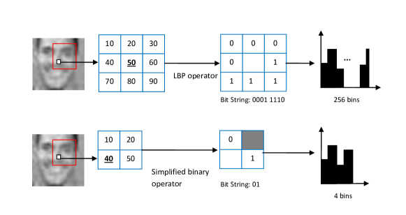
Figure 1: Top: An illustration of LBP. Bottom: An illustration of our edge binary pattern. Both descriptors have a radius of $1$ pixel.

II-C Joint Rectangular Features

In our work, we use the AdaBoost classifier with multidimensional decision stumps as weak learner. One disadvantage of training a weak learner with a single feature is that the generalization performance hardly improves in later rounds of boosting. Many researchers have observed that adding more weak learners can reduce the training error but not the generalization error [3, 10, 11]. More importantly, the detection performance of single features drops drastically in later stages of the cascade. We believe that single features are not discriminative enough to separate faces from difficult non-faces.

The use of feature co-occurrences in each weak classifier has been shown to yield higher classification performance compared to the use of a single feature [11]. Similar to Mita et al. [11], we solve this problem by applying the concept of joint features to create a more distinctive co-occurrence of features. Instead of using class-conditional joint probabilities, we approach this problem by using sparse least square regression to train our weak classifiers. Least square regression is proved to be one of the most effective weak classifiers in various literatures [12, 13]. Joint features using sparse least square regression make it possible to classify difficult samples that are misclassified by weak classifiers using a single feature.

Let training data sets consist of $n$ samples $(X_{i},y_{i})$, $i=1..n$, where $X_{i}=[R_{1},R_{2},..,R_{j}]$ is the vector of $1$D rectangular features and $y_{i}$ is an object class $\in\{-1,1\}$. The least square model has the form $f(X,\boldsymbol{\beta})=\beta_{1}R_{1}+\beta_{2}R_{2}+\cdots+\beta_{j}R_{j}+\beta_{0}$. The least square method finds optimum parameters, $\hat{\boldsymbol{\beta}}$, where the weighted sum of squared residuals, $\sum_{i=1}^{n}{w_{i}{[y_{i}-f(X_{i},\hat{\boldsymbol{\beta}})]}^{2}}$, is minimized. Here, $w_{i}$ is the sample weights. In order to construct a set of distinctive feature co-occurrences, we focus on a subset of rectangular features. In other words, we add a sparsity constraint into our least square problem. The optimization problem can now be defined as

$$\min_{i}\quad \sum_{i}{w_{i}{[y_{i}-f(X_{i},\hat{\boldsymbol{\beta}})]}^{2}},$$ (1)

$$\mathop{\mathrm{subject~{}to}}\nolimits\quad \operatorname{\bf Card}(\boldsymbol{\beta})=k,$$

where $\operatorname{\bf Card}(\boldsymbol{\beta})=k$ is an additional sparsity constraint and $\operatorname{\bf Card}(\cdot)$ counts the number of nonzero components. The problem is non-convex, combinatorial and NP-hard. Since, least square problem can be viewed as Generalized Rayleigh Quotient problem [14], an efficient greedy approach similar to the one proposed in [15] can be adopted here. In other words, the optimal solution to sparse generalized Eigen-value decomposition [15] is also the optimal solution to our sparse least square regression.

To improve the generalization performance, a simple decision stump is introduced to each rectangular feature. Hence, each feature value is represented by a decision stump’s output (binary response), specifying object or non-object, respectively. The threshold value in threshold function is selected based on AdaBoost sample weights in each iteration.

III Experiments

This section is organized as follows. The data sets used in this experiment, including how the performance is analyzed, are described. Experiments and the parameters used are then discussed. Finally, experimental results and analysis of different techniques are presented.

III-A Frontal Face Detection

Due to its efficiency, Haar-like rectangle features [1] have become a popular choice as image features in the context of face detection. We compare our rectangular features with Haar-like features. Similar to the work in [1], the weak learning algorithm known as decision stumps is used here due to their simplicity and efficiency.

III-A1 Performances on Single-node Classifiers

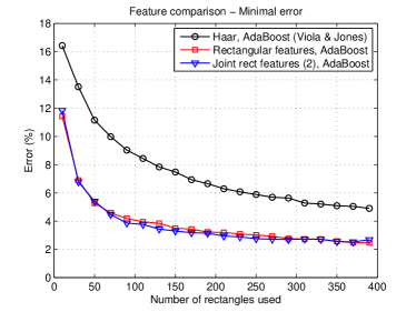
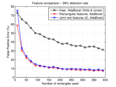
Figure 2: Best viewed in color. Comparison of (a) error rates between Haar-like features and rectangular features. The joint rectangular classifier consists of two rectangles in each weak classifier. (b) false alarm rates on test sets between Haar-like features and rectangular features.

In order to demonstrate the performance of our features, we replace Haar wavelet like features used in [1] with our features. In the first experiment, we compare a single strong classifier learned using AdaBoost with Haar wavelet like features and our proposed rectangular features. The data sets consist of $10,000$ mirrored faces. They were divided into three training sets and two test sets. Each training set contains $2,000$ face examples and $2,000$ non-face examples. The faces were cropped and rescaled to images of size $24\times 24$ pixels. For non-face examples, we randomly selected $5,000$ non-face patches from non-faces images and added $5,000$ difficult non-faces, for a total of $10,000$ patches. For each experiment, three different classifiers are generated, each by selecting two out of the three training sets and the remaining training set for validation. The performance is measured by two different curves:- the test error rate and the classifier learning goal (the false alarm error rate on test sets given that the detection rate on the validation set is fixed at $99\%$).

Experimental results are shown in Figs. 2 and 2. The following observations can be made from these curves. Having the same number of learned features, rectangular features achieves lower generalization error rate and false positive error than Haar features. Based on our observations, Haar features seem to perform slightly better than rectangular when the number of features is less than $5$. This is not surprising since Haar features contain more variety of shapes than our rectangular features. The first few selected Haar features often combine different parts of the faces and therefore would be more discriminative than our rectangular shape. The performance of our joint rectangular features is also shown in the figure. On face data sets, we observe a lower error rate when we combine two rectangular features. Combining three or more rectangular features does not improve the performance any further.

III-A2 Performances on Cascades of Strong Classifiers

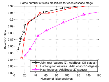
Figure 3: Performance comparison between our rectangular features, joint rectangular features and Haar features on cascades of strong classifiers.

In the next experiment, we used $2,500$ frontal faces ($5,000$ mirrored faces) that we obtained from [1]. All faces were cropped and rescaled to a size of $24\times 24$ pixels. For non-face examples, we randomly downloaded over $7,000$ images of various sizes from the internet. We used MIT+CMU test sets to test our system. The set contains $130$ images with $507$ frontal view faces. We set the scaling factor to $1.2$ and window shifting step to $1$. The technique used for merging overlapping windows is similar to [1]. Multiple detections of the same face in an image are considered false detections.

For fair evaluation of both rectangular and Haar-like features, we adopted a simple cascade as proposed in [1]. Each cascade layer consists of the same number of features (weak classifiers). The non-face samples used in each cascade layer are collected from false positives of the previous stages of the cascade (bootstrapping). The cascade training algorithm terminates when there are not enough negative samples to bootstrap. Fig. 3 shows a comparison between the Receiver Operating Characteristic (ROC) curves produced by both features. The ROC curves show that rectangular features outperform Haar-like features at all false positive rates. Similar to previous experiment, the combination of two rectangular features in each weak classifier performs best. From the figure, the performance gap between single and joint features is wider at low number of false positives, i.e., at $85\%$ detection rate, joint features achieve $10$ less false positives than single features. Experimental results indicate that the type of features we use has a crucial role in the ability of the system to generalize. Fig. 4 shows single and joint rectangular features selected in the first cascade layer. Most selected patches cover the area around the eyes and forehead.

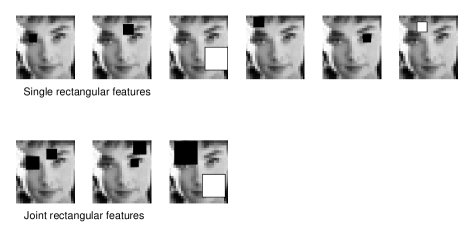
Figure 4: The first few selected rectangular features from the first layer of cascade. Black boxes indicate HOG features and white boxes indicate LBP feature.

Since, face labeling process is rather tedious and time consuming; it is quite common that the labeled faces are misaligned and rotated. In the next experiment, we compare the performance of rectangular features and Haar-like features on noisy face data sets. In other words, we want to determine how much effect the noisy training data will have on the detection performance. We automatically rotate, shift and illuminate faces in the training sets using some predefined rules. Some of the modified faces are shown in Fig. 5. Similar to previous experiments, we used AdaBoost to train both features. Some readers might point out that AdaBoost is vulnerable to handling noisy data and the use of other classifiers, e.g., LogitBoost [16] and BrownBoost [17], would yield better generalization. However, this would defeat the purpose of comparing Haar features with rectangular features. Table I shows detection rates of both features when trained on different noisy data sets and tested on MIT+CMU test sets. Based on our results, rectangular features are much better at handling noisy training data. We notice less performance drop when the classifier is trained with rectangular features.

The disadvantage of rectangular features compared to Haar-like features is that we now have to keep $8$ integral images in the memory for fast feature extraction (signed and unsigned vertical edge responses, signed and unsigned horizontal edge responses and $4$ bins for LBP histogram). In terms of an evaluation time, rectangular features have a higher evaluation time than Haar-like features due to an overhead in integral images’ calculation.

Figure 5: Manipulated faces. Top row: faces are exposed to random illumination changes and translated randomly. Second row: faces are randomly in plane rotated and exposed to random illumination changes. Third row: faces are randomly in plane rotated and randomly translated. Last row: faces are randomly rotated, randomly translated and exposed to random illumination changes.

TABLE I: Performance comparison of classifiers using rectangular features and Haar-like features on noisy data sets. Here, we compare the detection rate on MIT+CMU test sets when the number of false positives is $50$. R means faces are in plane rotated. L means faces are exposed to illumination changes (lighting). M means faces are translated by a few pixels (misaligned).

	Rectangle shaped	Haar-like features	Perf. Improvement
Original	$0.905$	$0.878$	$3.0\%$
R+L	$0.844$	$0.790$	$6.3\%$
M+L	$0.856$	$0.821$	$4.3\%$
R+M	$0.835$	$0.814$	$2.5\%$
R+M+L	$0.826$	$0.739$	$12.0\%$
Average	$0.853$	$0.808$	$5.5\%$

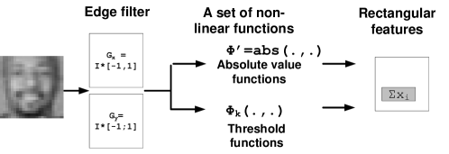
Figure 6: An illustration of rectangular features.

IV Discussion

In this paper, we proposed a simple and robust local feature descriptor for face detection. Our rectangular features can be denoted by a $4$-tuple, $(x,y,w,h)$, where $x$ and $y$ denote the $x$-coordinate and $y$-coordinate of the top left position of the block, $w$ and $h$ are the width and height of the rectangles, respectively. Rectangular features are based on simplified HOG and LBP features. Our simplified HOG can be viewed as a sum of edge responses, in vertical and horizontal directions. For unsigned gradients, we apply an absolute value function to edge responses. The absolute value of a real number is its numerical value without its sign. From image processing point of view, the absolute values of the intensity changes represent the magnitude of the edges without taking into consideration the polarity of the edges. Each rectangle is represented by a $4$-D feature vector, which is normalized to an $\ell_{2}$ unit length. Simplified binary operator can be viewed as applying the simple threshold function to both vertical and horizontal edge responses. The threshold function can be classified as one form of activation functions commonly used in neural network. The output of the functions takes on the value of $1$ or $0$ depending on the sign of both horizontal and vertical gradients, (2).

$$\phi_{1}(x,y)=\left\{\begin{array}[]{ll}1&\mbox{if $x\geq 0$ and $y\geq 0$};\\ 0&\mbox{otherwise},\end{array}\right.$$

$$\phi_{2}(x,y)=\left\{\begin{array}[]{ll}1&\mbox{if $x\geq 0$ and $y<0$};\\ 0&\mbox{otherwise},\end{array}\right.$$

$$\phi_{3}(x,y)=\left\{\begin{array}[]{ll}1&\mbox{if $x<0$ and $y\geq 0$};\\ 0&\mbox{otherwise},\end{array}\right.$$

$$\phi_{4}(x,y)=\left\{\begin{array}[]{ll}1&\mbox{if $x<0$ and $y<0$};\\ 0&\mbox{otherwise}.\end{array}\right.$$ (2)

where $x$ and $y$ denote vertical and horizontal edge responses.

An illustration of our rectangular features based on HOG and LBP is shown in Fig. 6. We can generalize rectangular features as follows. First, we apply edge filters to the original image. Edge filter is one of the most popular techniques used to detect a rate of changes at any given pixel coordinates. Edge responses can be calculated from partial derivatives in horizontal and vertical directions of a given pixel location. After deriving vertical and horizontal edge responses, we apply two non-linear functions to these responses; namely absolute value function and $2$-D threshold function. By introducing non-linearity into low-level features, we observe an improvement in the overall performance on visual classification tasks. These non-linear functions might look over-simple. However, many researchers have reported that applying these simple approach often leads to performance improvement in vision applications, e.g., binary operator has been used in LBP to describe image texture as described in Section II-A, absolute value function has also been used in Speeded Up Robust Features (SURF) [18] where it performs remarkably well in describing key-point descriptor. In summary, our rectangular features consider the change of pixel intensities in a small image neighborhood to provide an approximate representation of edge responses inside the specific region. This finding raises several open questions related to possible face detection features. In the future we plan to research on learning a more efficient rectangular feature, which would be more memory efficient, work well on general objects and can achieve a comparable speed to Haar-like features.

V Conclusion

In this work, we proposed the use of simple edge descriptors, which combine the discriminative power of HOG with the strength of LBP operators. Since, single feature is not discriminative enough to separate faces from difficult non-faces, we further improve the generalization performance of our simple features by applying feature co-occurrences. Experimental results show that our new features not only outperform Haar-like features but also yield better generalization when training on noisy data. On average, we achieve a performance improvement of $5.5\%$ when trained with rectangular features.

References

- [1] P. Viola and M. J. Jones, “Robust real-time face detection,” Int. J. Comp. Vis., vol. 57, no. 2, pp. 137–154, 2004.
- [2] R. Lienhart and J. Maydt, “An extended set of haar-like features for rapid object detection,” in Proc. IEEE Int. Conf. Image Process., vol. 1, 2002, pp. 900–903.
- [3] S. Z. Li and Z. Zhang, “Floatboost learning and statistical face detection,” IEEE Trans. Pattern Anal. Mach. Intell., vol. 26, no. 9, pp. 1112–1123, 2004.
- [4] C. Huang, H. Ai, Y. Li, and S. Lao, “High-performance rotation invariant multiview face detection,” IEEE Trans. Pattern Anal. Mach. Intell., vol. 29, no. 4, pp. 671–686, 2007.
- [5] K. Levi and Y. Weiss, “Learning object detection from a small number of examples: The importance of good features,” in Proc. IEEE Conf. Comp. Vis. Patt. Recogn., vol. 2, Washington, DC, 2004.
- [6] N. Dalal and B. Triggs, “Histograms of oriented gradients for human detection,” in Proc. IEEE Conf. Comp. Vis. Patt. Recogn., vol. 1, San Diego, CA, 2005, pp. 886–893.
- [7] T. Ojala, M. Pietik inen, and T. M enp , “Multiresolution gray scale and rotation invariant texture analysis with local binary patterns,” IEEE Trans. Pattern Anal. Mach. Intell., vol. 24, no. 7, pp. 971–987, 2002.
- [8] X. Wang, T. X. Han, and S. Yan, “An hog-lbp human detector with partial occlusion handling,” in Proc. IEEE Int. Conf. Comp. Vis., 2009.
- [9] D. G. Lowe, “Distinctive image features from scale-invariant keypoints,” Int. J. Comp. Vis., vol. 60, no. 2, pp. 91–110, 2004.
- [10] J. Wu, S. C. Brubaker, M. D. Mullin, and J. M. Rehg, “Fast asymmetric learning for cascade face detection,” IEEE Trans. Pattern Anal. Mach. Intell., vol. 30, no. 3, pp. 369–382, 2008.
- [11] T. Mita, T. Kaneko, B. Stenger, and O. Hori, “Discriminative feature co-occurrence selection for object detection,” IEEE Trans. Pattern Anal. Mach. Intell., vol. 30, no. 7, pp. 1257–1269, 2008.
- [12] S. Avidan, “Ensemble tracking,” IEEE Trans. Pattern Anal. Mach. Intell., vol. 29, no. 2, pp. 261–271, 2007.
- [13] T. Parag, F. Porikli, and A. Elgammal, “Boosting adaptive linear weak classifiers for online learning and tracking,” in Proc. IEEE Conf. Comp. Vis. Patt. Recogn., Anchorage, 2008, pp. 1–8.
- [14] B. Moghaddam, A. Gruber, Y. Weiss, and S. Avidan, “Sparse regression as a sparse eigenvalue problem,” in Information Theory and Applications Workshop, 2008, pp. 219–225.
- [15] B. Moghaddam, Y. Weiss, and S. Avidan, “Fast pixel/part selection with sparse eigenvectors,” in Proc. IEEE Int. Conf. Comp. Vis., 2007, pp. 1–8.
- [16] J. Friedman, T. Hastie, and R. Tibshirani, “Additive logistic regression: a statistical view of boosting,” Ann. Statist., vol. 28, no. 2, pp. 337–407, 2000.
- [17] Y. Freund, “An adaptive version of the boost by majority algorithm,” Mach. Learn., vol. 43, no. 3, pp. 293–318, 2004.
- [18] H. Bay, A. Ess, T. Tuytelaars, and L. V. Gool, “Speeded-up robust features (surf),” Comp. Vis. Image Understanding, vol. 110, no. 3, pp. 346–359, 2008.