Use of multiple singular value decompositions to analyze complex intracellular calcium ion signals

Abstract

We compare calcium ion signaling ($\mathrm{Ca}^{2+}$) between two exposures; the data are present as movies, or, more prosaically, time series of images. This paper describes novel uses of singular value decompositions (SVD) and weighted versions of them (WSVD) to extract the signals from such movies, in a way that is semi-automatic and tuned closely to the actual data and their many complexities. These complexities include the following. First, the images themselves are of no interest: all interest focuses on the behavior of individual cells across time, and thus, the cells need to be segmented in an automated manner. Second, the cells themselves have 100$+$ pixels, so that they form 100$+$ curves measured over time, so that data compression is required to extract the features of these curves. Third, some of the pixels in some of the cells are subject to image saturation due to bit depth limits, and this saturation needs to be accounted for if one is to normalize the images in a reasonably unbiased manner. Finally, the $\mathrm{Ca}^{2+}$ signals have oscillations or waves that vary with time and these signals need to be extracted. Thus, our aim is to show how to use multiple weighted and standard singular value decompositions to detect, extract and clarify the $\mathrm{Ca}^{2+}$ signals. Our signal extraction methods then lead to simple although finely focused statistical methods to compare $\mathrm{Ca}^{2+}$ signals across experimental conditions.

, , , and

t1Supported by a postdoctoral training grant from the National Cancer Institute (CA90301). t2Supported by a grant from the National Cancer Institute (CA57030) and by Award Number KUS-CI-016-04, made by King Abdullah University of Science and Technology (KAUST). t3Supported by a grant from the National Science Foundation (DMS-06-06580). t4Calcium imaging performed in the College of Veterinary Medicine & Biomedical Sciences Image Analysis Laboratory, was supported by NIH-NIEHS Grants P30-ES09106, P42-ES04917 and T32 ES07273.

1 Introduction

Scientifically, this paper is about the study of the effects of 2,3,7,8-Tetrachlorodibenzo-p-dioxin (TCDD) on calcium ion signaling ($\mathrm{Ca}^{2+}$) in myometrial cells. The importance of $\mathrm{Ca}^{2+}$ signaling in cell function, for example, metabolism, contraction, cell death, communication, cell proliferation, has been studied in numerous types of cells; see Putney (1998). TCDD itself is a toxicant by-product of incomplete combustion of fossil fuels, woods and wastes and is known to adversely effect reproduction, development and the immune system as well as being a probable carcinogen.

The essential feature of these data is that they present themselves as movies of 512 images, or time series of images after oxytocin exposure. To best appreciate the complexity of the data, and thus this paper, readers should first look at two of the movies, in the Supplementary Materials, one without and one with TCDD exposure.

The experiment leading to these images is described in detail in Section 2. However, the movies show that the data are complex, and analysis of them is not simple. This paper describes novel uses of singular value decompositions (SVD) and weighted versions of them (WSVD) to extract the signals from such movies, in a way that is semi-automatic and tuned closely to the actual data and their many complexities. Here we describe a few of these complexities:

1. []

2. The data consist of 512 images. Myometrial cells can be seen in these images, which start out in their native state and are then exposed to an oxytocin stimulus, at which point $\mathrm{Ca}^{2+}$ expression becomes pronounced. The cells themselves are fixed to a substrate and do not move over time.

3. The images themselves are of no intrinsic interest: what matters is how the individual cells express $\mathrm{Ca}^{2+}$. This means that segmenting the image to obtain the cells is a crucial first step. To see what has been done in the past, consider Figure 1, which gives a sequence of images in the first 2 minutes of the experiment. Because it is difficult to distinguish cell boundaries before oxytocin is delivered, it is common to use a static approach. Specifically, the brightest image is used to isolate the cells, with cell boundaries drawn by hand. This technique, although practical, is not semi-automatic and uses only a small fraction of the information available because it ignores the 511 other images that could have pertinent information about the cell boundary. This could potentially lead to under or overestimation of the cell boundaries. Instead, we will describe a method that allows use of all 512 images in order to determine cell location. Our approach utilizes the brightest image to get a rough idea of the cell location and then obtains a summary of the resulting pixel-wise matrix of all 512 images to refine the cell boundaries.

   

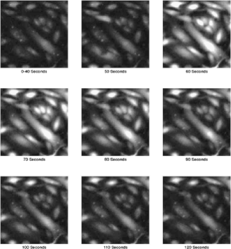
   Figure 1: Oxytocin-induced calcium response in myometrial cells during the first 2 minutes of the experiment. Cells were cultured in a low level of estrogen/progesterone and were treated with 10 nM TCDD for 24 hours. Cells were then loaded with the Fluo-4, washed and then stimulated with 20 nM oxytocin following identification of basal calcium levels in cells. The movie of this cell line as well as the nontreated one cultured in low hormone level are available as part of the Supplementary Materials.

4. Each segmented cell will contain 100$+$ pixels, and each of these pixels is its own movie or curve. Immediately, one is faced with the problem of summarizing these curves. The usual choice of a summary statistic in $\mathrm{Ca}^{2+}$ signal publications is the normalized average signal across time, where “normalized” means that the whole signal is divided by the initial signal values recorded before the stimulus is delivered to the cells; see Barhoumi et al. (2002) and Burghardt et al. (1999). Hence, signal amplitude is measured in units of “fold change,” compared to the $\mathrm{Ca}^{2+}$ signal before stimulus. While convenient, this method ignores the potential for additional information in the wealth of pixel information, information we aim to extract, and it is in addition not necessarily the best way to normalize the data.

5. Having extracted the basic signal, we face a further obstacle. An unusual feature of these data is that some of the pixels in most of the cells reach image saturation. This type of image censoring has the potential to distort downstream statistical analysis, is generally ignored in the literature, and needs to be accounted for. That is, we wish to clarify the original signal to account for image saturation.

6. Having segmented the cells, and extracted and clarified the cell $\mathrm{Ca}^{2+}$ signal, we are then in a position to understand some of the effects of TCDD exposure.

7. The main point of this paper is to extract the information in the movies, in a semi-automatic way that reduces the potential for bias.

8. In this paper we will show how to use the singular value decomposition (SVD) and a novel weighted singular value decomposition (WSVD) to perform the four crucial steps I–IV. Each step requires a different use of the SVD or WSVD. We demonstrate that novel uses of SVD/WSVD help us understand the effect of TCDD exposure.

Our paper is organized in the following manner. In Section 2 we describe the experiment and the data. We proceed to restate the singular value decomposition (SVD) in Section 3 and demonstrate how to use it to obtain the EigenPixel and EigenSignal vectors. In Section 4 we outline the use of the SVD to detect the $\mathrm{Ca}^{2+}$ signal from images, that is, to segment the cells. In Section 5 we use yet another SVD to isolate the $\mathrm{Ca}^{2+}$ signal from the resulting pixel-wise matrices. We implement a weighted SVD, WSVD, with a clever choice of weights in Section 6, and use it to remove the saturation effect on the $\mathrm{Ca}^{2+}$ signal. Finally, in Section 7 we compare the control and treated cells by applying the SVD once more to obtain one point summary values for each cell, that is, EigenCells, which enable us to distinguish between control and treated groups. We offer some concluding remarks in Section 8.

2 Experiment

2.1 Introduction

The essential statistical details of this experiment are that there are myometrial cells fixed to different substrates, one of which is exposed to TCDD and the other of which is not. Shortly after image capturing commences, the cells are exposed to oxytocin, thus stimulating the $\mathrm{Ca}^{2+}$ signal. The main goal is to compare the TCDD exposure to the control. What follows are some of the details of the experiment.

2.2 Treatments

Myometrial cells, which comprise the contractile middle layer of the uterine wall, were cultured in three levels of an estrogen/progesterone hormone combination: basal, low and high. The “basal” level is the one in which the cells were cultured, the “low” level of hormone is slightly higher than that found in women before pregnancy and the “high” level is the level of a pregnant woman at full term. Our work presents data from two different treatments (control or TCDD) with 3 different levels of hormones in the culture medium (basal, low and high).

The treated cells received a 100 nM solution of TCDD 24 hours before the experiment. Cells are cultured on coverglass chambered slides. All cells were then washed and loaded with 3 µM Fluo-4 for 1 hour at $\mathrm{37^{\circ}C}$: fluorescent probe Fluo-4 is one of many dyes used to detect changes in $\mathrm{Ca}^{2+}$ within cells. Fluo-4 is typically excited by visible light of about 488 nM, and emits about 100 fold greater fluorescence at about 520 nM upon binding free $\mathrm{Ca}^{2+}$. Following loading, cells were washed and placed on the stage of the confocal microscope. Cells were then scanned five times to establish the basal level of $\mathrm{Ca}^{2+}$ prior to addition of 20 nM oxytocin, the hormone used in this study to stimulate $\mathrm{Ca}^{2+}$ signal in these cells. Scanning continues at 10 second intervals for approximately 85 minutes, leading to 512 images (100 $\times$ 100 pixels) containing 20–50 cells per treatment.

2.3 Imaging

The data captured in these experiments are digital images of $\mathrm{Ca}^{2+}$ fluorescence of individual cells. The bit depth of images used in this study is of 8 bits, which translates to $2^{8}$ or 256 possible grayscale values in the image. Unfortunately, it often happens that the maximum concentrations detected in these images are limited by the bit depth. This may sometimes result in saturation and lead to underestimation of changes in $\mathrm{Ca}^{2+}$ signals, especially when multiple treatments are performed and accurate evaluation of these differences is required.

Figure 1 shows a response to the oxytocin stimulus, in cells treated with TCDD and cultured in a low estrogen/progesterone hormone level. The maximal reaction due to the oxytocin challenge appears at 60 seconds and then the cells return to their steady state. Notice that not all cells go back to their steady state at the same rate. In fact, there is residual fluorescence in some cells at the top of each of the images in Figure 1, long after the initial peak of fluorescence at 60 seconds.

2.4 Overview of what is to come

In order to study the intracellular $\mathrm{Ca}^{2+}$ signal, we make use of the singular value decomposition in four ways. First we isolate or (a) detect the cell itself. To do this we perform a singular value decomposition on a matrix made up of pixels from a rough segmentation of each cell. The spatial plot of the first EigenPixel resulting from this SVD is used to determine which pixels are important when harnessing the signal. The next step is to (b) extract the $\mathrm{Ca}^{2+}$ signal. In this step we apply the SVD on the resulting pixel-wise matrix from the previous step and obtain the first EigenSignal, which contains most of the $\mathrm{Ca}^{2+}$ signal information of the cell of interest. The third step is to (c) clarify that signal. In this step we adapt the usual SVD and introduce a weighted SVD which takes care of two problems: (1) it imputes values where pixel saturation occurs and (2) it weights the influence of each pixel based on variance. Finally, the last step in our study of intracellular $\mathrm{Ca}^{2+}$ signal is to (d) compare the effect of the carcinogen TCDD across experimental conditions to see how it affects the $\mathrm{Ca}^{2+}$ response. To accomplish this, we use the SVD again to obtain one point summary values for each cell.

3 SVD after rough segmentation

3.1 Outline

This section describes the well known SVD and outlines part of how we will use it, after large rectangular regions containing each cell have been obtained (rough segmentations). We particularly need to describe some terminology for future use.

3.2 EigenPixels and EigenSignals

The singular value decomposition (SVD) is a widely used matrix factorization technique. For example, the SVD was used to analyze microarray expression data, where the rows of the matrix in question comprise the genes and the columns represent the expression arrays [Alter et al. (2000)]. This use of the SVD introduced the idea of transforming the gene, array space to an “eigengene,” “eigenarray” space that is reduced and diagonalized. We will draw inspiration from this approach and show that we can use “eigen $\mathrm{Ca}^{2+}$ signal” or EigenSignal vectors to summarize the $\mathrm{Ca}^{2+}$ response for each cell in the experiment and we will later describe how we acquired matrix representations for each cell.

We first describe how to obtain “eigen pixel” and “eigen $\mathrm{Ca}^{2+}$ signal” vectors, using the SVD. To accomplish this, we will present the singular value decomposition in the context of our data, assuming that a rough segmentation of the cells has been performed. For all treatments considered in this work, we represent each cell as a matrix of $\mathrm{Ca}^{2+}$ intensity, in grayscale values, that has a number of pixels which comprise the cell, for all 85 minutes of the experiment. Each matrix has $n$ rows and $m$ columns, where $n$ is the number of pixels that represent the cell and $m$ is the number of time points in the experiment. All cells were observed the same number of times so $m=512$. Let $X_{k}$ represent the $n\times m$ calcium signal matrix for the $k$th-cell. The singular value decomposition of $X_{k}$ is

$$X_{k}=U_{k}S_{k}V_{k}^{\mathrm{T}}.$$ (1)

Here $V_{k}$ is an $m\times n$ matrix whose column vectors, $\mathbf{v}_{kj}\in\mathbb{R}^{m}$, form an orthonormal basis for the $\mathrm{Ca}^{2+}$ signal, and are called EigenSignal vectors. In (1) $U_{k}$ is an $n\times n$ matrix whose column vectors, $\mathrm{u}_{kj}\in\mathbb{R}^{n}$, form an orthonormal basis for the pixels of the cell, called EigenPixel vectors. In addition, $S_{k}$ is an $n\times n$ square matrix of singular values arranged from largest to smallest $s_{k1}\geq s_{k2}\geq\cdots\geq s_{kn}$.

We can generate a rank-$L$ matrix that approximates $X_{k}$ by using the first $L$ $u_{kj}$ and $v_{kj}$ vectors, that is,

$$X_{k}^{L}=\sum_{j=1}^{L}u_{kj}s_{kj}v_{kj}^{\mathrm{T}}.$$ (2)

In equation (2) $X_{k}^{L}$ is the best rank-$L$ matrix that approximates $X_{k}$, in the sense that it minimizes the sum of squares difference between $X_{k}^{L}$ and $X_{k}$ among all rank-$L$ matrices [Trefethen and Bau (1997)]. Low rank approximations are useful because less data are needed to represent the original matrix; these techniques are often used in image compression. We will use the smallest number of EigenPixel and EigenSignal vectors that summarize both pixel and $\mathrm{Ca}^{2+}$ signal information.

4 $\mathrm{Ca}^{2+}$ cell segmentation

4.1 Peak image

The cells used in this study are cultured as monolayer on coverglass chambered slides. This allows easy imaging of the cells over time without any movement: the cells in this study are fixed in a substrate. This fact is essential to the work that follows.

As may be apparent from the sequence of images shown in Figure 1, it is difficult to distinguish cell boundaries before oxytocin is delivered. For this reason, in order to determine the location of the cells, as well as their boundaries, it is common to use the brightest image to isolate the cells. This technique, although practical, only uses a small fraction of the information available because it ignores the 511 other images that could have pertinent information about the cell boundary. Instead, we propose that a summary of these 512 images should be used to determine cell location. Our approach makes use of the brightest image, or “peak” image, to get a rough idea of the cell location and then uses a summary of the resulting pixel-wise matrix of all 512 images to refine the cell boundary that will be used for the rest of the analysis. We use the image where we see the most distinction between cell boundaries as the “peak” image.

Figure 2: The initial rough rectangular segmentation of cell 2 from the treated group of low hormone level and the corresponding 777 $\times$ 512 pixel-wise matrix for this rectangular region.

4.2 $\mathrm{Ca}^{2+}$ signal detection via first eigenpixel

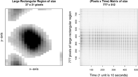
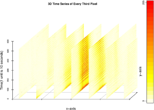
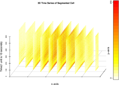
Once the “peak” image from each cell line is identified, we draw very large rectangular regions each containing a cell. Each rectangular region assures that the boundaries of the cell of interest are contained within it, although there may be parts of other cells that fall in this rectangular region. Figure 2 shows the rectangular region chosen from the “peak” image to represent the rough segmentation of cell 2, from the treated group in the low hormone level. Figure 2 also displays the resulting 777 $\times$ 512 pixel-wise matrix derived by taking the 777 pixels that represent the rectangular region from each distinct image at every one of the 512 time points. The right panel of Figure 2 does not respect the spatial location of the pixels. A better view of how the 3-dimensional time series of $\mathrm{Ca}^{2+}$ intensity evolves is shown in Figure 3. This perspective plot of every third pixel in the rough segmentation shows the spatial location of pixels over time. Notice that the oscillations in the signal concentrate in the center of the $x$–$y$ plane and evolve over time in the $z$-axis.

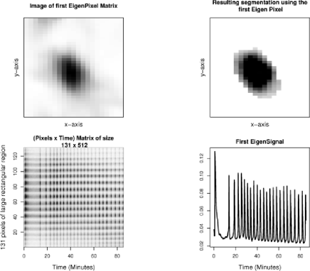
If $X_{2}$ represents the 777 $\times$ 512 pixel-wise matrix of pixels $\times$ time for cell 2, shown in the right panel of Figure 2, then we obtain a summary of the pixel information by taking the SVD of $X_{2}$ and obtaining the first EigenPixel. As explained in Section 5.2 below, only the first singular value explains the majority of the variance in these data, hence, the first EigenPixel summarizes all the pixel information to one vector of size 777. We take this vector and plot it spatially on the corresponding pixel location. What we get is a 2-dimensional image where the pixel intensity reflects the importance of the pixel in representing the $\mathrm{Ca}^{2+}$ signal of this cell (top left panel of Figure 4). This image is a better candidate for use in identification of the $\mathrm{Ca}^{2+}$ signal than the “peak” image because it summarizes the importance of each pixel across the 512 images in the experiment. This is our first use of the SVD and the way in which we will detect the $\mathrm{Ca}^{2+}$ signal for all cells in this experiment.

Figure 3: 3D plot of the $\mathrm{Ca}^{2+}$ intensity in the rough segmented region of cell 2 from the treated group of low hormone level, corresponding to the left panel of Figure 2. The $x$–$y$ coordinates correspond to space and the vertical coordinate to time. Every fourth pixel is shown.

Figure 4: Top row: Image of the first EigenPixel vector obtained from the SVD of the rough 777 $\times$ 512 pixel-wise matrix and the resulting segmentation of cell 2 after using the first EigenPixel to perform the segmentation. Bottom row: The corresponding 131 $\times$ 512 pixel-wise matrix for this new segmentation and the corresponding first EigenSignal over the 85 minute experiment.

Figure 5: 3D plot of the $\mathrm{Ca}^{2+}$ intensity for the final segmentation of cell 2 from the treated group of low hormone level, corresponding to the left panel of Figure 4. The x–y coordinates correspond to space and the vertical coordinate to time. Every fourth pixel is shown.

4.3 $\mathrm{Ca}^{2+}$ final segmentation

Once we obtain this first EigenPixel image from $X_{2}$, we use the EBImage package from Bioconductor to segment and index the cell [R Development Core Team (2008)]. We first blurred the image to smooth out any noisy pixels. We then used thresholding to pick out the region of high pixel values which usually contains the cell, and finally used a watershedding algorithm to close the cell boundaries and separate other cell chunks that are close together. The result is the final segmentation of the cell shown in the top right panel of Figure 4. Notice that all we have done is pick the region with highest EigenPixel intensity which in turn should give us the spatial location of the pixels that contain most of the $\mathrm{Ca}^{2+}$ signal information. We then collect each of the 131 pixels in this final segmentation from each of the 512 images and get a matrix representation of the cell; see the bottom left panel of Figure 4. As before, this matrix does not respect the spatial location of the pixels, hence, we provide a 3-dimensional plot where each of the pixels in the final segmentation is displayed over time; see Figure 5. It is easier to appreciate the spatial pattern of the $\mathrm{Ca}^{2+}$ signal and where it concentrates on the $x$–$y$ plane at any time.

We used this segmentation process to generate contours of each cell, and used these contours to pick out the cell position from every image at every one of the 512 time points. This process yielded 20–50 cells from each treatment.

The oscillatory behavior observed in Figures 4 and 5 and throughout the text are present because calcium ions ($\mathrm{Ca}^{2+}$) are responsible for many important physiological functions. In smooth muscle cells that surround hollow organs of the body, transient increases in intracellular $\mathrm{Ca}^{2+}$ can be stimulated by a number of hormones to activate smooth muscle contraction. Because sustained elevation of $\mathrm{Ca}^{2+}$ is toxic to cells, $\mathrm{Ca}^{2+}$ signals in many cell types frequently occur as repetitive increases in $\mathrm{Ca}^{2+}$, referred to as $\mathrm{Ca}^{2+}$ oscillations. The periodic $\mathrm{Ca}^{2+}$ spikes which increase with increasing hormone concentration are thought to constitute a frequency encoded signal with a high signal-to-noise ratio which limits prolonged exposure of cells to high intracellular $\mathrm{Ca}^{2+}$; see Sneyd, Keizer and Sanderson (1995). Interestingly, the frequency of $\mathrm{Ca}^{2+}$ oscillations in smooth muscle cells is relatively low (e.g., 2–10 MHz) [see Burghardt et al. (1999)], whereas in liver cells which use $\mathrm{Ca}^{2+}$ oscillations to stimulate ATP production in mitochondria and the breakdown of glycogen to glucose, the frequency of $\mathrm{Ca}^{2+}$ oscillations is much greater (e.g., range from 5 to 100 MHz); see Barhoumi et al. (2002). The spatial and temporal organization and the control of these intracellular $\mathrm{Ca}^{2+}$ signals is of considerable interest to cellular biologists.

5 Signal extraction

5.1 Overview

The top right panel of Figure 4 shows the region that represents cell 2 and the bottom left panel shows the resulting 131 $\times$ 512 pixel-wise matrix for the final segmentation, which we will label as $X^{\prime}_{2}$. We then use the singular value decomposition once again and obtain the first EigenSignal from the $X^{\prime}_{2}$ matrix shown in the bottom right panel of Figure 4; this is our $\mathrm{Ca}^{2+}$ signal extraction step. The $\mathrm{Ca}^{2+}$ signal produced from this step is a candidate signal that represents a summary of the $\mathrm{Ca}^{2+}$ intensity for the cell in question.

5.2 First EigenPixel and EigenSignal

When we take the SVD of each matrix for each cell, in all cell lines, we find that the first EigenSignal vector is enough to give a good representation of the $\mathrm{Ca}^{2+}$ signal in these data, because the first singular value basically dominates the signal in the data. In fact, if we take the ratio of first to second singular values for each cell and take the mean, we find that on average the first singular value is between 8 to 10 times larger than the second, and many times larger than the $3$rd and $4$th singular values. The left panel of Figure 6 shows the variance explained by the first five singular values of the SVD of cell 11 in the control group of the high hormone level cell line, where the first component explains 97% of the variance. On average, the variance explained by the first component in each of the 187 cells considered across all cell lines in this experiment is 97%. The right panel of Figure 6 shows the distribution of the variance explained by the first component for each of the 187 cells. The minimum variance explained by the first singular value among the 187 cells is 83%, hence the first EigenSignal and EigenPixel vectors that correspond to this first singular value summarize almost all the $\mathrm{Ca}^{2+}$ signal and pixel information in each of these matrices. For this reason we will assume that only the first EigenSignal and first EigenPixel are needed to summarize the $\mathrm{Ca}^{2+}$ signal and pixel information in the data.

Figure 6: Left: Variance explained by the first 5 components in the SVD of the pixel-wise matrix that represents one cell (11) from the control group in the high hormone treatment. Right: Variance explained by the first component in the SVD in each of the 187 cells examined in all six treatments used in the study.

6 $\mathrm{Ca}^{2+}$ signal clarification and cell saturation

6.1 The problem of saturation

The saturation phenomenon is based upon the fluorescence detection system. The fluorescence detection system utilized in experiments presented in this report is a photomultiplier detector tube (PMT). This detector does not count individual photons; rather it requires a certain minimum number of photons to activate an electrode which will emit a small number of electrons which are subsequently amplified in a stepwise fashion. The readout of the PMT is on a 256 grey scale level. Occasionally the amplified signal can reach saturation if the fluorescence output of the calcium signal being detected is very high. Normally, the settings of the PMT are adjusted so as not to reach saturation, however, detection of the low end of the fluorescence signal is very important.

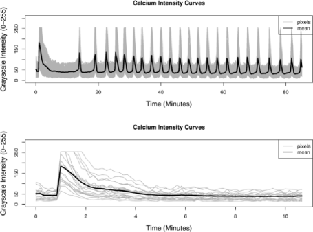
Notice that the grayscale values of some of the pixels that represent cell 2, shown in Figure 4, reach a ceiling of 255; see Figure 7. This is especially noticeable after the cell received the oxytocin stimulus around 1 minute into the experiment. Because the individual pixel values reflect the $\mathrm{Ca}^{2+}$ level in the cell, $\mathrm{Ca}^{2+}$ summary measures will undoubtedly be affected if the pixels reach the ceiling of 255. Also notice the variability in individual pixel values. The bottom panel of Figure 7 shows the intensity of 20 pixels over time and it is clear that some may reach maximum intensity values that are larger than 255 and some at much lower values. We do not model the behavior of individual pixels in this work but it can certainly be considered in the future.

Two questions are immediate. First, how is the EigenSignal affected when pixel values reach the saturation level of 255? Second, how should one process the $\mathrm{Ca}^{2+}$ signal once pixel saturation has been detected? We implement the algorithm introduced by Gabriel and Zamir (1979) and let the saturated pixels be missing data to address this issue. To our knowledge, there are no methods in the literature available to deal with the clarification of $\mathrm{Ca}^{2+}$ signal curves and our attempt is the first of its kind.

Figure 7: Top: The Calcium intensity curves over the 85 minute experiment of the 131 pixels in the $131\times 512$ pixel-wise matrix $X^{\prime}_{2}$. Bottom: 20 randomly selected pixels from $X^{\prime}_{2}$.

6.2 The weighted SVD

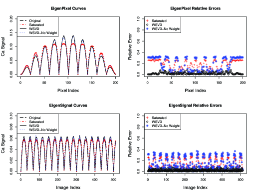
Although the first EigenSignal is a reasonable measure to use when summarizing the $\mathrm{Ca}^{2+}$ signals of the pixel-wise matrices, there are drawbacks if used without adjustment. If there are too many pixels that reach the saturation point, the signal can be under or over-estimated at different time points in the experiment and a misinterpretation of the signal amplitude can occur. It is intuitive to understand how the signal can be under-estimated due to saturation, but over-estimation of the summary signal is certainly an unexpected phenomenon which we will explain. Because pixels reach a saturation, the signal summary is undoubtedly affected by this lack of information on maximal values attained by such pixels. In the course of the time series where many pixels reach saturation, the signal is under-estimated around the peaks, but the effect of this under-estimation results in an over-estimation during a time where no pixels reached saturation. Figures 8 and 9 show this phenomenon. The over-estimation is due to the normalization requirement of the singular vectors and the right skewness of the cross-sectional intensity distribution.

To correct these over- and under-estimation effects, we must remove the effect of the saturated pixels and recalculate the $\mathrm{Ca}^{2+}$ signal without their influence. One approach is to simply remove every row of the pixel-wise data matrix which contains a saturated pixel and recompute the $\mathrm{Ca}^{2+}$ signal using the resulting matrix; however, this could lead to the removal of a significant number of rows from the data matrix. Instead, we propose to implement the weighted SVD, WSVD, using the low rank matrix approximation of Gabriel and Zamir (1979) where we introduce the use of indicators in the weights, as in Beckers and Rixen (2003), to treat the saturated pixels as missing data and use a clever choice of weights that allows for accurate recovery of the original signal.

It is important to note that our “missing data” is not really missing, we know that the saturated pixels must at least attain a value of 255. Hence, if we observe values that are below this threshold in our imputation, we would certainly know that we’ve made an error. We implement a check in our algorithm that gives us a flag if a value that is initially saturated falls below its saturation point.

Imputation of missing values in the SVD is not a new subject. As noted by Kurucz, Bencz$\acute{\mathrm{u}}$r and Csalog$\acute{\mathrm{a}}$ny (2007), it was first addressed in Ruhe (1974) and then refined by Gabriel and Zamir (1979). Recently, Liu et al. (2003) extended the work of Gabriel and Zamir (1979) to use outlier resistant regressions instead of simple least squares. Several new EM based imputation methods have been introduced. In particular, Troyanskaya et al. (2001) uses such a method to impute missing values into microarray experiments while using the SVD to obtain relevant eigen-genes and eigen-arrays. For further discussion on EM type estimators and a more complete review of the literature, see Kurucz, Bencz$\acute{\mathrm{u}}$r and Csalog$\acute{\mathrm{a}}$ny (2007).

Figure 8: Top row: Simulated data matrix (before adding noise) to be tested. Bottom row: First EigenSignal and EigenPixel curves obtained from the data matrix shown above.

Figure 9: Top row: EigenPixel vectors of the original, saturated, weighted SVD (WSVD) and WSVD with no weights (WSVD-No Weight) and the relative error of the saturated and final WSVD and WSVD-No Weight EigenPixels. Bottom row: EigenSignal vectors of the original, saturated, weighted SVD (WSVD) and WSVD with no weights (WSVD-No Weight) and the corresponding error curves of the saturated and final WSVD and WSVD-No Weight EigenSignals.

Although an EM type method could certainly be applied in this context, we choose to use the iterative algorithm of Gabriel and Zamir (1979) because of its speed in convergence and because we do not wish to make distributional assumptions about the data. Now, because the signal variance in our data follows the behavior of the signal itself, we opt to use a variance weight in the imputation scheme. Of course initialization of the algorithm is tricky, in particular, when $w_{ij}=0$, but our use of the first EigenPixel and EigenSignal to initialize the algorithm proves to work well; see Gabriel and Zamir (1979) for more discussion on initialization.

The premise of our approach is that each cell has a “true” $\mathrm{Ca}^{2+}$ signal and we are not able to observe that signal because there are only a finite number of pixel values available to capture it. The details of our implementation are provided below.

Let $\mathbf{u}$ and $\mathbf{v}$ be the first EigenPixel and EigenSignal associated with the second SVD used to extract the putative $\mathrm{Ca}^{2+}$ signal, which includes saturated pixels, so that $\mathbf{u}$ and $\mathbf{v}$ comprise most of the pixel and signal information of some cell. Continuing with the example from the previous section, the matrix of interest is $X^{\prime}_{2}$. Let the dimensions of the $X^{\prime}_{2}$ be $n\times m$; because most of the variation is explained by the first component in the SVD, the rank one approximation can be obtained by minimizing the error

$$\sum_{i=1}^{n}\sum_{j=1}^{m}(x^{\prime}_{2ij}-u_{i}v_{j})^{2}$$ (3)

with respect to $\mathbf{u}$ and $\mathbf{v}$. We also wish to weight each term in the double summation so that it removes the influence of saturated pixels and takes into account the appropriate variation. We let the weights be $w_{ij}=\mathrm{I}_{ij}/(u_{i}v_{j})^{2}$, where $\mathrm{I}_{ij}=0$ when $x^{\prime}_{2ij}=255$, that is, pixel is saturated, and $\mathrm{I}_{ij}=1$, otherwise. Beckers and Rixen (2003) proposed using an indicator to deal with missing data. We supplement this approach by using $(u_{i}v_{j})^{2}$ to scale the term in the summation of (3) so that the variance is no larger than 1. Now our new minimization problem becomes

$$\sum_{i=1}^{n}\sum_{j=1}^{m}w_{ij}(x^{\prime}_{2ij}-u_{i}v_{j})^{2}.$$ (4)

We solve the minimization by alternating between $u_{i}$ and $v_{j}$. Fixing $j$, we can expand the expression in (4), let $A_{j}(\mathbf{u})=\sum_{i}\mathrm{I}_{ij}(x^{\prime}_{2ij}/u_{i})^{2}$ and $B_{j}(\mathbf{u})=\sum_{i}\mathrm{I}_{ij}(x^{\prime}_{2ij}/u_{i})$ and we get that $v^{\prime}_{j}=A_{j}(\mathbf{u})/B_{j}(\mathbf{u})$ solves that portion of the minimization. Similarly, if we fix $i$, $u^{\prime}_{i}=A_{i}(\mathbf{v})/B_{i}(\mathbf{v})$, where $A_{i}(\mathbf{v})=\sum_{j}\mathrm{I}_{ij}(x^{\prime}_{2ij}/v_{j})^{2}$ and $B_{i}(\mathbf{v})=\sum_{j}\mathrm{I}_{ij}(x^{\prime}_{2ij}/v_{j})$. The new proposed EigenPixel and EigenSignal vectors are $\mathbf{u}^{\mathrm{new}}=\mathbf{u}^{\prime}/\|\mathbf{u}^{\prime}\|$ and $\mathbf{v}^{\mathrm{new}}=\mathbf{v}^{\prime}/\|\mathbf{v}^{\prime}\|$ respectively. This gives us a recurrence relation that we can use to obtain a clearer version of the EigenPixel and EigenSignal, where the EigenSignal will represent the clarified $\mathrm{Ca}^{2+}$ signal of interest. Beckers and Rixen (2003) offer a similar recurrence as a way of imputing missing values in oceanographic data. We change the number of relevant components in the SVD and add a weight that includes a rescaling factor $1/(u_{i}v_{j})^{2}$. We include this variance rescaling factor because the variance of the signal and the signal are synchronized and we want to account for that effect. The pseudo code used to program this is shown below:

1. []

2. Let $\mathbf{u}^{0}$ and $\mathbf{v}^{0}$ be the initial EigenPixel and EigenSignal vectors obtained by taking the SVD of the pixel-wise matrix that comprises all the pixel and signal information about the cell of interest, including saturated values.

3. The first proposed EigenPixel and EigenSignal are $\mathbf{u}^{1}=\mathbf{u}^{\prime}/\|\mathbf{u}^{\prime}\|$ and $\mathbf{v}^{1}=\mathbf{v}^{\prime}/\|\mathbf{v}^{\prime}\|$ respectively, where $u^{\prime}_{i}=A_{i}(\mathbf{v}^{0})/B_{i}(\mathbf{v}^{0})$ and $v^{\prime}_{j}=A_{j}(\mathbf{u}^{0})/B_{j}(\mathbf{u}^{0})$.

4. The $(k+1){\mathrm{st}}$ proposed EigenPixel and EigenSignal are $\mathbf{u}^{k+1}=\mathbf{u}^{\prime}/\|\mathbf{u}^{\prime}\|$ and $\mathbf{v}^{k+1}=\mathbf{v}^{\prime}/\|\mathbf{v}^{\prime}\|$ respectively, where $u^{\prime}_{i}=A_{i}(\mathbf{v}^{k})/B_{i}(\mathbf{v}^{k})$ and $v^{\prime}_{j}=A_{j}(\mathbf{u}^{k})/B_{j}(\mathbf{u}^{k})$.

5. Iterate until convergence.

The missing values are imputed by the corresponding $u_{i}v_{j}$ after the convergence of the algorithm. We check to make sure that any imputed value for initially saturated pixels do not fall below its saturated value. In our application of the algorithm to the real data, all imputed values passed this test. Very rare numbers of pixels experience total saturation, that is, $\mathrm{I}_{ij}=0$ for all $j=1,\ldots,512$ given some fixed $i$. This is particularly true if we only consider a subinterval of the 85 minute run. Since it is not possible to impute values for such pixels, they are dropped from our analysis to avoid creating bias.

Consider $X^{\prime}_{2}$, the $n\times m$ pixel-wise matrix of $n$ pixels and $m$ time points. For a fixed pixel $i$, $x^{\prime}_{2ij}$ has a total of $m$ potential saturated values. If $\mathrm{I}_{ij}$ is the indicator described above and if we let ${p}_{i}=\sum^{m}_{j=1}\mathrm{I}_{ij}$ be the number of nonsaturated values for the $i$th pixel across time, then we made it a rule to remove the $i$th pixel if $\lfloor{p}_{i}/m\rfloor<1/8$. This means that we remove any pixel row of the matrix $X$ if more than 7/8 of it is saturated.

Figure 10: Original and WSVD 1st EigenPixel and EigenSignal Vectors for cell 2 (left column) and cell 11 (right column).

6.3 Application of the WSVD to simulated data

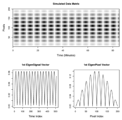
To evaluate the accuracy of our method, we applied it to a simulated data set where we used sine curves to emulate the behavior of typical cell data as shown in Figure 4. Our simulated data matrix, and first EigenSignal and EigenPixel are shown in Figure 10. The data shown in Figure 10 represent the true signal we are trying to recover. Real data, however, have noise and also possess saturated pixels that dampen the signal. To duplicate this behavior, we threshold the data matrix so that everything larger than $0.50$ is replaced by $0.50$; this mimics a saturation at pixel locations that have values larger than $0.50$. To add noise, we introduce realizations from a Gaussian distribution with mean 0 and variance proportional $(u_{i}v_{j})^{2}$. We introduced this variance into the simulated data because it is consistent with the type of variance observed in the real data and we wanted to emulate that behavior. Figure 8 shows the original and saturated first EigenPixel and EigenSignal curves. The first EigenSignal and EigenPixel vectors from the saturated data are both dampened and exaggerated in different regions.

After applying the weighted SVD to the saturated data matrix, we see that upon convergence of the algorithm the resulting first EigenPixel and EigenSignal both come very close to the original curves. The relative error at every pixel and time point are shown on the right panel of Figure 8. When we compare the ratio of the error sum of the saturated over the WSVD Eigen vectors, we see an 11 fold difference in the EigenPixel and a 8 fold difference in the EigenSignal. To see the effect of our weight on the results, we removed the weights and repeated the analysis. Comparing the ratio of the error sum of the saturated over the WSVD Eigen vectors with no weights, only a 1 fold difference in the EigenPixel and a 1 fold difference in the EigenSignal are observed.

6.4 Application of the WSVD to actual data

For illustration we apply the weighted SVD to the pixel-wise matrices of cell 2 from the treated group of low hormone level and cell 11 from the control group of high hormone level. Figure 10 shows the first EigenPixel and EigenSignal of both cell 2 and cell 11. We see that in the peak region of both, between 0–4 minutes into the experiment, there is a large difference in the EigenSignal vectors, especially for cell 11. This is not surprising since most of the saturation occurs in the peak region of the experiment, hence, pixel imputation will mostly affect this region. To further explore this phenomenon, we apply the WSVD only in the peak region (0–4 minutes) and results are also shown in Figure 9. We see that the saturated pixels were dampening the expression in the peak region. This is a key finding since it is believed that $\mathrm{Ca}^{2+}$ expression in this peak region could be used to characterize cells studied.

We have shown that the weighted SVD can be used to clarify the $\mathrm{Ca}^{2+}$ signal in the cells presented. This is an important step when harnessing $\mathrm{Ca}^{2+}$ expression from these cells, especially because $\mathrm{Ca}^{2+}$ expression is dampened drastically if we do not take into account the saturation effect.

7 Comparison of $\mathrm{Ca}^{2+}$ signals: Control and treated

7.1 Initial analysis

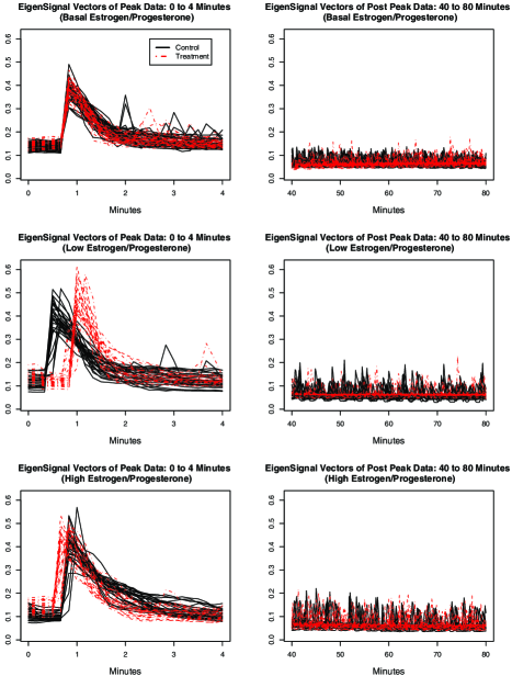
Experience of the third and fourth authors led us to believe that the $\mathrm{Ca}^{2+}$ expression observed immediately after oxytocin exposure is indicative of cell behavior and can predict the response to a given treatment. This leads us to consider use of the “peak” $\mathrm{Ca}^{2+}$ signal and the “post peak” $\mathrm{Ca}^{2+}$ signal, where the “peak” signal is obtained by recovering the signal from the region in the first 4 minutes of the experiment, and the “post peak” $\mathrm{Ca}^{2+}$ signal is harnessed from the region 40–80 minutes after the experiment had begun. One goal is to compare how predictive the initial “peak” $\mathrm{Ca}^{2+}$ signal is compared to the “post peak” $\mathrm{Ca}^{2+}$ signal. In addition, we have the crucial questions (a) how does TCDD affect the cells over all, and (b) how is this response affected by each of the hormone levels in question?

We first take the weighted SVD as described in the previous section and plot the first EigenSignal for every cell and for the “peak” and “post peak” regions; see Figure 11. The first thing to note is that it is easiest to distinguish between the control and treated cell in the low group. The peaks of the first EigenSignals in the low hormone cells do not coincide, so it is quite easy to tell the two groups apart there. About half of the peaks in the high hormone group coincide and all of the peaks of the control and treatment first EigenSignals in the basal hormone group coincide. It is much more difficult to see differences between the control and treated cell lines in the “post peak” region.

Figure 11: First EigenSignal vectors of the “peak” signal (left column ) and the “post peak” signal (right column) obtained from control and treated cells for the three levels of hormone: basal, low and high.

7.2 EigenCells

We next show how to use the SVD a fourth time to extract the effect of the treatment given to the myometrial cells.

One of our goals is to identify differences, if they exist, between control and treated cells. There are many ways in which this comparison can be performed, but we introduce a new way of distinguishing between these two levels of drug. Our approach simply performs an additional SVD on the set of first EigenSignal vectors obtained from the WSVD. Each cell in the experiment is represented by a first EigenSignal vector as shown in Figure 11 and we combine the first EigenSignal vectors of both the treated cells and nontreated cells into three matrices, one per hormone level: basal, low and high. Finally we perform a standard SVD and obtain single value summary points for each cell, or EigenCell values. Each of the three hormone levels correspond to a collection of these one point summaries for a group of cells, which we will call the EigenCell vector. Figure 12 shows the resulting scatter plots of the first two EigenCell vectors. Because almost 100% of the variance is explained by the first two components, we choose to plot only these two. Notice how easy it is to distinguish between the control and treatment groups in the “peak region” for the low and high hormone level. It is much more difficult to separate the control and treatment groups in the “peak” basal hormone level and in all the hormone levels of the “post peak” region.

This clearly shows that the onset of the peak $\mathrm{Ca}^{2+}$ signal in control cells is highly organized and occurs immediately following the oxytocin stimulus in control cells; see Figure 11. In the case of TCDD treated cells that where cultured in low hormone, there is a delayed peak in the $\mathrm{Ca}^{2+}$ signal that is thought to result from suppression of membrane $\mathrm{Ca}^{2+}$ channels and pumps that control the release and/or uptake of intracellular $\mathrm{Ca}^{2+}$. Further, the effects of TCDD on myometrial cells appear to vary as a function of the level of the oxytocin stimulus.

To verify the validity of these claims, we use a 2-fold cross-validation scheme where 80% of the data are used to train the classifier and 20% to test it. For each random split of data into training and test sets, we use a $k$-NN classifier with $k=$ 1–5 nearest neighbors on the training and take the average of the error rates on the test set. The error rates averaged over 1000 runs of the cross validation are shown in Table 1. Notice that the errors reflect our observations, but also show that the “post peak” region could be more useful in the basal hormone level if one tries to predict between the control and treated cell lines.

Table 1: Mean error of 1000 runs of our cross-validation scheme to test the proper classification of the treated and control cell lines using the EigenCell vectors

Hormone level	Peak region	Post peak region
Basal	53%	20%
Low	00%	46%
High	09%	26%

7.3 $\mathrm{Ca}^{2+}$ peak comparison

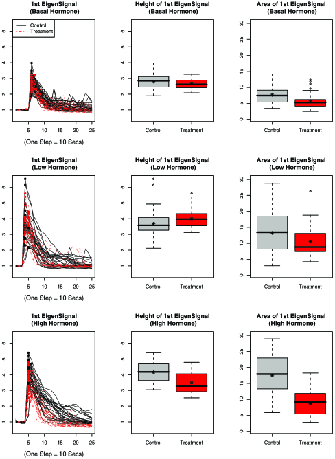
Of course, all these results depend on the original structure of the data, meaning that no manipulation was made to alter the original $\mathrm{Ca}^{2+}$ response other than the imputation of values where saturation occurs. If we wanted to compare the peaks of the initial $\mathrm{Ca}^{2+}$ signal directly, we would have to align the peaks by normalizing them, that is, dividing the EigenSignal by the first 3 initial values, and also perform landmark registration, where the landmark would be the point where the signal begins to rise. Figure 13 shows the normalized and landmarked first EigenSignal curves obtained from the “peak” region after applying the WSVD. A comparison of the peak height and peak area between control and treatment groups is made. By looking at the boxplots in Figure 13, it is reasonable to hypothesize that the mean peak height and area in the control group are greater than those of the treated group. We performed an exact test where we permuted the labels of the peak height and peak area 1,000,000 times. Table 2 shows the resulting test statistic and $p$-value for the peak height and area.

We see a significant difference in the area of the $\mathrm{Ca}^{2+}$ signals when comparing the control and TCDD treated cells. This suggests that TCDD may perturb one or more pathways that regulate $\mathrm{Ca}^{2+}$ entry through channels in the plasma membrane, $\mathrm{Ca}^{2+}$ release from intracellular stores in the endoplasmic reticulum (ER) or other mechanisms to remove $\mathrm{Ca}^{2+}$ from the cytosol by pumps in the plasma membrane or ER membrane. Each of these pathways can now be analyzed in turn to identify the molecular basis for altered $\mathrm{Ca}^{2+}$ signals in these cells and, therefore, the physiological relevance of the decrease in $\mathrm{Ca}^{2+}$ signaling will be determined. Nevertheless, a significant alteration in calcium signaling indicates a significant change in the myometrial cell contractile response.

The differences in peak height, however, seem to be a bit mixed. One important result to note is that for both the peak height and peak area the permutation test is highly significant in the high hormone group, indicating a strong difference between the control and treated cell lines. A decrease in $\mathrm{Ca}^{2+}$ signaling corresponds with a decrease in myometrial contraction (i.e., uterine contraction), and a high level of estrogen/progesterone hormone level in myometrial cells is meant to simulate a response of these cells at the late stages of pregnancy. This means that “normal” function of the uterus could be compromised by TCDD at the late stages of pregnancy, an important finding that deserves further investigation and expansion of our research.

Table 2: Test statistic (difference of mean) between control and treated peak height and peak area and p-values after running permutation tests with 1,000,000 permuted samples

Hormone level	Test stat./$\bolds{p}$-value	Peak height	Peak area
Basal	$\bar{x}_{C}-\bar{x}_{T}$	0.129	1.906
	$p$-value	0.074	0.001
Low	$\bar{x}_{C}-\bar{x}_{T}$	$-0.32$00.	2.710
	$p$-value	0.902	0.046
High	$\bar{x}_{C}-\bar{x}_{T}$	0.669	8.883
	$p$-value	0.000	0.000

Figure 12: A scatter plot of the first and second EigenCell vectors for the “peak” region (left column) and the“post peak” region (right column). The control ‘$\circ$’ and treated ‘$+$’ groups are shown for the three levels of hormone: basal, low and high.

Figure 13: Left column: Normalized and landmarked first EigenSignal vectors of the “peak” region in the control and treated cells for each of the three hormone levels: basal, low and high. Middle column: Boxplots of the peak height for the control and treated cells in each of the three hormone levels: basal, low and high. Right column: Boxplots of the area in the “peak” region for the control and treated cells in each of the three hormone levels: basal, low and high.

8 Conclusion

In this work we use the SVD in four different ways:

1. []

2. First, we use it to detect the $\mathrm{Ca}^{2+}$ signal by using the initial first EigenPixel vector. This approach summarizes cell location information across all 512 images instead of using only one image as is typically done for these data.

3. Second, another SVD was then used to extract the $\mathrm{Ca}^{2+}$ signal from the pixel-wise matrix derived after segmenting the cell region in raw images. These first EigenSignal and first EigenPixel vectors serve as the templates used to “clean up” the signal.

4. Third, we used those candidate EigenSignal and EigenPixel vectors to clarify the $\mathrm{Ca}^{2+}$ signal by applying a new weighted SVD, the WSVD, to impute values where saturation occurs in the signal.

5. Finally, we use the singular value decomposition once more to discriminate between control and treated EigenSignal vectors resulting from the WSVD. We summarize the variation in the control and treated cell lines by capturing the variability of each cell into one value per cell, giving us the EigenCell vector.

To our knowledge $\mathrm{Ca}^{2+}$ signal detection, extraction, clarification and comparison using the SVD has not been previously performed. These four applications of the singular value decomposition to analyze $\mathrm{Ca}^{2+}$ signaling in myometrial cells show its utility and flexibility for analyzing complex $\mathrm{Ca}^{2+}$ signals such as oscillations and waves.

An additional finding is that saturation undermines the $\mathrm{Ca}^{2+}$ signal obtained by simply averaging the pixels representing the cell. Correcting the effects of saturation must be an integral step while studying these type of data. Moreover, the hypothesized importance of the “peak” region as being a way of characterizing cells of this type seems to be a valid claim. From our analysis we were able to clearly distinguish between the treated and control groups by using the area in the “peak” region and by using the scatter plots of EigenCells vectors obtained in our fourth and final application of the SVD.

To conclude, we have shown the importance of the initial peak in $\mathrm{Ca}^{2+}$ signaling of myometrial cells by the SVD, and also exhibit new uses of the SVD to segment, extract, clarify and compare $\mathrm{Ca}^{2+}$ signals in this context.

[id=suppA] Supplement A Calcium ion signaling movies with TCDD exposure [doi]10.1214/07-AOAS253SUPPA .zip [url]http://lib.stat.cmu.edu/aoas/253/dir2_T.zip When unzipped, the movie is in .avi format, and is 30 MB in size. One can view it, for example, using windows media player.

[id=suppB] Supplement B Calcium ion signaling movies without TCDD exposure [doi]10.1214/07-AOAS253SUPPB .zip [url]http://lib.stat.cmu.edu/aoas/253/dir2_C.zip When unzipped, the movie is in .avi format, and is 40 MB in size. One can view it, for example, using windows media player.

References

- (1) Alter, O., Brown, P. O. and Botstein, D. (2000). Singular value decomposition for genome-wide expression data processing and modeling. Proc. Natl. Acad. Sci. 97 10101–10106.
- (2) Barhoumi, R., Awooda, I., Mouneimne, Y., Safe, S. and Burghardt, R. C. (2006). Effects of benzo-a-pyrene on oxytocin-induced oscillations in myometrial cells. Toxicol. Lett. 165 133–141.
- (3) Barhoumi, R., Mouneimne, Y., Awooda, I., Safe, S., Donnelly, K. C. and Burghardt, R. C. (2002). Characterization of calcium oscillations in normal and Benzo[a]pyrene-treated clone 9 cells. Toxicol. Sci. 68 444–450.
- (4) Beckers, J. and Rixen, M. (2003). Eof calculations and data filling from incomplete oceanographic datasets. J. Atmos. Oceanic Technol. 20 1839–1856.
- (5) Burghardt, R. C., Barhoumi, R., Sanborn, B. M. and Andersen, J. (1999). Oxytocin-induced responses in human myometrial cells. Biol. Reprod. 60 777–782.
- (6) Gabriel, K. R. and Zamir, S. (1979). Lower rank approximation of matrices by least squares with any choice of weights. Technometrics 21 489–498.
- (7) Kurucz, M., Benczúr, A. A. and Csalogány, K. (2007). Methods for large scale SVD with missing values. Proceedings of the KDD Cup and Workshop 2007. Available at: http://www.cs.uic.edu/~liub/KDD-cup-2007/proceedings.html.
- (8) Liu, L., Hawkins, D. M., Ghosh, S. and Young, S. S. (2003). Robust singular value decomposition analysis of microarray data. PNAS 100 13167–13172. \MR2016727
- (9) Putney, J. W. (1998). Calcium signaling: Up, down, up, down what’s the point? Science 279 191–192.
- (10) R Development Core Team (2008). R: A Language and Environment for Statistical Computing. R Foundation for Statistical Computing, Vienna, Austria. Available at http://www.r-project.org.
- (11) Ruhe, A. (1974). Numerical computation of principal components when several observations are missing. Technical report, UMINF-48, Umeå, Sweden.
- (12) Sneyd, J., Keizer, J. and Sanderson, M. J. (1995). Mechanisms of calcium oscillations and waves: A quantitative analysis. FASEB J. 9 1463–1472.
- (13) Trefethen, L. N. and Bau III, D. (1997). Numerical Linear Algebra. SIAM, Philadelphia. \MR1444820
- (14) Troyanskaya, O. G., Cantor, M., Sherlock, G., Brown, P. O., Hastie, T., Tibshirani R., Botstein, D. and Altman, R. B. (2001). Missing value estimation methods for dna microarrays. Bioinformatics 17 520–525.