Square-root lasso: pivotal recovery of sparse signals via conic programming
Abstract.
We propose a pivotal method for estimating high-dimensional sparse linear regression models, where the overall number of regressors is large, possibly much larger than , but only regressors are significant. The method is a modification of the lasso, called the square-root lasso. The method is pivotal in that it neither relies on the knowledge of the standard deviation or nor does it need to pre-estimate . Moreover, the method does not rely on normality or sub-Gaussianity of noise. It achieves near-oracle performance, attaining the convergence rate in the prediction norm, and thus matching the performance of the lasso with known . These performance results are valid for both Gaussian and non-Gaussian errors, under some mild moment restrictions. We formulate the square-root lasso as a solution to a convex conic programming problem, which allows us to implement the estimator using efficient algorithmic methods, such as interior-point and first-order methods.
1. Introduction
We consider the linear regression model for outcome given fixed -dimensional regressors :
| (1) |
with independent and identically distributed noise having law such that
| (2) |
The vector is the unknown true parameter value, and is the unknown standard deviation. The regressors are -dimensional, where the dimension is possibly much larger than the sample size . Accordingly, the true parameter value lies in a very high-dimensional space . However, the key assumption that makes the estimation possible is the sparsity of :
| (3) |
The identity of the significant regressors is unknown. Throughout, without loss of generality, we normalize
| (4) |
In making asymptotic statements below we allow for and as .
The ordinary least squares estimator is not consistent for estimating in the setting with . The lasso estimator [23] can restore consistency under mild conditions by penalizing through the sum of absolute parameter values:
| (5) |
where and . The lasso estimator is computationally attractive because it minimizes a structured convex function. Moreover, when errors are normal, , and suitable design conditions hold, if one uses the penalty level
| (6) |
for some constant , this estimator achieves the near-oracle performance, namely
| (7) |
with probability at least . Remarkably, in (7) the overall number of regressors shows up only through a logarithmic factor, so that if is polynomial in , the oracle rate is achieved up to a factor of . Recall that the oracle knows the identity of significant regressors, and so it can achieve the rate . Result (7) was demonstrated by [4], and closely related results were given in [13], and [28]. [6], [25], [10], [5], [30], [8], [27], and [29] contain other fundamental results obtained for related problems; see [4] for further references.
Despite these attractive features, the lasso construction (5) – (6) relies on knowing the standard deviation of the noise. Estimation of is non-trivial when is large, particularly when , and remains an outstanding practical and theoretical problem. The estimator we propose in this paper, the square-root lasso, eliminates the need to know or to pre-estimate . In addition, by using moderate deviation theory, we can dispense with the normality assumption under certain conditions.
The square-root lasso estimator of is defined as the solution to the optimization problem
| (8) |
with the penalty level
| (9) |
for some constant . The penalty level in (9) is independent of , in contrast to (6), and hence is pivotal with respect to this parameter. Furthermore, under reasonable conditions, the proposed penalty level (9) will also be valid asymptotically without imposing normality , by virtue of moderate deviation theory.
We will show that the square-root lasso estimator achieves the near-oracle rates of convergence under suitable design conditions and suitable conditions on that extend significantly beyond normality:
| (10) |
with probability approaching . Thus, this estimator matches the near-oracle performance of lasso, even though the noise level is unknown. This is the main result of this paper. It is important to emphasize here that this result is not a direct consequence of the analogous result for the lasso. Indeed, for a given value of the penalty level, the statistical structure of the square-root lasso is different from that of the lasso, and so our proofs are also different.
Importantly, despite taking the square-root of the least squares criterion function, the problem (8) retains global convexity, making the estimator computationally attractive. The second main result of this paper is to formulate the square-root lasso as a solution to a conic programming problem. Conic programming can be seen as linear programming with conic constraints, so it generalizes canonical linear programming with non-negative orthant constraints, and inherits a rich set of theoretical properties and algorithmic methods from linear programming. In our case, the constraints take the form of a second-order cone, leading to a particular, highly tractable, form of conic programming. In turn, this allows us to implement the estimator using efficient algorithmic methods, such as interior-point methods, which provide polynomial-time bounds on computational time [16, 17], and modern first-order methods [14, 15, 11, 1].
In what follows, all true parameter values, such as , , , are implicitly indexed by the sample size , but we omit the index in our notation whenever this does not cause confusion. The regressors are taken to be fixed throughout. This includes random design as a special case, where we condition on the realized values of the regressors. In making asymptotic statements, we assume that and , and we also allow for . The notation is defined with respect to . We use the notation , and . The -norm is denoted by , and norm by . Given a vector and a set of indices , we denote by the vector in which if , if . We also use . We use to denote for some constant that does not depend on .
2. The choice of penalty level
2.1. The general principle and heuristics
The key quantity determining the choice of the penalty level for square-root lasso is the score, the gradient of evaluated at the true parameter value :
The score does not depend on the unknown standard deviation or the unknown true parameter value , and therefore is pivotal with respect to . Under the classical normality assumption, namely , the score is in fact completely pivotal, conditional on . This means that in principle we know the distribution of in this case, or at least we can compute it by simulation.
The score summarizes the estimation noise in our problem, and we may set the penalty level to overcome it. For reasons of efficiency, we set at the smallest level that dominates the estimation noise, namely we choose the smallest such that
| (11) |
with a high probability, say , where is the maximal score scaled by , and is a theoretical constant of [4] to be stated later. The principle of setting to dominate the score of the criterion function is motivated by [4]’s choice of penalty level for the lasso. This general principle carries over to other convex problems, including ours, and that leads to the optimal, near-oracle, performance of other -penalized estimators.
In the case of the square-root lasso the maximal score is pivotal, so the penalty level in (11) must also be pivotal. We used the square-root transformation in the square-root lasso formulation (8) precisely to guarantee this pivotality. In contrast, for lasso, the score is obviously non-pivotal, since it depends on . Thus, the penalty level for lasso must be non-pivotal. These theoretical differences translate into obvious practical differences. In the lasso, we need to guess conservative upper bounds on , or we need to use preliminary estimation of using a pilot lasso, which uses a conservative upper bound on . In the square-root lasso, none of these is needed. Finally, the use of pivotality principle for constructing the penalty level is also fruitful in other problems with pivotal scores, for example, median regression [3].
The rule (11) is not practical, since we do not observe directly. However, we can proceed as follows:
1. When we know the distribution of errors exactly, e.g., , we propose to set as times the quantile of given . This choice of the penalty level precisely implements (11), and is easy to compute by simulation.
2. When we do not know exactly, but instead know that is an element of some family , we can rely on either finite-sample or asymptotic upper bounds on quantiles of given . For example, as mentioned in the introduction, under some mild conditions on , is a valid asymptotic choice.
What follows below elaborates these approaches. Before describing the details, it is useful to mention some heuristics for the principle (11). These arise from considering the simplest case, where none of the regressors are significant, so that . We want our estimator to perform at a near-oracle level in all cases, including this one. Here the oracle estimator is . We also want in this case, at least with a high probability . From the subgradient optimality conditions of (8), in order for this to be true we must have . We can only guarantee this by setting the penalty level such that with probability at least . This is precisely the rule (11), and, as it turns out, this delivers near-oracle performance more generally, when .
2.2. The formal choice of penalty level and its properties
In order to describe our choice of formally, define for
| (12) | |||
| (13) |
where , with independent and identically distributed having law . We can compute (12) by simulation.
In the normal case, , can be either of
| (14) |
which we call here the exact and asymptotic options, respectively. The parameter is a confidence level which guarantees near-oracle performance with probability ; we recommend . The constant is a theoretical constant of [4], which is needed to guarantee a regularization event introduced in the next section; we recommend . The options in (14) are valid either in finite or large samples under the conditions stated below. They are also supported by the finite-sample experiments reported in Section C. We recommend using the exact option over the asymptotic option, because by construction the former is better tailored to the given sample size and design matrix . Nonetheless, the asymptotic option is easier to compute. Our theoretical results in section 3 show that the options in (14) lead to near-oracle rates of convergence.
For the asymptotic results, we shall impose the following condition:
Condition G. We have that and as .
The following lemma shows that the exact and asymptotic options in (14) implement the regularization event in the Gaussian case with the exact or asymptotic probability respectively. The lemma also bounds the magnitude of the penalty level for the exact option, which will be useful for stating bounds on the estimation error. We assume throughout the paper that is bounded away from 1, but we allow to approach as grows.
Lemma 1.
In the non-normal case, can be any of
| (15) |
which we call the exact, semi-exact, and asymptotic options, respectively. We set the confidence level and the constant as before. The exact option is applicable when , as for example in the previous normal case. The semi-exact option is applicable when is a member of some family , or whenever the family gives a more conservative penalty level. We also assume that in (36) is either finite or, more generally, that the maximum in (36) is well defined. For example, in applications, where the regression errors are thought of having a potentially wide range of tail behavior, it is useful to set where denotes the Student distribution with degrees of freedom. As stated previously, we can compute the quantiles by simulation. Therefore, we can implement the exact option easily, and if is not too large, we can also implement the semi-exact option easily. Finally, the asymptotic option is applicable when and design satisfy Condition M and has the advantage of being trivial to compute.
For the asymptotic results in the non-normal case, we impose the following moment conditions.
Condition M. There exist a finite constant such that the law is an element of the family
such that the design obeys
We also have to restrict the growth of relative to , and we also assume that is either bounded away from zero or approaches zero not too rapidly. See also the Supplementary Material for an alternative condition.
Condition R. As , for some constant , and , where is defined in Condition M.
The following lemma shows that the options (36) implement the regularization event in the non-Gaussian case with exact or asymptotic probability . In particular, Conditions R and M, through relations (32) and (34), imply that for any fixed ,
| (16) |
The lemma also bounds the magnitude of the penalty level for the exact and semi-exact options, which is useful for stating bounds on the estimation error in section 3.
Lemma 2.
(i) The exact option in (36) implements with probability at least , if . (ii) The semi-exact option in (36) implements with probability at least , if either or for some . Suppose further that Conditions M and R hold. Then, (iii) the asymptotic option in (36) implements with probability at least , and (iv) the magnitude of the penalty level of the exact and semi-exact options in (36) satisfies the inequality
Thus all of the asymptotic conclusions reached in Lemma 1 about the penalty level in the Gaussian case continue to hold in the non-Gaussian case, albeit under more restricted conditions on the growth of relative to . The growth condition depends on the number of bounded moments of regressors and the error terms: the higher is, the more rapidly can grow with . We emphasize that Conditions M and R are only one possible set of sufficient conditions that guarantees the Gaussian-like conclusions of Lemma 2. We derived them using the moderate deviation theory of [22]. For example, in the Supplementary Material, we provide an alternative condition, based on the use of the self-normalized moderate deviation theory of [9], which results in much weaker growth condition on in relation to , but requires much stronger conditions on the moments of regressors.
3. Finite-sample and asymptotic bounds on the estimation error
3.1. Conditions on the Gram matrix
We shall state convergence rates for in the Euclidean norm and also in the prediction norm
The latter norm directly depends on the Gram matrix . The choice of penalty level described in Section 2 ensures the regularization event , with probability or with probability approaching . This event will in turn imply another regularization event, namely that belongs to the restricted set , where
Accordingly, we will state the bounds on estimation errors and in terms of the following restricted eigenvalues of the Gram matrix :
| (17) |
These restricted eigenvalues can depend on and , but we suppress the dependence in our notation.
In making simplified asymptotic statements, such as those appearing in Section 1, we invoke the following condition on the restricted eigenvalues:
Condition RE. There exist finite constants and , such that the restricted eigenvalues obey for all .
The restricted eigenvalues (17) are simply variants of the restricted eigenvalues introduced in [4]. Even though the minimal eigenvalue of the Gram matrix is zero whenever , [4] show that its restricted eigenvalues can be bounded away from zero, and they and others provide sufficient primitive conditions that cover many fixed and random designs of interest, which allow for reasonably general, though not arbitrary, forms of correlation between regressors. This makes conditions on restricted eigenvalues useful for many applications. Consequently, we take the restricted eigenvalues as primitive quantities and Condition RE as primitive. The restricted eigenvalues are tightly tailored to the -penalized estimation problem. Indeed, is the modulus of continuity between the estimation norm and the penalty-related term computed over the restricted set, containing the deviation of the estimator from the true value; and is the modulus of continuity between the estimation norm and the Euclidean norm over this set.
It is useful to recall at least one simple sufficient condition for bounded restricted eigenvalues. If for , the –sparse eigenvalues of the Gram matrix are bounded away from zero and from above for all , i.e.,
| (18) |
for some positive finite constants , , and , then Condition RE holds once is sufficiently large. In words, (18) only requires the eigenvalues of certain small submatrices of the large Gram matrix to be bounded from above and below. The sufficiency of (18) for Condition RE follows from [4], and many sufficient conditions for (18) are provided by [4], [28], [13], and [20].
3.2. Finite-sample and asymptotic bounds on estimation error
We now present the main result of this paper. Recall that we do not assume that the noise is sub-Gaussian or that is known.
Theorem 1.
This result provides a finite-sample bound for that is similar to that for the lasso estimator with known , and this result leads to the same rates of convergence as in the case of lasso. It is important to note some differences. First, for a given value of the penalty level , the statistical structure of square-root lasso is different from that of lasso, and so our proof of Theorem 1 is also different. Second, in the proof we have to invoke the additional growth restriction, , which is not present in the lasso analysis that treats as known. We may think of this restriction as the price of not knowing in our framework. However, this additional condition is very mild and holds asymptotically under typical conditions if , as the corollaries below indicate, and it is independent of . In comparison, for the lasso estimator, if we treat as unknown and attempt to estimate it consistently using a pilot lasso, which uses an upper bound instead of , a similar growth condition would have to be imposed, but this condition depends on and is more restrictive than our growth condition when is large.
Theorem 1 implies the following bounds when combined with Lemma 1, Lemma 2, and the concentration property (16).
Corollary 1.
Corollary 2.
Corollary 3.
As in Lemma 2, in order to achieve Gaussian-like asymptotic conclusions in the non-Gaussian case, we impose stronger restrictions on the growth of relative to .
4. Computational properties of square-root lasso
The second main result of this paper is to formulate the square-root lasso as a conic programming problem, with constraints given by a second-order cone, also informally known as the ice-cream cone. This allows us to implement the estimator using efficient algorithmic methods, such as interior-point methods, which provide polynomial-time bounds on computational time [16, 17], and modern first-order methods that have been recently extended to handle very large conic programming problems [14, 15, 11, 1]. Before describing the details, it is useful to recall that a conic programming problem takes the form subject to and , where is a cone. Conic programming has a tractable dual form subject to and , where is the dual cone of . A particularly important, highly tractable class of problems arises when is the ice-cream cone, , which is self-dual, .
The square-root lasso optimization problem is precisely a conic programming problem with second-order conic constraints. Indeed, we can reformulate (8) as follows:
| (19) |
Furthermore, we can show that this problem admits the following strongly dual problem:
| (20) |
Recall that strong duality holds between a primal and its dual problem if their optimal values are the same, i.e., there is no duality gap. This is typically an assumption needed for interior-point methods and first-order methods to work. From a statistical perspective, this dual problem maximizes the sample correlation of the score variable with the outcome variables subject to the constraint that the score is approximately uncorrelated with the covariates . The optimal scores equal the residuals , for all , up to a renormalization factor; they play a key role in deriving sparsity bounds on . We formalize the preceding discussion in the following theorem.
Theorem 2.
The conic formulation and the strong duality demonstrated in Theorem 2 allow us to employ both the interior-point and first-order methods for conic programs to compute the square-root lasso. We have implemented both of these methods, as well as a coordinatewise method, for the square-root lasso and made the code available through the authors’ webpages. The square-root lasso runs at least as fast as the corresponding implementations of these methods for the lasso, for instance, the Sdpt3 implementation of interior-point method [24], and the Tfocs implementation of first-order methods by Becker, Candès and Grant described in [2]. We report the exact running times in the Supplementary Material.
5. Empirical performance of square-root lasso relative to lasso
In this section we use Monte Carlo experiments to assess the finite sample performance of (i) the infeasible lasso with known which is unknown outside the experiments, (ii) the post infeasible lasso, which applies ordinary least squares to the model selected by infeasible lasso, (iii) the square-root lasso with unknown , and (iv) the post square-root lasso, which applies ordinary least squares to the model selected by square-root lasso.
We set the penalty level for the infeasible lasso and the square-root lasso according to the asymptotic options (6) and (9) respectively, with and . We have also performed experiments where we set the penalty levels according to the exact option. The results are similar, so we do not report them separately.
We use the linear regression model stated in the introduction as a data-generating process, with either standard normal or errors: (a) , , so that in either case. We set the true parameter value as and vary between and . The number of regressors is , the sample size is , and we used simulations for each design. We generate regressors as with the Toeplitz correlation matrix . We use as benchmark the performance of the oracle estimator with known true support of which is unknown outside the experiment.
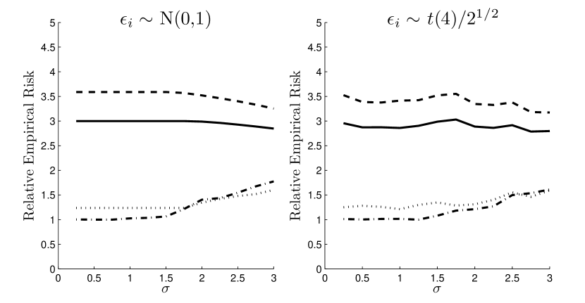
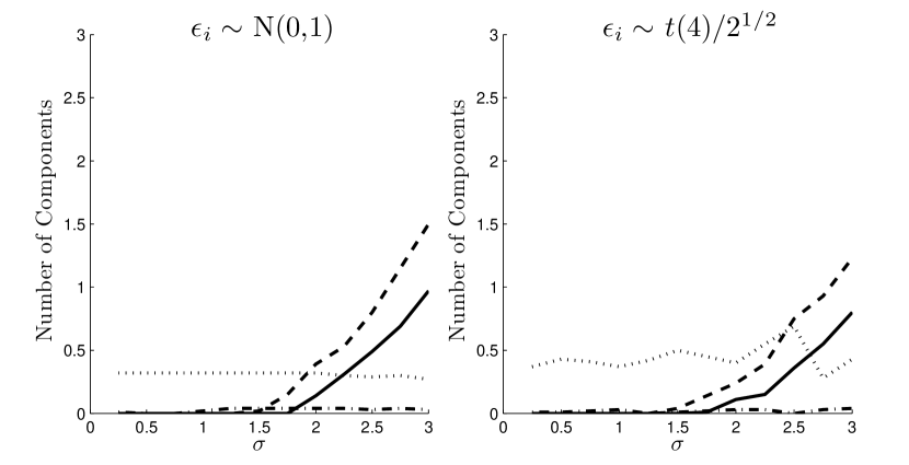
We present the results of computational experiments for designs (a) and (b) in Figs. 5 and 2. For each model, Figure 5 shows the relative average empirical risk with respect to the oracle estimator , , and Figure 2 shows the average number of regressors missed from the true model and the average number of regressors selected outside the true model, and , respectively.
Figure 5 shows the empirical risk of the estimators. We see that, for a wide range of the noise level , the square-root lasso with unknown performs comparably to the infeasible lasso with known . These results agree with our theoretical results, which state that the upper bounds on empirical risk for the square-root lasso asymptotically approach the analogous bounds for infeasible lasso. The finite-sample differences in empirical risk for the infeasible lasso and the square-root lasso arise primarily due to the square-root lasso having a larger bias than the infeasible lasso. This bias arises because the square-root lasso uses an effectively heavier penalty induced by in place of ; indeed, in these experiments, the average values of varied between and .
Figure 5 shows that the post square-root lasso substantially outperforms both the infeasible lasso and the square-root lasso. Moreover, for a wide range of , the post square-root lasso outperforms the post infeasible lasso. The post square-root lasso is able to improve over the square-root lasso due to removal of the relatively large shrinkage bias of the square-root lasso. Moreover, the post square-root lasso is able to outperform the post infeasible lasso primarily due to its better sparsity properties, which can be observed from Figure 2. These results on the post square-root lasso agree closely with our theoretical results reported in the arXiv working paper “Pivotal Estimation of Nonparametric Functions via Square-root Lasso” by the authors, which state that the upper bounds on empirical risk for the post square-root lasso asymptotically are no larger than the analogous bounds for the square-root lasso or the infeasible lasso, and can be strictly better when the square-root lasso acts as a near-perfect model selection device. We see this happening in Figure 5, where as the noise level decreases, the post square-root lasso starts to perform as well as the oracle estimator. As we see from Figure 2, this happens because as decreases, the square-root lasso starts to select the true model nearly perfectly, and hence the post square-root lasso starts to become the oracle estimator with a high probability.
Next let us now comment on the difference between the normal and noise cases, i.e., between the right and left panels in Figure 5 and 2. We see that the results for the Gaussian case carry over to case with nearly undetectable changes. In fact, the performance of the infeasible lasso and the square-root lasso under errors nearly coincides with their performance under Gaussian errors, as predicted by our theoretical results in the main text, using moderate deviation theory, and in the Supplementary Material, using self-normalized moderate deviation theory.
In the Supplementary Material, we provide further Monte Carlo comparisons that include asymmetric error distributions, highly correlated designs, and feasible lasso estimators based on the use of conservative bounds on and cross validation. Let us briefly summarize the key conclusions from these experiments. First, presence of asymmetry in the noise distribution and of a high correlation in the design does not change the results qualitatively. Second, naive use of conservative bounds on does not result in good feasible lasso estimators. Third, the use of cross validation for choosing the penalty level does produce a feasible lasso estimator performing well in terms of empirical risk but poorly in terms of model selection. Nevertheless, even in terms of empirical risk, the cross-validated lasso is outperformed by the post square-root lasso. In addition, cross-validated lasso is outperformed by the square-root-lasso with the penalty level scaled by 1/2. This is noteworthy, since the estimators based on the square-root lasso are much cheaper computationally. Lastly, in the 2011 arXiv working paper “Pivotal Estimation of Nonparametric Functions via Square-Root Lasso” we provide a further analysis of the post square-root lasso estimator and generalize the setting of the present paper to the fully nonparametric regression model.
Acknowledgement
We would like to thank Isaiah Andrews, Denis Chetverikov, Joseph Doyle, Ilze Kalnina, and James MacKinnon for very helpful comments. The authors also thank the editor and two referees for suggestions that greatly improved the paper. This work was supported by the National Science Foundation.
Supplementary Material
The online Supplementary Material contains a complementary analysis of the penalty choice based on moderate deviation theory for self-normalizing sums, discussion on computational aspects of square-root lasso as compared to lasso, and additional Monte Carlo experiments. We also provide the omitted part of proof of Lemma 2, and list the inequalities used in the proofs.
Appendix 1
Proofs of Theorems 1 and 2
Proof of Theorem 1.
Step 1. We show that under the prescribed penalty level. By definition of
| (21) |
where the last inequality holds because
| (22) |
Also, if then
| (23) |
where the first inequality hold by convexity of . Combining (21) with (23) we obtain
| (24) |
that is
| (25) |
Proof of Theorem 2.
The equivalence of square-root lasso problem (8) and the conic programming problem (19) follows immediately from the definitions. To establish the duality, for , we can write (19) in matrix form as
By the conic duality theorem, this has dual
The constraints and leads to . The conic constraint leads to . By scaling the variable by we obtain the stated dual problem.
Since the primal problem is strongly feasible, strong duality holds by Theorem 3.2.6 of [17]. Thus, by strong duality, we have Since for every , we have
Rearranging the terms we have . If , since , the equality can only hold for . ∎
Appendix 2
Proofs of Lemmas 1 and 2
Proof of Lemma 1.
Statement (i) holds by definition. To show statement (ii), we define and . It is known that when . Then since for each , conditional on , we have by the union bound and , Statement (ii) follows by observing that by Chernoff tail bound for , Lemma 1 in [12], , and
where we have used the inequality for .
For statement (iii), it is sufficient to show that . It can be seen that there exists a such that and so that Proceeding as before, by Chernoff tail bound for , and
Putting the inequalities together, we conclude that .
Finally, the asymptotic result follows directly from the finite sample bounds and noting that and that under the growth condition we can choose so that . ∎
Proof of Lemma 2.
Statements (i) and (ii) hold by definition. To show (iii), consider first the case of , and define and for some which grows to infinity but so slowly that the condition stated below is satisfied. Then for any and that obey Condition M:
where (1) holds by the union bound; (2) holds by the application of either Rosenthal’s inequality (Rosenthal 1970) for the case of and Vonbahr–Esseen’s inequalities (von Bahr & Esseen 1965) for the case of ,
| (32) |
(4) and (6) by as ; (5) by , which holds if Under our condition , this condition is satisfied for some slowly growing , if
| (33) |
To verify relation (3), by Condition M and Slastnikov’s theorem on moderate deviations, see [22] and [19], we have that uniformly in for some , uniformly in and for any , so the relation (3) holds for for by Condition R. We apply Slastnikov’s theorem to for , where we allow the design , the law , and index to be indexed by . Slastnikov’s theorem then applies provided which is implied by our Condition M, and where we used the condition that the design is fixed, so that are independent of . Thus, we obtained the moderate deviation result uniformly in and for any sequence of distributions and designs that obey our Condition M.
Next suppose that . Then the same argument applies, except that now relation (2) could also be established by using Slastnikov’s theorem on moderate deviations. In this case redefine then, for some constant we have
| (34) |
so the relation (2) holds if
| (35) |
This applies whenever , and this results in weaker requirements on if . The relation (5) then follows if , which is easily satisfied for the new , and the result follows.
Combining conditions in (33) and (35) to give the weakest restrictions on the growth of , we obtain the growth conditions stated in the lemma.
To show statement (iv) of the lemma, it suffices to show that for any , and , , which follows analogously to the proof of statement (iii); we relegate the details to the Supplementary Material. ∎
References
- [1] A. Beck and M. Teboulle. A fast iterative shrinkage-thresholding algorithm for linear inverse problems. SIAM J. Imaging Sciences, 2(1):183–202, 2009.
- [2] Stephen Becker, Emmanuel Candès, and Michael Grant. Templates for convex cone problems with applications to sparse signal recovery. ArXiv, 2010.
- [3] A. Belloni and V. Chernozhukov. -penalized quantile regression for high dimensional sparse models. Ann. Statist., 39(1):82–130, 2011.
- [4] P. J. Bickel, Y. Ritov, and A. B. Tsybakov. Simultaneous analysis of Lasso and Dantzig selector. Ann. Statist., 37(4):1705–1732, 2009.
- [5] F. Bunea, A. B. Tsybakov, and M. H. Wegkamp. Aggregation for Gaussian regression. Ann. Statist., 35(4):1674–1697, 2007.
- [6] E. Candès and T. Tao. The Dantzig selector: statistical estimation when is much larger than . Ann. Statist., 35(6):2313–2351, 2007.
- [7] V. H. de la Peña, T. L. Lai, and Q.-M. Shao. Self-Normalized Processes. Springer, 2009.
- [8] J. Huang, J. L. Horowitz, and S. Ma. Asymptotic properties of bridge estimators in sparse high-dimensional regression models. Ann. Statist., 36(2):587 613, 2008.
- [9] B. Y. Jing, Q. M. Shao, and Q. Y. Wang. Self-normalized Cramér type large deviations for independent random variables. Ann. Probab., 31:2167–2215, 2003.
- [10] V. Koltchinskii. Sparsity in penalized empirical risk minimization. Ann. Inst. H. Poincar Probab. Statist., 45(1):7–57, 2009.
- [11] G. Lan, Z. Lu, and R. D. C. Monteiro. Primal-dual first-order methods with interation-complexity for cone programming. Mathematical Programming, (126):1–29, 2011.
- [12] B. Laurent and P. Massart. Adaptive estimation of a quadratic functional by model selection. Ann. Statist., 28(5):1302–1338, 2000.
- [13] N. Meinshausen and B. Yu. Lasso-type recovery of sparse representations for high-dimensional data. Ann. Statist., 37(1):2246–2270, 2009.
- [14] Y. Nesterov. Smooth minimization of non-smooth functions, mathematical programming. Mathematical Programming, 103(1):127–152, 2005.
- [15] Y. Nesterov. Dual extrapolation and its applications to solving variational inequalities and related problems. Mathematical Programming, 109(2-3):319–344, 2007.
- [16] Y. Nesterov and A Nemirovskii. Interior-Point Polynomial Algorithms in Convex Programming. Society for Industrial and Applied Mathematics (SIAM), Philadelphia, 1993.
- [17] J. Renegar. A Mathematical View of Interior-Point Methods in Convex Optimization. Society for Industrial and Applied Mathematics (SIAM), Philadelphia, 2001.
- [18] H. P. Rosenthal. On the subspaces of spanned by sequences of independent random variables. Israel J. Math., 9:273 –303, 1970.
- [19] Herman Rubin and J. Sethuraman. Probabilities of moderatie deviations. Sankhyā Ser. A, 27:325–346, 1965.
- [20] Mark Rudelson and Roman Vershynin. On sparse reconstruction from Fourier and Gaussian measurements. Comm. Pure and Applied Mathematics, 61:1025 –1045, 2008.
- [21] A. D. Slastnikov. Limit theorems for moderate deviation probabilities. Theory of Probability and its Applications, 23:322–340, 1979.
- [22] A. D. Slastnikov. Large deviations for sums of nonidentically distributed random variables. Teor. Veroyatnost. i Primenen., 27(1):36–46, 1982.
- [23] R. Tibshirani. Regression shrinkage and selection via the lasso. J. Roy. Statist. Soc. Ser. B, 58:267–288, 1996.
- [24] K. C. Toh, M. J. Todd, and R. H. Tutuncu. On the implementation and usage of sdpt3 – a matlab software package for semidefinite-quadratic-linear programming, version 4.0. Handbook of Semidefinite, Cone and Polynomial Optimization: Theory, Algorithms, Software and Applications, Edited by M. Anjos and J.B. Lasserre, June 2010.
- [25] S. A. van de Geer. High-dimensional generalized linear models and the lasso. Ann. Statist., 36(2):614–645, 2008.
- [26] Bengt von Bahr and Carl-Gustav Esseen. Inequalities for the rth absolute moment of a sum of random variables, . Ann. Math. Statist, 36:299–303, 1965.
- [27] M. Wainwright. Sharp thresholds for noisy and high-dimensional recovery of sparsity using -constrained quadratic programming (lasso). IEEE Transactions on Information Theory, 55:2183–2202, May 2009.
- [28] C.-H. Zhang and J. Huang. The sparsity and bias of the lasso selection in high-dimensional linear regression. Ann. Statist., 36(4):1567–1594, 2008.
- [29] Tong Zhang. On the consistency of feature selection using greedy least squares regression. J. Machine Learning Research, 10:555–568, 2009.
- [30] P. Zhao and B. Yu. On model selection consistency of lasso. J. Machine Learning Research, 7:2541–2567, Nov. 2006.
Supplementary Appendix for “Square-root lasso: pivotal recovery of sparse signals via conic programming”
Abstract. In this appendix we gather additional theoretical and computational results for “Square-root lasso: pivotal recovery of sparse signals via conic programming.” We include a complementary analysis of the penalty choice based on moderate deviation theory for self-normalizing sums. We provide a discussion on computational aspects of square-root lasso as compared to lasso. We carry out additional Monte Carlo experiments. We also provide the omitted part of proof of Lemma 2, and list the inequalities used in the proofs.
Appendix A Additional Theoretical Results
In this section we derive additional results using moderate deviation theory for self-normalizing sums to bound the penalty level. These results are complementary to the results given in the main text since conditions required here are not implied nor imply the conditions there. These conditions require stronger moment assumptions but in exchange they result in weaker growth requirements on in relation to .
Recall the definition of the choices of penalty levels
| (36) |
where -quantile of . We will make use of the following condition.
Condition SN. There is a such that the noise obeys and the design obeys . Moreover, we also assume and ().
Lemma 3.
Suppose that condition SN holds and . Then, (1) the asymptotic option in (36) implements with probability at least , and (2)
This lemma in combination with Theorem 1 of the main text imply the following result:
Corollary 4.
Consider the model described in the main text. Suppose that Conditions RE and SN hold, and as . Let be specified according to the asymptotic or exact option in (36). There is an term such that with probability at least
Appendix B Additional Computational Results
B.1. Overview of Additional Computational Results
In the main text we formulated the square-root lasso as a convex conic programming problem. This fact allows us to use conic programming methods to compute the square-root lasso estimator. In this section we provide further details on these methods, specifically on (i) the first-order methods, (ii) the interior-point methods, and (iii) the componentwise search methods, as specifically adapted to solving conic programming problems. We shall also compare the adaptation of these methods to square-root lasso with the respective adaptation of these methods to lasso.
B.2. Computational Times
Our main message here is that the average running times for solving lasso and the square-root lasso are comparable in practical problems. We document this in Table 1, where we record the average computational times, in seconds, of the three computation methods mentioned above. The design for computational experiments is the same as in the main text. In fact, we see that the square-root lasso is often slightly easier to compute than the lasso. The table also reinforces the typical behavior of the three principal computational methods. As the size of the optimization problem increases, the running time for an interior-point method grows faster than that for a first-order method. We also see, perhaps more surprisingly, that a simple componentwise method is particularly effective, and this might be due to a high sparsity of the solutions in our examples. An important remark here is that we did not attempt to compare rigorously across different computational methods to isolate the best ones, since these methods have different initialization and stopping criteria and the results could be affected by that. Rather our focus here is comparing the performance of each computational method as applied to lasso and the square-root lasso. This is an easier comparison problem, since given a computational method, the initialization and stopping criteria are similar for two problems.
| , | Componentwise | First Order | Interior Point |
|---|---|---|---|
| lasso | 02173 | 1099 | 2545 |
| square-root lasso | 03268 | 7345 | 1645 |
| , | Componentwise | First Order | Interior Point |
| lasso | 06115 | 1984 | 1420 |
| square-root lasso | 06448 | 1996 | 8291 |
| , | Componentwise | First Order | Interior Point |
| lasso | 2625 | 8412 | 1089 |
| square-root lasso | 2687 | 7765 | 6286 |
B.3. Details on Computational Methods
Below we discuss in more detail the applications of these methods for the lasso and the square-root lasso. The similarities between the lasso and the square-root lasso formulations derived below provide a theoretical justification for the similar computational performance.
Interior-point methods. Interior-point method (ipm) solvers typically focus on solving conic programming problems in standard form:
| (37) |
where is a cone. The main difficulty of the problem arises because the conic constraint is binding at the optimal solution. To overcome the difficulty, ipms regularize the objective function with a barrier function so that the optimal solution of the regularized problem naturally lies in the interior of the cone. By steadily scaling down the barrier function, an ipm creates a sequence of solutions that converges to the solution of the original problem (37).
In order to formulate the optimization problem associated with the lasso estimator as a conic programming problem (37), specifically, associated with the second-order cone , we let for and . For any vector and scalar , we have that is equivalent to The latter can be formulated as a second-order cone constraint. Thus, the lasso problem can be cast as
Recall from the main text that the square-root lasso optimization problem can be cast similarly, but without auxiliary variables :
These conic formulations allow us to make several different computational methods directly applicable to compute these estimators.
First-order methods. Modern first-order methods focus on structured convex problems of the form:
where is a smooth function and is a structured function that is possibly non-differentiable or having extended values. However it allows for an efficient proximal function to be solved, see ‘Templates for Convex Cone Problems with Applications to Sparse Signal Recovery’ arXiv working paper 1009.2065 by Becker, Candès and Grant. By combining projections and subgradient information, these methods construct a sequence of iterates with strong theoretical guarantees. Recently these methods have been specialized for conic problems, which includes the lasso and the square-root lasso problems.
Lasso is cast as
where , , , and . The projection required to be solved on every iteration for a given current point is
where is a smoothing parameter. It follows that the minimization in above is separable and can be solved by soft-thresholding as
For the square-root lasso the “conic form” is
Letting and we have that
where and .
In the associated dual problem, the dual variable is constrained to be (the corresponding dual variable associated with is set to to obtain a finite dual value). Thus we obtain
Given iterates , as in the case of lasso, the minimization in is separable and can be solved by soft-thresholding as
The dual projection accounts for the constraint and solves
which yields
It is useful to note that, in the Tfocs package, the following command line computes the square-root lasso estimator:
opts = tfocs_SCD;
[ beta, out ] = tfocs_SCD( prox_l1(lambda/n), { X, -Y }, proj_l2(1/sqrt(n)), 1e-6 );
where n denotes the sample size, lambda the penalty choice, X denote the n by p design matrix, and Y a vector with observations of the response variable. The square-root lasso estimator is stored in the vector beta.
Componentwise Search. A common approach to solve unconstrained multivariate optimization problems is to do componentwise minimization, looping over components until convergence is achieved. This is particulary attractive in cases where the minimization over a single component can be done very efficiently.
Consider the following lasso optimization problem:
Under standard normalization assumptions we would have and (). The main ingredient of the componentwise search for lasso is the rule that sets optimally the value of given fixed the values of the remaining variables:
For a current point , let :
If , the optimal choice for is
If , the optimal choice for is
If , then .
This simple method is particularly attractive when the optimal solution is sparse which is typically the case of interest under choices of penalty levels that dominate the noise like .
Despite the additional square-root, which creates a non-separable criterion function, it turns out that the componentwise minimization for the square-root lasso also has a closed form solution. Consider the following optimization problem:
As before, under standard normalization assumptions we would have and for .
The main ingredient of the componentwise search for square-root lasso is the rule that sets optimally the value of given fixed the values of the remaining variables:
If , set
If , set
If , set .
Appendix C Additional Monte Carlo Results
C.1. Overview of Additional Monte Carlo Results
In this section we provide more extensive Monte Carlo experiments to assess the finite sample performance of the proposed square-root lasso estimator. First we compare the performances of lasso and square-root lasso for different distributions of the noise and different designs. Second we compare square-root lasso with several feasible versions of lasso that estimate the unknown parameter .
C.2. Detailed performance comparison of lasso and square-root lasso
Regarding the parameters for lasso and square-root lasso, we set the penalty level according to the asymptotic options defined in the main text:
respectively, with and . As noted in the main text, experiments with the penalty levels according to the exact option led to similar behavior.
We use the linear regression model stated in the introduction of the main text as a data-generating process, with either standard normal, , or asymmetric exponential errors: so that in either case. We set the true parameter value as , and we vary the parameter between and . The number of regressors is , the sample size is , and we used simulations for each design. We generate regressors as . We consider two design options for : Toeplitz correlation matrix and equicorrelated correlation matrix .
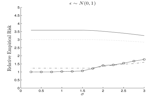
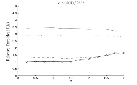
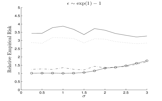
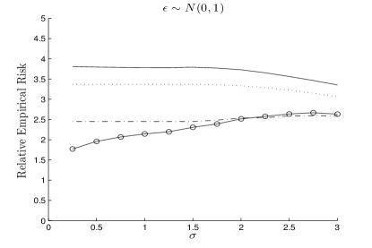
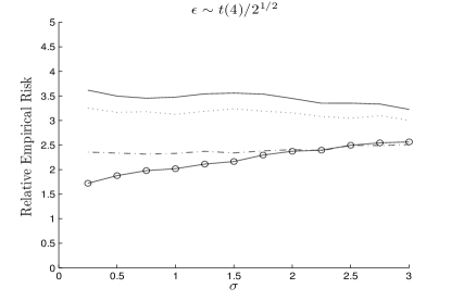
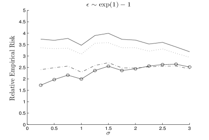
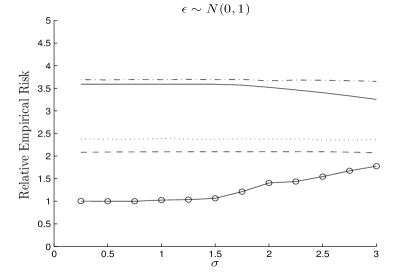
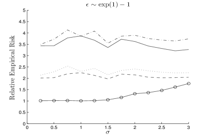
The results of computational experiments for designs a), b) and c) in Figures 3 and 3 illustrates the theoretical results indicated obtained in the paepr. That is, the performance of the non-Gaussian cases b) and c) is very similar to the Gaussian case. Moreover, as expected, higher correlation between covariates translates into larger empirical risk.
The performance of square-root lasso and post square-root lasso are relatively close to the performance of lasso and post lasso that knows . These results are in close agreement with our theoretical results, which state that the upper bounds on empirical risk for square-root lasso asymptotically approach the analogous bounds for infeasible lasso.
C.3. Comparison with feasible versions of lasso
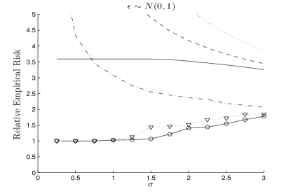
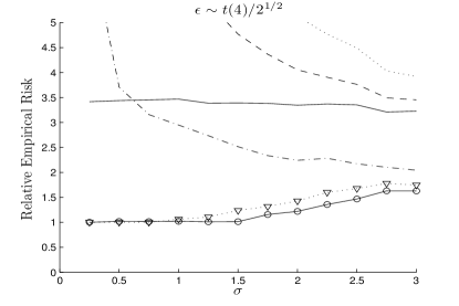
Next we focus on the Toeplitz design above to compare many traditional estimators related to lasso. More specifically we consider the following estimators: (1) oracle estimator, which is ols applied to the true minimal model (which is unknown outside the experiment), (2) infeasible lasso with known (which is unknown outside the experiment), (3) post lasso, which applies ols to the model selected by infeasible lasso, (4) square-root lasso, (5) post square-root lasso, which applies least squares to the model selected by square-root lasso, (6) 1-step feasible lasso, which is lasso with an estimate of given by the conservative upper bound where , (7) post 1-step lasso, which applies least squares to the model selected by 1-step lasso, (8) 2-step lasso, which is lasso with an estimates of given by the 1-step lasso estimator , namely , (9) post 2-step lasso, which applies least squares to the model selected by 2-step lasso, (10) cv-lasso, which is lasso with an estimate of given by K-fold cross validation, (10) post cv-lasso, which applies OLS to the model selected by K-fold lasso, (11) square-root lasso (1/2), which uses the penalty of square-root lasso multiplied by , (12) post square-root lasso (1/2), which applies least squares to the model selected by square-root lasso (1/2). We generate regressors as with the Toeplitz correlation matrix .
We focus our evaluation of the performance of an estimator on the relative average empirical risk with respect to the oracle estimator , .
Comparison of square-root lasso to cross-validation choice of

Comparison of square-root lasso to other feasible lasso methods
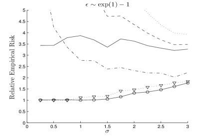
We present the results comparing square-root lasso to lasso where the penalty parameter is chosen based on -fold cross-validation procedure. We report the experiments for designs a), b) and c) in Figure 5. The first observation is that as indicated by theoretical results of the paper, the performance of the non-Gaussian cases b) and c) is very similar to the Gaussian case so we focus on the later.
We observe that cv-lasso does improve upon square-root lasso (and infeasible lasso as well) with respect to empirical risk. The cross-validation procedure selects a smaller penalty level, which reduces the bias. However, cv-lasso is uniformly dominated by a square-root lasso method with penalty scaled by 1/2. Note the computational burden of cross-validation is substantial since one needs to solve several different lasso instances. Importantly, cv-lasso does not perform well for purposes of model selection. This can be seen from the fact that post cv-lasso performs substantially worse than cv-lasso. Figure 5 also illustrates that square-root lasso performs substantially better than cv-lasso for purposes of models selection since post square-root lasso thoroughly dominates all other feasible methods considered.
Figure 6 compares other feasible lasso methods that are not as computational intense as cross-validation. The estimator with the best performance for all noise levels considered was the post square-root lasso reflecting the good model selection properties of the square-root lasso. The simple 1-step lasso with conservative estimate of does very poorly. The 2-step lasso does better, but it is still dominated by square-root lasso. The post 1-step lasso and the post 2-step lasso are also dominated by the post square-root lasso on all noise levels tested.
Appendix D Proofs of Additional Theoretical Results
Proof of Lemma 3.
Part 1. Let and for some slowly enough let for large enough. Thus,
since . To bound the first term above, by Condition SN, we have that for large enough where slowly enough. Thus, by the union bound and Lemma 7
where under condition SN, and the last inequality follows from standard bounds on , and calculations similar to those in the proof of Lemma 1 of the main text. Moreover,
since since . It follows that
by the choice of and the application of Rosenthal’s inequality.
Moreover, for sufficiently large, letting , we have
by condition SN since we have , is uniformly bounded above, , and . Thus, applying Lemma 8, noting the relation above, we have
Part 2. Let and for some slowly enough let for large enough. Thus,
By the same argument as in part 1 we have
To bound the first term above, by Condition SN, we use that for large enough where slowly enough. Thus, by the union bound and Lemma 7
where the last inequality follows from standard bounds on and calculations and calculations similar to those in the proof of Lemma 1 of the main text.
Therefore, for sufficiently large,
so that . ∎
Appendix E Omitted Proofs from the Main Text
E.1. Omitted Part of Proof of Lemma 1.
Claim in the proof of Lemma 1: For independent random variables and any , we have
It follows from
where we have , so that . Applying the second inequality of Lemma 1 of [12] for , we have
E.2. Omitted Part of Proof of Lemma 2.
To show statement (iv) of Lemma 2, it suffices to show that for any , , which follows analogously to the proof of statement (iii).
Indeed, for some constants ,
where (1) holds by the union bound; (2) holds by the application of the Rosenthal and Vonbahr-Esseen inequalities:
provided that
To verify relation (3), by Condition M and Slastnikov-Rubin-Sethuraman’s theorem on moderate deviations, we have that uniformly in for some , uniformly in and for any , , so the relation (3) holds to for for by assumption, provided is set sufficiently close to 1 so that .
When , for large we can also bound by where , , and invoking the Slastnikov’s theorem as previously, which gives
Taking the best conditions on gives the restriction:
| (38) |
Appendix F Tools Used
F.1. Rosenthal and Von Bahr-Esseen Inequalities
Lemma 4.
Let be independent zero-mean random variables, then for
This is due to [18].
Corollary 5.
Let , and consider the case of identically distributed zero-mean variables with and bounded by . Then for any
To verify the corollary, we use Rosenthal’s inequality , and the result follows by Markov inequality,
Lemma 5.
Let be independent zero-mean random variables. Then for
This result is due to [26].
Corollary 6.
Let , and consider the case of identically distributed zero-mean variables with bounded by . Then for any
The corollary follow by Markov and Vonbahr-Esseen’s inequalities,
F.2. Moderate Deviations for Sums
Let be a double sequence of row-wise independent random variables with , , ; , and as . Let
The following result is due to [21].
Lemma 6.
If for sufficiently large and some positive constant ,
where is slowly varying function monotonically growing to infinity and as , then
uniformly in the region .
Corollary 7.
If and then
uniformly in the region .
Remark. Rubin-Sethuraman derived the corollary for for fixed . Slastnikov’s result adds uniformity and relaxes the moment assumption.
F.3. Moderate Deviations for Self-Normalizing Sums
We shall be using the following two technical results. The first follows from Theorem 7.4 in [7] which is based on [9].
Lemma 7.
Let be the triangular array of independent non-identically distributed zero-mean random variables. Suppose
Then there is a universal constant such that uniformly on , the quantities
obey
The second follows from the proof of Lemma 10 given in the working paper “Pivotal Estimation of Nonparametric Functions via Square-root Lasso”, arXiv 1105.1475v2, by the authors, which is based on symmetrization arguments.
Lemma 8.
Let () be independent identically distributed random variables such that and for . Conditional on , with probability
References
- [1] A. Beck and M. Teboulle. A fast iterative shrinkage-thresholding algorithm for linear inverse problems. SIAM J. Imaging Sciences, 2(1):183–202, 2009.
- [2] Stephen Becker, Emmanuel Candès, and Michael Grant. Templates for convex cone problems with applications to sparse signal recovery. ArXiv, 2010.
- [3] A. Belloni and V. Chernozhukov. -penalized quantile regression for high dimensional sparse models. Ann. Statist., 39(1):82–130, 2011.
- [4] P. J. Bickel, Y. Ritov, and A. B. Tsybakov. Simultaneous analysis of Lasso and Dantzig selector. Ann. Statist., 37(4):1705–1732, 2009.
- [5] F. Bunea, A. B. Tsybakov, and M. H. Wegkamp. Aggregation for Gaussian regression. Ann. Statist., 35(4):1674–1697, 2007.
- [6] E. Candès and T. Tao. The Dantzig selector: statistical estimation when is much larger than . Ann. Statist., 35(6):2313–2351, 2007.
- [7] V. H. de la Peña, T. L. Lai, and Q.-M. Shao. Self-Normalized Processes. Springer, 2009.
- [8] J. Huang, J. L. Horowitz, and S. Ma. Asymptotic properties of bridge estimators in sparse high-dimensional regression models. Ann. Statist., 36(2):587 613, 2008.
- [9] B. Y. Jing, Q. M. Shao, and Q. Y. Wang. Self-normalized Cramér type large deviations for independent random variables. Ann. Probab., 31:2167–2215, 2003.
- [10] V. Koltchinskii. Sparsity in penalized empirical risk minimization. Ann. Inst. H. Poincar Probab. Statist., 45(1):7–57, 2009.
- [11] G. Lan, Z. Lu, and R. D. C. Monteiro. Primal-dual first-order methods with interation-complexity for cone programming. Mathematical Programming, (126):1–29, 2011.
- [12] B. Laurent and P. Massart. Adaptive estimation of a quadratic functional by model selection. Ann. Statist., 28(5):1302–1338, 2000.
- [13] N. Meinshausen and B. Yu. Lasso-type recovery of sparse representations for high-dimensional data. Ann. Statist., 37(1):2246–2270, 2009.
- [14] Y. Nesterov. Smooth minimization of non-smooth functions, mathematical programming. Mathematical Programming, 103(1):127–152, 2005.
- [15] Y. Nesterov. Dual extrapolation and its applications to solving variational inequalities and related problems. Mathematical Programming, 109(2-3):319–344, 2007.
- [16] Y. Nesterov and A Nemirovskii. Interior-Point Polynomial Algorithms in Convex Programming. Society for Industrial and Applied Mathematics (SIAM), Philadelphia, 1993.
- [17] J. Renegar. A Mathematical View of Interior-Point Methods in Convex Optimization. Society for Industrial and Applied Mathematics (SIAM), Philadelphia, 2001.
- [18] H. P. Rosenthal. On the subspaces of spanned by sequences of independent random variables. Israel J. Math., 9:273 –303, 1970.
- [19] Herman Rubin and J. Sethuraman. Probabilities of moderatie deviations. Sankhyā Ser. A, 27:325–346, 1965.
- [20] Mark Rudelson and Roman Vershynin. On sparse reconstruction from Fourier and Gaussian measurements. Comm. Pure and Applied Mathematics, 61:1025 –1045, 2008.
- [21] A. D. Slastnikov. Limit theorems for moderate deviation probabilities. Theory of Probability and its Applications, 23:322–340, 1979.
- [22] A. D. Slastnikov. Large deviations for sums of nonidentically distributed random variables. Teor. Veroyatnost. i Primenen., 27(1):36–46, 1982.
- [23] R. Tibshirani. Regression shrinkage and selection via the lasso. J. Roy. Statist. Soc. Ser. B, 58:267–288, 1996.
- [24] K. C. Toh, M. J. Todd, and R. H. Tutuncu. On the implementation and usage of sdpt3 – a matlab software package for semidefinite-quadratic-linear programming, version 4.0. Handbook of Semidefinite, Cone and Polynomial Optimization: Theory, Algorithms, Software and Applications, Edited by M. Anjos and J.B. Lasserre, June 2010.
- [25] S. A. van de Geer. High-dimensional generalized linear models and the lasso. Ann. Statist., 36(2):614–645, 2008.
- [26] Bengt von Bahr and Carl-Gustav Esseen. Inequalities for the rth absolute moment of a sum of random variables, . Ann. Math. Statist, 36:299–303, 1965.
- [27] M. Wainwright. Sharp thresholds for noisy and high-dimensional recovery of sparsity using -constrained quadratic programming (lasso). IEEE Transactions on Information Theory, 55:2183–2202, May 2009.
- [28] C.-H. Zhang and J. Huang. The sparsity and bias of the lasso selection in high-dimensional linear regression. Ann. Statist., 36(4):1567–1594, 2008.
- [29] Tong Zhang. On the consistency of feature selection using greedy least squares regression. J. Machine Learning Research, 10:555–568, 2009.
- [30] P. Zhao and B. Yu. On model selection consistency of lasso. J. Machine Learning Research, 7:2541–2567, Nov. 2006.