Statistically Stable Estimates of Variance in Radioastronomical Observations as Tools for RFI Mitigation

Abstract

A selection of statistically stable (robust) algorithms for data variance calculating has been made. Their properties have been analyzed via computer simulation. These algorithms would be useful if adopted in radio astronomy observations in the presence of strong sporadic radio frequency interference (RFI). Several observational results have been presented here to demonstrate the effectiveness of these algorithms in RFI mitigation.

1 Introduction

Cosmical radio emissions received by radio telescopes are noise-like signals which are characterized by a normal (Gaussian) probability distribution function ${\cal N}(0,\sigma_{sig})$, i.e., with zero mean and variance $\sigma_{sig}^{2}$. Background radio emission and radio receivers also produce normal noise ${\cal N}(0,\sigma_{sys})$. Given a large number of n samples $x_{i},i=0..n$ of normally distributed data with zero mean, a classical statistical procedure for the estimation of variance $\sigma^{2}$ is

$$\widehat{\sigma^{2}_{n}}=\frac{1}{n}\sum_{i=1}^{n}x_{i}^{2}$$ (1)

The time-honoured estimate (1) may be obtained by using the Maximum Likelihood method (van der Waerden, 1969) and is a minimum variance unbiased estimate. Traditional radiometrical techniques implement this procedure in analogue or digital form in conventional radiometers: the estimate of $\widehat{\sigma_{sig}^{2}+\sigma_{sys}^{2}}$ is obtained after square-law detection and low-pass filtering (averaging) (Rohlfs & Wilson, 2003). This statistical inference is based upon an essential assumption about the probability distribution of the data “signal noise + systen noise”: the distribution must be normal. As in many cases in applied statistics this assumption is not always valid for radio astronomy. Most of the data may correspond to the model with an assumed normal distribution, but there are also a number of outliers, atypical data which stand out from the bulk of the data. As a result there is an “approximately” normal distribution that gives rise to outliers, i.e., the distribution has a normal shape in the central region but has tails that are heavier than those of a normal distribution. If such approximate normality were to hold, the results of using a normal distribution theory will nevertheless not hold approximately. In the presence of heavy tails the estimate (1) based on the maximum likelihood principle is no longer the best and may have unacceptably low statistical efficiency (large variance) and very large bias. These phenomena in applied statistics have been well known from the time of Gauss, Newcomb and Eddington.

Radio frequency interference (RFI) creates a situation in radio astronomy where such outliers arise (Fridman & Baan, 2001; Kesteven, 2007). Industry, ground and satellite communications, ground and airborne radar, power lines, radio and TV stations, etc. produce all kinds of additional noise which penetrate into extremely sensitive radio astronomy receivers. Radio observatory computers are themselves often the sources of RFI. Many authors demonstrated the effectiveness of different RFI mitigation methods (Ellingson & Hampson, 2003; Baan, Fridman & Millenaar, 2004; Fisher et al., 2005; Mitchell, Robertson & Sault, 2005; Poulsen, Jeffs & Warnick, 2005; Zhang et al., 2005; Kesteven, 2007) in observations with single dishes and radio interferometers. Adaptive noise cancellation (ANC) with reference antenna was described in (Barnbaum & Bradley, 1998). Post detector and post correlation processing using reference antennas was suggested in (Briggs,Bell & Kesteven, 2000). Higher order statistics (HOS) analysis was proposed in (Fridman, 2001). Principal results were achieved with blanking and reference antennas. The high expectations of new projects (LOFAR, ATA, SKA) are based on the implementation of spatial processing - nulling in the direction of RFI. But very often RFI do not obey the model assumptions which guarantee the success of this kind of processing. They are variable, sporadic and are not fully coherent at the sites of multi-element systems (Thompson, 2003; Jeffs, Li & Warnick, 2005).

In this paper a new view on blanking is proposed based on statistical methods granting stable estimates of variance in the presence of outliers. These methods would be useful in radio astronomy RFI mitigation, including real-time processing. The aim of this paper is to compile a selection of methods of stable variance estimates suitable for RFI mitigation and to study their properties via computer simulation. Some examples obtained during real observations are also given.

The typical appearances of RFI is of strong impulse-like bursts in both temporal and spectral domains. They behave as outliers in the data with normal distribution and the data received may be characterized by the contaminated normal distribution

$$F(x)=(1-\epsilon){\cal N}(0,\sigma_{sys})+\epsilon F_{RFI}(x),$$ (2)

where ${\cal N}(0,\sigma_{sys})$ is the “clean” probability distribution, $F_{RFI}(x)$ is the usually unknown distribution of RFI, $\epsilon$ characterizes the fraction of $F_{RFI}(x)$ in the total $F(x),0<\epsilon<1$. The theory of robustness pioneered by (Tukey, 1960; Huber, 1964; Hampel, 1971) gives recommendations on obtaining statistically stable estimates of parameters in the situation similar to (2). The estimate is called statistically stable (robust) if slight changes in distribution have a relatively small effect on its value, or, in other words, robustness means insensitivity of a statitical procedure to small deviations from assumptions about the normality of data’s distribution.

Several approaches to developing robust estimates exist: $M$-estimates based on a generalized maximum likelihood (Huber, 2004), $L$-estimates based on order statistics (David & Nagaraja, 2003), $R$-estimates based on ranks (Hettmansbperger, 1984) and estimates based on nonparametrical statistics (Sheskin, 2000).

2 Stable estimates of variance

A selection of stable (robust) estimates of variance will be described in this section. There are different ways of judging the stability of an estimate. Given a distribution $F(x)$ and a population $X$ representing this distribution, an estimate $T(X,F)$ is the functional depending on $F(x)$. If this estimate is relatively unaffected by small changes in $F$, i. e., the functional is continuous with respect to $F$, then the estimate is said to have qualitative robustness. For a distribution $F(x)$ contaminated by a distribution $G(x)$ with probability $\epsilon$

$$F_{\epsilon}(x)=(1-\epsilon)F(x)+\epsilon G(x)$$ (3)

the influence function (Hampel et al., 1986) $IF(T,F)$ is widely used in theoretical analysis

$$IF(x)=\lim_{\epsilon\rightarrow 0}\frac{T(F_{x,\epsilon})-T(F_{x})}{\epsilon}$$ (4)

The $IF(T,F)$ is the relative influence of x on $T(F)$ having the value $x$ with probability $\epsilon$. The estimate $T(F)$ is said to have infinitesimal robustness if $IF(x)$ is bounded. The $IF$ of classical both arithmetical mean and variance are not bounded. A simple finite-sample version of $IF$ called empirical influence function (or sensitivity function) exists. It is constructed in the following way. Suppose there is an estimate $T_{n-1}$ of a sample $(x_{1},...,x_{n-1})$. A new $n-th$ sample $x$ is added and $T_{n}(x_{1},...,x_{n-1},x)$ is considered as a function of x. For the estimate (1) the sensitivity function is

$$IF(x)=\frac{x^{2}-\widehat{\sigma^{2}_{n}}}{n+1}$$ (5)

Another useful characteristic of robustness is the breakdown point: the minimum value of $\epsilon$ for which an estimate goes to infinity as $x$ grows. The breakdown point of conventional mean and variance is 0. The breakdown point of median is 0.5, i.e., up to 50% of data may be outliers and they do not alter the correct value of the median.

Taking into consideration our practical goal to use estimates of variance in observations, two measures of stability will be exploited for the following statistical procedures.

1. The relative empirical influence function with the following modification: for a sample length $N$ the number of additional outliers with an amplitude $X_{RFI}$ will be $M=[\epsilon N]$, where $[q]$ means the greatest integer part of $q$. The estimate calculated for a contaminated sample is compared with the estimate correspondimg to a “clean” sample:

$$REIF(\epsilon x)=\frac{T_{N+M}(F_{x,\epsilon})-T_{N+M}(F_{x,\epsilon=0})}{T_{N+M}(F_{x,\epsilon=0})}.$$ (6)

The relative empirical influence function will be calculated during computer simulation for the estimates described below.

2. Stability against outliers is achieved at the expense of the effectiveness of an estimate. In the absence of outliers the standard deviation of a robustly estimated variance is, as a rule, larger than that of a simple estimate (1). To characterize this loss the parameter $LOSS$ will be used:

$$LOSS=SNR_{T_{N}}/SNR0,$$ (7)

$$SNR_{T_{N}}=\frac{\widehat{T_{N}(\sigma+\Delta\sigma)}-\widehat{T_{N}(\sigma)}}{rms[\widehat{T_{N}(\sigma)}]},$$

$$SNR0=\frac{\widehat{T0_{N}(\sigma+\Delta\sigma)}-\widehat{T0_{N}(\sigma)}}{rms[\widehat{T0_{N}(\sigma)}]}.$$

For a small increase of $\Delta\sigma<<\sigma$ two signal-to-noise ratios $SNR$ are compared: $SNR_{T_{N}}$ of a given estimate of variance $\widehat{T_{N}(\sigma)}$ and $SNR0$ of the estimate (1) with the best potential effectiveness.

The relative empirical influence function and loss are calculated via computer simulations ($\sigma=1,n=10^{5}$) for the estimates presented below.

2.1 Variance of the trimmed data

Let $x_{1},....,x_{n}$ be a random sample and let $x_{(1)}\leq x_{(2)}\leq...\leq x_{(n)}$ be the observations sorted in ascending order. The $ith$ largest value $x_{(i)}$ is called the $ith$ order statistic. Let $\gamma$ denote the chosen amount of trimming, $0\leq\gamma\leq 0.5$ and $k=[\gamma n]$. The sample trimmed variance is computed by removing the $k$ largest and $k$ smallest data and using the values that remain:

$$T_{1}=\frac{K_{trim}}{N-2k}\sum_{n=k}^{N-k}(x_{n}-\widehat{\mu}_{trim})^{2}$$ (8)

$$\widehat{\mu}_{trim}=\frac{1}{N-2k}\sum_{n=k}^{N-k}x_{n},$$

where $\mu_{trim}$ is the sample mean of the trimmed data. Trimming lessens the variance of data and the coefficient $K_{trim}$ makes $T_{1}$ the consistent estimator for data with normal distribution. Table 1 gives the values of $K_{trim}$ for different $\gamma$.

Table 1: Consistency factor and $LOSS$ as functions of $\gamma$ for trimming

$\gamma$	0.005	0.01	0.025	0.05	0.1
$K_{trim}$	1.085	1.147	1.32	1.6	2.28
$LOSS$	0.98	0.95	0.90	0.86	0.83

The third row in this table gives the values of $LOSS$ for different $\gamma$.
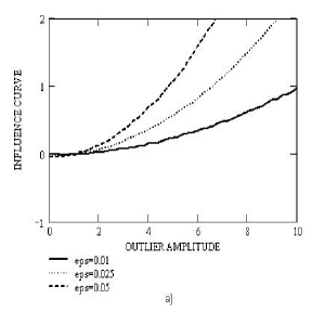
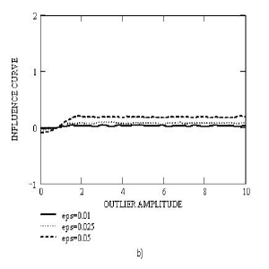
Fig. 1 shows the relative empirical influence functions for untrimmed data (Fig. 1a) and for the variances computed for trimmed data with $\gamma=0.05$ (Fig. 1b). The parameter $\epsilon$ (“eps”) indicates the percentage of outliers in the total volume of data.

2.2 Winsorized sample variance

A sample $x_{1},....,x_{n}$ is sorted in ascending order. For the chosen $0\leq\gamma\leq 0.5$ and $k=[\gamma n]$ winsorization of the sorted data consists of setting

$$W_{i}=\left\{\begin{array}[]{lcl}x_{(k+1)},&if&x_{(i)}\leq x_{(k+1)}\\ x_{(i)},&if&x_{(k+1)}<x_{(i)}<x_{(n-k)}\\ x_{(n-k)},&if&x_{(i)}\geq x_{(n-k})\\ \end{array}\right.$$ (9)

The winsorized sample mean is $\widehat{\mu_{w}}=\frac{1}{n}\sum_{i=1}^{n}W_{i}$ and the winsorized sample variance is

$$T_{2}=\frac{1}{n-1}\sum_{i=1}^{n}(W_{i}-\widehat{\mu_{w}})^{2}$$ (10)

Table 2 gives values of the consistency factor $K_{winsor}$ for different $\gamma$.

Table 2: Consistency factor and $LOSS$ as functions of $\gamma$ for winsorization

$\gamma$	0.005	0.01	0.025	0.05	0.1
$K_{winsor}$	1.019	1.041	1.103	1.227	1.54
$LOSS$	0.99	0.98	0.96	0.88	0.82

The third row of this table gives the values of $LOSS$ for different $\gamma$.
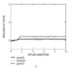
Fig. 1c shows the relative empirical influence functions for the variances computed for winsorized data with $\gamma=0.1$. The parameter $\epsilon$ (“eps”) indicates the percentage of outliers in the total volume of data.

2.3 Median absolute deviation

This estimate for sorted data $x_{(1)}\leq x_{(2)}\leq...\leq x_{(n)}$ is defined by

$$T_{3}=1.483\times med_{1\leq i\leq n}\{\left|x_{i}-med(x_{i})\right|\},$$ (11)

where

$$\left.\begin{array}[]{lll}med=&0.5(x_{(m)}+x_{(m+1)}),&n=2m,\\ med=&x_{(m+1)},&n=2m+1\\ \end{array}\right.$$

The breakdown point for this estimate is 0.5, i.e., almost half the data may be contaminated by outliers. But the effectiveness of $T_{3}$ is much lower than for the $T_{1}$ and $T_{2}$: the $LOSS=0.6$.

2.4 Interquartile range

This estimate is defined by

$$T_{4}=[(x_{1-q}-x_{q})/1.35]^{2},$$ (12)

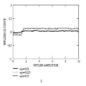
where $q=0.25$ and for distribution $\cal{P}$ $x_{q}$ satisfies $\cal{P}$$(x\leq x_{q})=q$. The breakdown point for $T_{4}$ is 0.25 and the $LOSS=0.6$. Fig. 1i shows the relative empirical influence functions for the variances computed with $T_{4}$.

2.5 Median of pairwise averaged squares

This estimate is motivated by the Hodges-Lehmann estimate of location

$$\widehat{\mu_{n}}=med(\frac{x_{i}+x_{j}}{2},1\leq i\leq j\leq n),$$

which for variance is

$$T_{5}=1.483\times med_{1\leq i\leq jn}[(x_{i}^{2}+x_{j}^{2})/2]$$ (13)

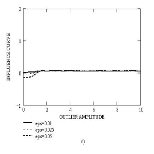
Fig. 1d shows the relative empirical influence functions for the variances computed with $T_{5}$ . The parameter $\epsilon$ (“eps”) indicates the percentage of outliers in the total volume of data. The $LOSS$ for $T_{5}$ is 0.78.

2.6 $Qn$ estimate

This estimate is proposed in (Rousseuw & Croux, 1993) and requires fewer operations than $T_{5}$, but is quite effective. It combines the ideas of the Hodges-Lehmann estimate and the Gini estimate (Kendal & Stuart, 1967):

$$T_{6}=2.2219\{\left|x_{i}-x_{j}\right|,i\leq j\}_{(k)},$$ (14)

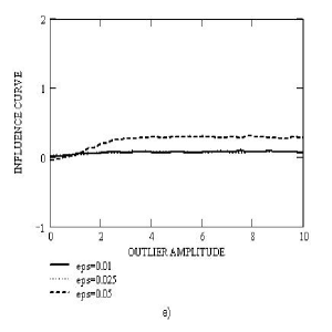
where $k={h\choose 2}$ and $h=[n/2]+1,k\approx{n\choose 2}/4$. This estimate is the $kth$ order statistic of the ${n\choose 2}$ interpoint distances. Fig. 1e shows the relative empirical influence functions for variances computed with $T_{6}$. The $LOSS=0.88$.

2.7 Biweight variance

First the following auxiliary values are calculated

$$Y_{i}=\frac{x_{i}-M}{9\times MAD},$$

where $M$ and $MAD$ are the median mean and median absolute deviation, respectively. Then the coefficients are defined as

$$a_{i}=\left\{\begin{array}[]{ll}1,&if\left|Y_{i}\right|<1\\ 0,&if\left|Y_{i}\right|\geq 1\end{array}\right.$$

in which case the estimate is

$$T_{7}=\frac{\sqrt{\sum_{i=1}^{n}a_{i}(x_{i}-M)^{2}(1-Y_{i})^{4}}}{\left|\sum_{i=1}^{n}a_{i}(1-Y_{i}^{2})(1-5Y_{i}^{2})\right|}$$ (15)

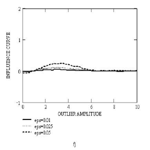
Fig. 1f shows the relative empirical influence functions for variances computed with $T_{7}$. The $LOSS=0.92$.

2.8 Bend Midvariance

This estimate of variance is described in (Wilcox, 2004). Set $\beta=0.1$ and $m=[(1-\beta)n+0.5]$. Let $W_{i}=\left|x_{i}-M\right|,i=1,...n$, and $W_{(i)}$ are these numbers sorted in ascending order, M is the median mean of data $x$. Then the estimate of $1-\beta$ quantile of the distribution of $W_{(i)}$ is $\widehat{\omega_{\beta}}=W_{(m)}$. Now set

$$Y_{i}=\frac{x_{i}-M}{\widehat{\omega_{\beta}}}$$

and

$$a_{i}=\left\{\begin{array}[]{ll}1,&if\left|Y_{i}\right|<1\\ 0,&if\left|Y_{i}\right|\geq 1\end{array}\right.$$

in which case the bend midvariance is

$$T_{8}=\frac{\omega_{\beta}^{2}\sum_{i=1}^{n}\{(\psi(Y_{i})\}^{2}}{(\sum_{i=1}^{n}a_{i})^{2}}$$ (16)

where

$$\psi(t)=\max[-1,\min(1,t)].$$

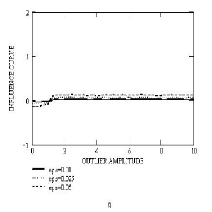
Fig. 1g shows the relative empirical influence functions for variances computed with $T_{8}$. The $LOSS=0.96$.

2.9 Estimate with exponential weighting

This estimate is described in (Shurygin, 2000). Mean is estimated as a solution of the equation

$$\widehat{\mu_{r}}:\hskip 14.22636pt\sum_{i=1}^{n}(x_{i}-\widehat{\mu_{r}})e^{-q_{i}/4}=0$$ (17)

and variance is defined as a solution of the equation

$$T_{9}=\sigma_{r}^{2}:\hskip 14.22636pt\sum_{i=1}^{n}[(x_{i}-\widehat{\mu_{r}})^{2}/\sigma_{r}^{2}-2/3]e^{-q_{i}/4}=0,$$ (18)

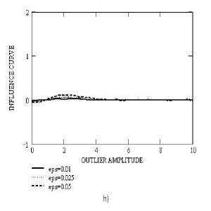
where $q_{i}=(x_{i}-\widehat{\mu_{r}})^{2}/\widehat{\sigma^{2}}$. Fig. 1h shows the relative empirical influence functions for variances computed with $T_{9}$. The $LOSS=0.98$.

D. A. Lax performed a Monte Carlo study of more than 150 variance estimators. Seventeen of these estimators were selected as being either promising or commonly used (Lax, 1985). The results of our computer simulation are in agreement with this test (Lax, 1985), especially concerning the high efficiency of estimate $T_{1}$ and $T_{7}$ and the low efficiency of $T_{3}$.

The choice of a particular estimate depends on the type and intensity of RFI, the type of observations and the method of implementation (hardware or software). $T_{8}$ and $T_{9}$ are the best estimates from the point of view of $LOSS$. $T_{3}$ and $T_{5}$ remove outliers in a most effective way (high value of the breakdown point). Number sorting and permutations of pairwise measurements which are necessary in several algorithms require more computational time and computer memory.

3 Computer simulations

This section presents computer simulations of RFI mitigation using algorithms which were employed in observations (Section 4). Two estimators from the the previous section have been chosen: winsorization and exponential weighting. The reasons for this choice are as follows.

All algorithms described in Section 2 give estimates of variance, i.e., they work as total power detectors (TPD) in radiotechnical terminology. They can be applied in single dish observations both in continuum and in spectral observations. In the same manner they can substitute for TPDs which are already installed in existing radio telescopes. Nowadays it is practically impossible for technical and organizational reasons.In future radio relescopes may be equipped with some RFI mitigation techniques and these variance estimators could then be implemented in hardware or software shape. But at the present time any experiment with RFI mitigation at existing ratio telescopes must take the technical constraints of implementation into account. Therefore only those estimators from Section 2 were chosen which could provide not only estimates of variance but also “clean” data which could be applied further to TPD or to the correlator already in use in a radio telescope backend.

3.1 Winsorization followed by total power detectors

Winsorization with the parameter $\gamma=0.05$ was chosen mainly because impulse-like RFI in the temporal domain was predominant during observations made at Effelsberg presented in Fig. 8. It was strong and sparse. The percentage of RFI in the whole volume of data was not large $(<5\%)$. Both winsorization and trimming can provide raw data without outliers but trimming inconveniently reduces the number of samples because of this implementation problem: “timing” is distorted, i. e., there are gaps (not zeros) in the presumed unbroken flow of data and the radio telescope backend has no information about the location of these gaps. The problem is easily solved in software during simulations but may be critical in real observations. Winsorization unlike trimming preserves the total number of samples.

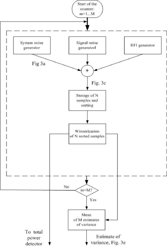
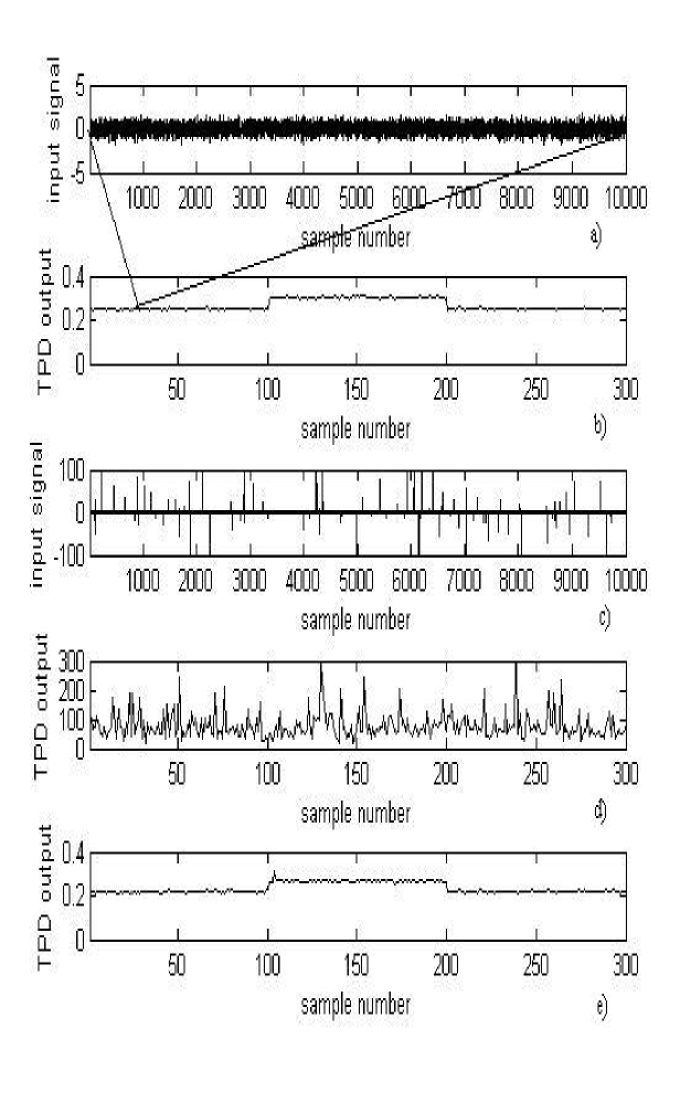
The block diagram of computer simulation presented in Fig. 2 shows the structure of the algorithm using winsorization. The input signal is the mixture of three signals: system noise with normal distribution ($\sigma=0.5$), signal noise, also with normal distribution ($\sigma=0.05$) and impulse-like interference imitating RFI. The signal noise is switched “on” and “off” emulating “on-source” or “off-source” position of the antenna main beam, respectively. Poisson distribution ($\lambda=0.004$) governs the appearance of RFI and the lognormal distribution (mean=12, standard deviation=6) determines the random amplitudes of impulses. Input signal samples are stored in the buffer and sorted to create order statistics. The length of these statistics is equal to $N=100$. The winsorization block provides both variance estimates for each of the $N$ samples and also the winsorized samples which are applied to the external TPD (as in observations presented in subsection 4. 1). The loop with $M=100$ cycles corresponds to post-detector averaging: the estimates of variance after the winsorization block are accumulated during $M$ cycles and the mean calculated for these $M$ cycles represents the simulation result.

Fig. 3 shows the results of computer simulations :
a) input noise with normal distribution, $\mu=0.0,\sigma=0.5$, no interference; b) total power detector output, each point in this figure corresponds to squaring and averaging of $N\times M=10^{4}$ samples in figure a); there are two steps, “up” at point $\#100$ and “down” at point $\#200$ corresponding to the increase of $\sigma$ from value $0.5$ to the value $\sigma+\Delta\sigma,\Delta\sigma=0.05$ ( “on-source” and “off-source” position of antenna beam);
c) interferences in the form of random impulses are added to the noise a);
d) total power detector output with the input signal c);
e) total power detector output with the input signal c) and preliminary winsorization. The difference between the scales in the vertical axes in d) and e) demonstrates the effect of interference mitigation.

3.2 Exponential weighting

Exponential weighting also provides not only estimates of variance but data with suppressed outliers. This estimator is also of superior effectiveness. And unlike winsorization, it does not sort input data. The influence of sorting on phase information can be detrimental to radiointerferometic and pulsar (de-dispersion procedure) observations. Impulse-like RFI in the frequency domain was prevalent during the pulsar and image synthesis observations at WSRT (subsection 4. 2 and 4. 3). It is to demonstrate exponential weighting in the frequency domain which is the aim of this computer simulation.

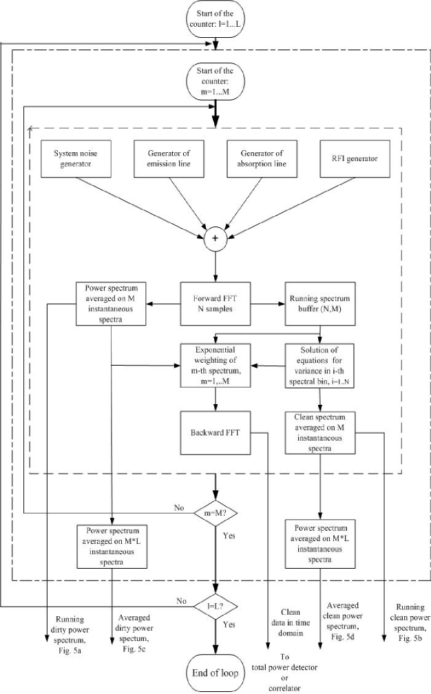
The block diagram presented in Fig. 4 shows the structure of the algorithm using exponential weighting in the spectral domain. The input signal is a mixture of four signals: system noise with normal distribution ($\sigma=1.0$) filtered to emulate the WSRT backend low-pass filters; two noise-like signals with normal distribution imitating emission and absorption spectral lines, respectively, and interference waveforms. A randomly phase-modulated sinusoidal carrier is used as the RFI signal, the index of modulation is equal to $\pi/2$ (binary phase modulation). Poisson distribution ($\lambda=0.3$) determines the moments of phase jumps.

There are two loops in the algorithm: the inner loop ($m=1,..M$) which is responisble for the storage of $M$ instantaneous spectra of the input signal for RFI mitigation processing, and the outer loop ($l=1,..L$) which repeats consecutively $L$ identical stages of processing inside the inner loop, showing the dynamics of the running spectrum. Interference is intermittently switched “on” and “off” inside the inner loop, the percentage in the total averaging interval is less than $7\%$.

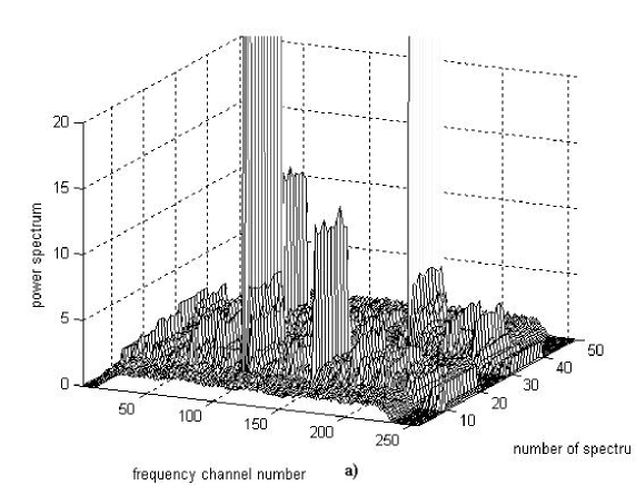
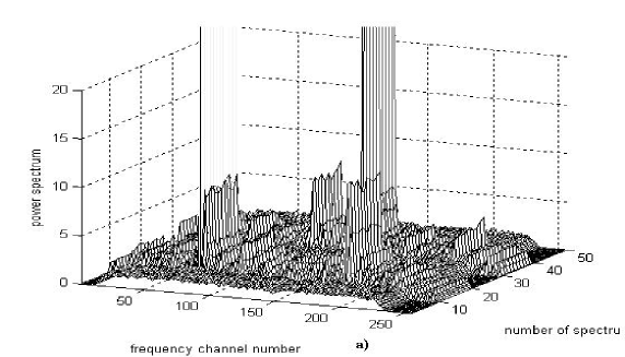
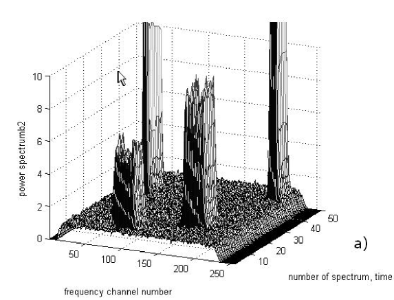
$N$ samples of the input signal are Fourier-transformed with forward FFT, $N=512$. The inner loop with the counter ($m=1,..M$) provides $M$ complex spectra (each having a length equal to $N$) which are stored in the buffer. So there are two sets (real and imaginary) of data in the buffer numbered as $m=1,..M$ for each of the $N=512$ spectral channels. $L$ power spectra of the input signal averaged on $M$ instantaneous spectra are calculated in the outer loop ($l=1,..L$). Fig. 5a shows the three-dimensional time-frequency presentation of the sequence of $L=50$ averaged “dirty” spectra.

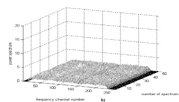
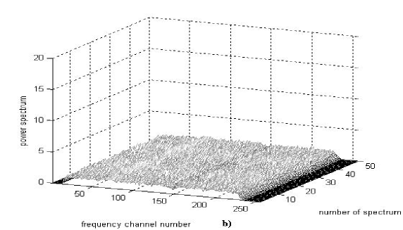
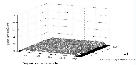
Equation (18) is solved separately for each of $2\times N$ real and imaginary sets of data providing estimates of $\widehat{\sigma^{2}_{M,real}(i)}$ and $\widehat{\sigma^{2}_{M,imag}(i)}$ - variances in $i=1,..N$ spectral channels calculated using $M$ samples of real and imaginary components of the instantaneous spectra. Random values in the real and imaginary part of the instantaneous spectrum are independent, so the sum of these estimates in each spectral channel gives the total estimated power spectrum for each spectral channel. This “clean” power spectrum is represented in Fig. 5b for $L=50$ time intervals. In real observations each of $l-th$ time interval is equal to $N\times M\times\Delta t$ seconds, where $\Delta t=1/2\Delta f$ is the input signal sample interval, $\Delta f$ is the bandwidth of the input signal.
In applications it is practical to find the solution to (18) when $\mu_{r}=0$ using the approach of stochastic approximation:

$$\widehat{\sigma_{m}}=\widehat{\sigma_{m-1}}+\frac{1}{m}\sum_{k=1}^{m}(\frac{x_{k}^{2}}{\widehat{\sigma_{m-1}}}-\frac{3}{5})\exp(-\frac{x_{k}^{2}}{3\widehat{\sigma_{m-1}}}),$$ (19)

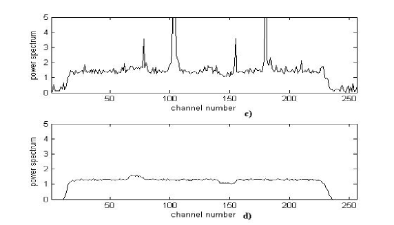
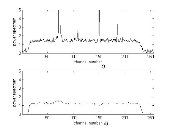
$m=1,..M$. Fig. 5c and 5d show the result of averaging $L$ spectra in Fig. 5a and 5b for the “dirty” and “clean”power spectra, respectively. The frequencies of interferences do not coincide with the frequencies of spectral lines . It can therefore be seen that the components with normal distribution (system noise and spectral lines) are untouched by this RFI mitigation procedure. The sequence of pictures in Fig. 6 similar to Fig. 5 demonstrate the result of computer simulation when the frequencies of interferences coincide with the frequencies of spectral lines . In this case we again see that the restoration of the spectra is satisfactory.

Figures 5 and 6 demonstrate how the algorithm works with spectra. However experimental constraints did not require the provision of estimates of variance or power spectrum but did required the “clean” signal in the temporal domain similar to the input signal (the level of the signal, the bandwidth). Therefore running estimates of “clean” and “dirty” power spectra are used for exponential weighting of the running complex instantaneous spectra: each complex value of an instantaneous spectrum being multiplied by $exp(-P(i)/3\widehat{\sigma^{2}(i)})$, where $P(i),i=1,..N$ is the input spectral variance (power spectrum) in the channel $i$, $\widehat{\sigma^{2}(i)}$ is the estimate of the “quiescent” power spectrum in the channel $i$ found from Eq. (18). A corresponding delay must be introduced because of the time required to calculate all $\widehat{\sigma^{2}(i)}$. Then, after the backward FFT, the signals in the temporal domain can be applied to TPDs or correlators. This auxiliary output was used to supply the “clean” raw data in the observations described in Sections 4. 2 and 4. 3.

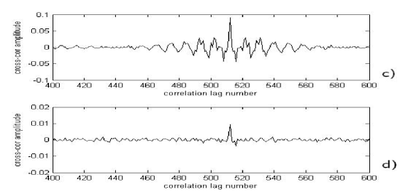
Figure 7 shows the impact of RFI mitigation on cross-correlation (radiointerferometric observations). The algorithm in the block diagram shown in Fig. 4 was applied to two signals with the additional coherent Gaussian component ($\sigma_{s}=0.1$) emulating the noise from a radio source received at both sites of the radio interferometer. Sporadic interference with the duty cycle equal to $0.2$ was generated as frequency-modulated carrier and was identical at both sites which is the worst case scenario: $100\%$ correlated RFI. In reality the impact of RFI in radio interferometers is considerably reduced due to fringe stopping and delay tracking procedures (Thompson, 1982).

Figures 7a and 7b demonstrate three-dimensional time-frequency presentations of the input “dirty” and “clean” power spectra on one site, respectively. Deep “troughs” can appear in the spectrum in Fig. 7b at the places of interferences due to the exponential effect of weighting: when interference is strong the algorithm works similarly to the “thresholding and blanking” algorithm but more smoothly and without the a priori knowledge necessary for the positioning of the threshold level. Figures 7c and 7d give the averaged normalized cross-correlation functions corresponding to Fig. 7a and 7b, without and with RFI mitigation, respectively. The central parts of the cross-correlation functions between channels $\#400$ and $\#600$ are shown. The scale of the vertical axe in Fig. 7c is significantly larger than that in Fig. 7d thus showing strong excessive cross-correlation due to RFI.

It is necessary to add two further comments here for the purposes of discussion.

1. The estimators of variance described in Section 2 and those tested in Section 3 are essentially nonlinear procedures. For example, one can, at least theoretically, imagine a huge outlier which renders the conventional estimator (1) completely non-functional whereas these estimators work perfectly. Radioastronomers often ask what is the value of RFI suppression (usually in dB) when an RFI mitigation algorithm is applied? Example in Fig. 3 demonstrates that it is not always possible to answer this question correctly. The larger the outlier’s amplitudes the more effectively they are deleted. If the amplitudes of impulses in Fig. 3c are 10 times larger the result in Fig. 3e will be the same or even slightly improved. This is also valid for the “thresholding and blanking” algorithm which has been succesfully used in several articles on RFI mitigation. That is why it is better to judge an RFI mitigation procedure in each paticular case in a combined manner, that is looking at the “signal-of-interest” distortions by both the RFI residuals and the procedure itself.

2. The estimators of Section 2 are intended for applications when sporadic, impulse-like interference disturbs observations. However interference is often continuous, persistent and practically constant during the averaging interval. For example, for $M=100,N=512,\Delta f=20MHz$ this interval is equal to $1.28\times 10^{-3}$ sec which is rather a short interval for several RFI to change their amplitudes. The estimators of Section 2 will not yield any benefits in this case. But the same fact that RFI is quasi-constant at a reasonably chosen averaging interval can help to decouple the Gaussian component with a “quiescent” value of $\sigma$ and RFI with ease. A simple procedure can do this. The power spectrum after FFT is usually calculated as

$$P(f)=1/M\sum_{m=1}^{M}\{Re[s(f)_{m}]^{2}+Im[s(f)_{m}]^{2}\}$$ (20)

The sums of RFI and “useful” Gaussian noise in each spectral channel are squared and averaged. Strong RFI dominates in this case over the noise. Another algorithm is proposed here: to separately estimate the variances of real and imaginary parts of the spectrum and then add them to obtain the total variance in each spectral channel, i.e., the power spectrum sought. The variances of real and imaginary parts of the complex spectrum must be calculated taking into consideration that the mean value now is no longer equal to zero because of the presence of RFI. So the general formula for sample variance must be applied: for a random value $x$, the sample variance is $var(x)=$$\widehat{\sigma_{x}^{2}}=1/M\sum_{m=1}^{M}(x_{m}-\widehat{x})^{2}$ which for the power spectrum at frequency $f$ is

$$P(f)=var[Re(s(f)]+var[Im(s(f)]=$$ (21)

$$1/M\sum_{m=1}^{M}Re[s(f)]_{m}-\widehat{Re[s(f)}]\}^{2}+$$

$$1/M\sum_{m=1}^{M}Im[s(f)]_{m}-\widehat{Im[s(f)}]\}^{2},$$

$$\widehat{Re[s(f)}]=1/M\sum_{m=1}^{M}Re[s(f)]_{m},$$

$$\widehat{Im[s(f)}]=1/M\sum_{m=1}^{M}Im[s(f)]_{m}$$

In this case RFI is eliminated due to its constant value for all $M$ samples of the instantaneous spectra $s(f)]_{m}$. It may also be useful for the mitigation of weak but persistent RFI whose detrimental impact is revealed only after lengthy averaging. This is a conjecture which has been proved in computer simulations but which, of course, requires experimental confirmation.

4 Examples from observations

4.1 Observations in continuum at Effelsberg radio telescope

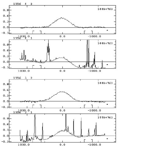
Radio source 1448+762 was observed in continuum at the Effelsberg radio telescope. The receiver output was split on two channels. The signals from one channel were processed by a FPGA processor (Altera Stratix S80) and then sent to the total power detector. The signals from the second channel were applied straight to the total power detector. The bandwidth of the signals applied to the total power detector was equal to 20 MHz. These channels provided two radio telescope outputs: one output with RFI mitigation and another without. Pairs of radio source scans from these outputs were made simultaneously. Because the total power detector was an integral part of the radio telescope backend equipment, the algorithm implemented in FPGA only processed the IF (intermediate frequency) signal with the aim of “cleaning” it of RFI. The analogue input signal was digitized in 12-bit ADC with 40Msamples speed, then processed in FPGA, transformed back into analogue form and applied to the total power detector. Winsorization of the signal in temporal domain ($\gamma=0.05$) was implemented.

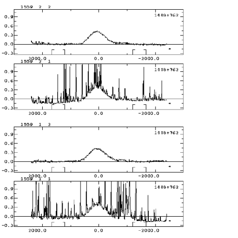
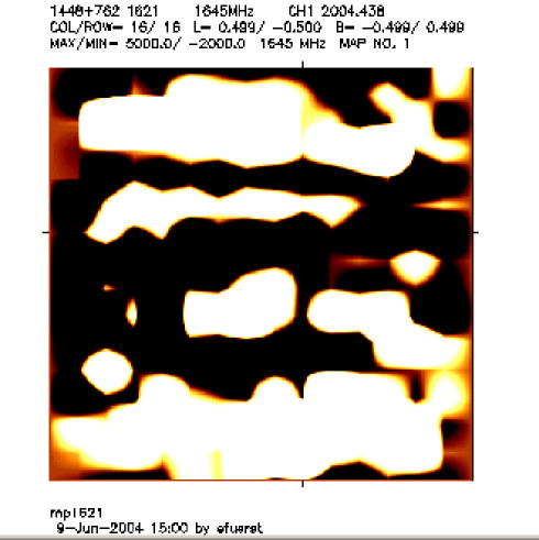
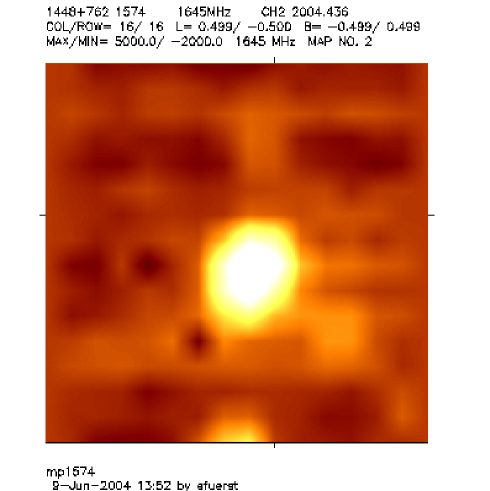
Fig. 8 shows eight scans of the radio source, each scan represented by two panels: the top panel - scan with RFI mitigation, the lower panel - without RFI mitigation. Fig. 9 displays radio images of the source built using scans similar to those in Fig. 8: the left panel - without RFI mitigation, the right panel - with RFI mitigation.

4.2 Pulsar observations at WSRT

A new pulsar machine PUMA-2 has been installed at the Westerbork synthesis radio telescope (WSRT). The radio telescope works in tied-array mode in which all 14 signals from antennas are added in phase , i.e., there is one output (in reality with two polarizations) as for a single dish. The 20 MHz-baseband signals from each of the eight frequency channels of WSRT are digitized (8 bit) and stored in the mass storage system which has sufficient hard disk capacity to support at least 24 hours of continuous observations. Signal processing can therefore be undertaken off-line.

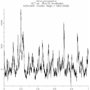
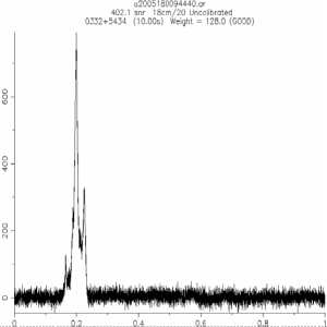
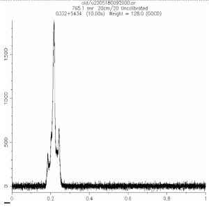
In our experiment a block of data recorded during 10 sec, $40\times 10^{6}$ eight-bit samples/sec, was used. All RFI mitigation processing and the total power detector (TPD) were realized entirely in software during off-line processing. The estimate of variance with exponential weighting was used. Fig. 10 displays the results of processing. Upper row, left panel: TPD outputs for two polarizations calculated from the raw data with RFI, right panel: TPD outputs, RFI removed. Middle row, left panel: example of a time fragment of the power spectrum with RFI; right panel : the same time fragment, RFI removed. Lower row shows pulsar profiles after de-dispersion and folding at the pulsar period, left panel: pulsar profile averaged over 10 sec from both polarizations of raw data, middle panel: similar pulsar profile, RFI removed, right panel: pulsar profile restored with observational data obtained at 1420 MHz without any RFI which is put here for comparison with the profile in the middle panel.

4.3 Radio image synthesis at WSRT

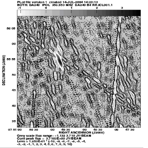
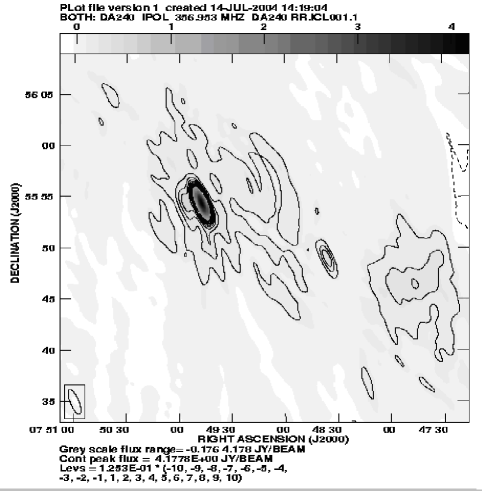
Radio source DA240 was observed at WSRT at a central frequency of 357 MHz with the bandwidth equal to 20 MHz in the presence of strong RFI. The RFI mitigation system (RFIMS) was used for real-time processing (Baan, Fridman & Millenaar, 2004). Analogue baseband signals were digitized (12bit ADC, 40 Msamples/sec), processed in FPGA (Altera StratixS80) and transformed back to analogue form for subsequent processing in the WSRT correlator. The algorithm used for the removal of RFI was similar to the algorithm with exponential weighting, except that the variance was not used as an output, instead “cleaned” , exponentially weighted signals were applied to the correlator.

Radio images of the source DA240 are shown in Fig. 11. Upper row, left panel: image without RFI mitigation; right panel: image with RFI mitigation. Lower row: central parts of the image presented in the same order. The stretched form of the synthesized images is explained by the fact that the observations lasted 8 hours, instead of a full 12 hour aperture synthesis cycle.

RFI mitigation was implemented on each of 14 radio telescopes at WSRT. This may give rise to some distortions because of the difference of equipment characteristics at the different antennas. Other observations were made specifically to judge the “toxicity” of the RFI mitigation procedure. Two pairs of radio images of radio source 4C34.47 were synthesized: one was observed at 1420 MHz with the RFI mitigation system and without it and another at 345 MHz, also with the RFI mitigation system and without it. The first pair of images served as a test for “toxicity” while the second pair demonstrated the effectiveness of RFI mitigation. Both pairwise observational data were stored during simultaneous observations.

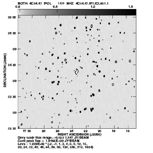
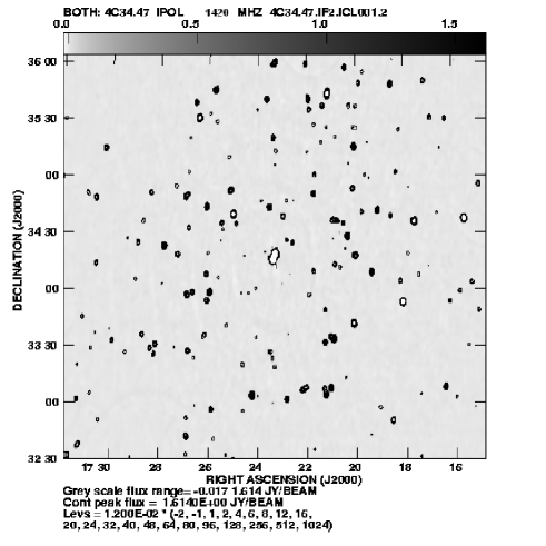
Fig. 12 displays the results of the image synthesis. Upper row, left panel: central frequency 345 MHz, without the RFI mitigation system; right panel: central frequency 345 MHz, with the RFI mitigation system. Notice the difference of intensity levels in the figures. Lower row, left panel: central frequency 1420 MHz without the RFI mitigation system. right panel: central frequency 1420 MHz with the RFI mitigation system. After subtracting one image from the other the rms noise is less than 0.7 mJy/beam which signifies a good similarity in the images.

5 Conclusions

1. Statistical analysis of raw data with the finest available time and frequency resolution can help during observations in an RFI contaminated envinronment. Estimates of variance are an important part of both classical and robust statistics. Growing concern about RFI pollution should persuade the radio astronomy community to pay more attention to a variety of algorithms developed in the realm of robust statistics. Tradional radiometers with simple square-law detectors, spectrum analyzers and correlators must be equipped with these tools. This framework of robust estimates puts the successfully tested blanking of RFI on a more stable foundation.

2. Statistically faithful, robust estimates of variance are especially appropriate for application in an impulse-like strong RFI environment. RFI is effectively suppressed and the accompanying loss in the signal-to-noise ratio is tolerable. Table 3 gives a summary of available RFI mitigation methods which have been proposed during the last years. Some of these have been tested in real observations. Blanking showed truly good results in the case of impulse-like strong RFI. There are slots in the Table 3 where “removing or blanking”” is referred to. The aforementioned robust algorithms can be applied in these particular situations.

3. The results produced from the observations at the Effelsberg radio telescope (image synthesis by beam scanning) and at WSRT (Earth rotation aperture synthesis) included in this article demonstrate the usefulness of this kind of RFI mitigation both in real-time and off-line (pulsars).

4. The choice of a particular algorithm depends on the type and intensity of RFI.The proportion of RFI presence in data is also important. The type of implementation may determine the choice: off-line or real-time. All options are open now. Mass storage systems allow data to be processed off-line on powerful computers. Nowadays both existing radio telesopes future projects (LOFAR, ATA, SKA) will generate such huge amounts of data that real-time processing is vital: DSP, FPGA or supercomputers are possible solutions. Therefore the creation of “ robust” radiometers, spectrum analyzers and correlators is an urgent necessity.

Table 3: The application of RFI mitigation methods

Type of radio	Type of RFI,	Type of RFI,	Observations in continuum	Spectral observations
telescope	intensity	structure
		impulse-like	tolerable	tolerable
	weak	narrow-band	Removing (blanking)	ANC with a reference channel
	RFI		in spectral domain	and post-TPD subtraction;
				HOS analysis
		wideband	ANC with a reference channel	ANC with a reference channel
Single			and post-TPD estimation	and post-TPD estimation
			& subtraction	& subtraction
dish		impulse-like	Removing (blanking)	Removing (blanking)
			in temporal domain	in temporal domain
	strong	narrow-band	Removing (blanking)	ANC with a reference
	RFI		in spectral domain	channel; HOS analysis
		wideband	ANC with	ANC with
			a reference channel	a reference channel
		impulse-like	tolerable	tolerable
	weak	narrow-band	tolerable	Post-correlation ANC with
	RFI			reference channels; HOS analysis
		wideband	tolerable	Post correlation ANC with
Connected				reference channels
radio	strong	impulse-like	Removing (blanking)	Removing (blanking)
interferometer	RFI		in temporal domain	in temporal domain
		narrow-band	Removing (blanking)	ANC with a reference
			in spectral domain	channel. Spatial filtering
		wideband	ANC with a reference	ANC with a reference
			channel. Spatial filtering	channel. Spatial filtering
	weak	impulse-like	tolerable	tolerable
	RFI	narrow-band	tolerable	tolerable
		wideband	tolerable	tolerable
VLBI	strong	impulse-like	Removing (blanking)	Removing (blanking)
	RFI		in temporal domain	in temporal domain
		narrow-band	Removing (blanking)	ANC with a reference
			in spectral domain	channel
		wideband	ANC with a reference	ANC with a reference
			channel	channel

RFI - radio frequency interference.
TPD - total power detector.
ANC - adaptive noise cancellation.
HOS - higher order statistics.

List of captions

Fig. 1. a) The empirical influence function as a function of RFI amplitude, $\sigma=1,n=10^{5}$, the estimates are made with initial data. The curves here and elsewhere are parameterized by the fraction of RFI in the total volume of data: $\epsilon=0.01;0.025;0.5$;
b) estimates made using trimmed data;
c) estimates made using winsorized data;
d) estimates made as the median of pairwise averaged squares;
e) estimates made using the $Qn$ estimate algorithm;
f) estimates made using the biweight variance algorithm;
g) estimates made using the bend midvariance algorithm;
h) estimates made using the algorithm of exponential weighting;
i) estimates made using the algorithm of interquartile range.

Fig. 2. Block diagram of computer simulations: winsorization is used for RFI mitigation when the total power detector is the backend output as in section 4. 1.

Fig. 3. Results of computer simulations with the algorithm shown in Fig. 2:
a) noise with the normal distribution, $\mu=0.0,\sigma=0.5$, no interference;
b) total power detector output, each point in this figure corresponds to squaring and averaging of $10^{4}$ samples in figure a), there are two steps, “up” at point $\#100$ and “down” at point $\#200$ corresponding to the increase of $\sigma$ from value 0.5 to the value $\sigma+\Delta\sigma,\Delta\sigma=0.05$.
c) interference is added to the noise a): random impulses with the Poisson distibution ($\lambda=0.04$) and the lognormal disrtibution of amplitudes (mean=10, standard deviation=5);
d) total power detector output with input signal c);
e) total power detector output with input signal c) and preliminary winsorization (equation (9)), note the difference of scale in d) and e).

Fig. 4. Block diagram of computer simulations: exponential weighting is used for RFI mitigation in the frequency domain when the total power detector is the backend output as in section 4. 2 (pulsar observations)
or the correlator as in section 4. 3. (radiointerferometric observations).

Fig. 5. Results of computer simulations of exponential weighting with the algorithm shown in Fig. 4:
a) time-frequency presentation of power spectrum consisting of system noise, emission and absorption lines and RFI (randomly binary-phase manipulated signals), L=50 time sections of spectrum divided on 256 channels, each spectrum is the mean of $M=100$ instantaneous spectra;
b) power spectrum obtained as a solution to equation (18) for each spectral channel and $M=100$ samples;
c) power spectrum averaged in time, using $L=50$ sample spectra from a);
d) power spectrum averaged in time, using $L=50$ sample spectra from b), i.e., with RFI mitigation.

Fig. 6. Results of computer simulations of exponential weighting with the algorithm shown in Fig. 4:
spectra of interference overlap with spectral lines. Other parameters are similar to Fig. 5,
a) time-frequency presentation of the power spectrum consisting of system noise, emission and absorption lines and RFI; b) power spectrum obtained as a solution to equation (18) for each spectral channel and $M=100$ samples;
c) power spectrum averaged in time, using $L=50$ sample spectra from a);
d) power spectrum averaged in time, using $L=50$ sample spectra from b), i.e., with RFI mitigation. Both spectral lines are clearly visible.

Fig. 7. Results of computer simulations of exponential weighting with the algorithm shown in Fig. 4 when “dirty” and “clean” signals are applied to the correlator; L=50 time sections of the spectrum divided on 256 spectral channels, each spectrum is the mean of $M=100$ instantaneous spectra; the spectra at the first input of the correlator are shown, the spectra at the second input are similar to a) and b):
a) time-frequency presentation of power spectrum consisting of system noise, and RFI (frequency-modulated bursts);
b) power spectrum after RFI mitigation - exponential weighting of each instantaneous spectrum using variances obtained as a solution to equation (18) for each spectral channel and $M=100$ samples;
c) cross-correlation in the presence of RFI and no RFI mitigation, the central 200 channels are shown;
d) cross-correlation in the presence of RFI and with RFI mitigation;
take notice of the difference of the vertical scales in c) and d).

Fig. 8. Examples of RFI mitigation at the Effelsberg radio telescope during observations in continuum at central frequency 1645 MHz, bandwidth 20MHz. A selection of eight scans of the source 1448+762 is represented. Pairwise records were made simultaneously for the channel with RFI mitigation and the channel without RFI mitigation.

Fig. 9. Radio image of the source 1448+762 built using scans similar to those in Fig. 2: left panel - without RFI mitigation, right panel - with RFI mitigation.

Fig. 10. Pulsar B0329+54.07 observed at WSRT at 1625MHz. Data were recorded during 10 sec, 40 Msamples/sec. Upper row, left panel: TPD ouputs for two polarizations, raw data with RFI, right panel: TPD output, RFI removed. Middle row, left panel: time fragment of the running power spectrum with RFI; the same time fragment, RFI removed. Lower row, Left panel: pulsar profile made with raw data over 10 sec, middle panel: pulsar profile, RFI removed, right panel: pulsar profile observed at 1420 MHz, no RFI.

Fig. 11. Radio images of the source DA240 observed at WSRT, central frequency 357 MHz, bandwidth 20 MHz. Upper row, left panel: image without RFI mitigation; right panel: image with RFI mitigation. Lower row: central parts of the images with and without RFI.

Fig. 12 . Radio images of the source 4C34.47 observed at WSRT, bandwidth 20 MHz. Upper row, left panel: central frequency 345 MHz, without RFI mitigation system; right panel: central frequency 345 MHz, with RFI mitigation system. Notice the difference of the intensity levels in the figures. Low row (“toxicity” test), left panel: central frequency 1420 MHz without RFI mitigation system. right panel: central frequency 1420 MHz with RFI mitigation system. After subtracting one image from the other the rms noise is less than 0.7 mJy/beam which signifies a good similarity in the images.

Figure 1: a) The empirical influence function as a function of RFI amplitude, $\sigma=1,n=10^{5}$, estimates made with initial data. The curves here and elsewhere are parameterized by the fraction of RFI in the total volume of data:$\epsilon=0.01;0.025;0.5;$ b) estimates made using trimmed data; c) estimates made using winsorized data; d) estimates made as the median of pairwise averaged squares ; e) estimates made using the $Qn$ estimate algorithm; f) estimates made using the biweight variance algorithm; g) estimates made using the bend midvariance algorithm; h) estimates made using the algorithm of exponential weighting .

i) estimates made using the algorithm of interquartile range.

Figure 2: Block diagram of computer simulations: winsorization is used for RFI mitigation when the total power detector is the backend output as in section 4. 1.

Figure 3: Results of computer simulations with the algorithm shown in Fig. 2: a) noise with the normal distribution, $\mu=0.,\sigma=0.5$, no interference; b) total power detector output, each point in this figure corresponds to squaring and averaging of $10^{4}$ samples in figure a), there are two steps, “up” at point $\#100$ and “down” at point $\#200$ corresponding to the increase of $\sigma$ from value 0.5 to the value $\sigma+\Delta\sigma,\Delta\sigma=0.05$. c) interference is added to the noise a): random impulses with the Poisson distibution ($\lambda=0.004$) and the lognormal disrtibution of amplitudes (mean=12, standard deviation=6); d) total power detector output with input signal c); e) total power detector output with input signal c) and preliminary winsorization, note the difference of scale in d) and e).

Figure 4: Block diagram of computer simulations: exponential weighting is used for RFI mitigation in the frequency domain when the total power detector is the backend output as in section 4. 2 (pulsar observations) or the correlator as in section 4. 3. (radiointerferometric observations).

Figure 5: Results of computer simulations of exponential weighting with the algorithm shown in Fig. 4: a) time-frequency presentation of power spectrum consisting of system noise, emission and absorption lines and RFI (randomly binary-phase manipulated signals), L=50 time sections of spectrum divided on 256 channels, each spectrum is the mean of $M=100$ instantaneous spectra; b) power spectrum obtained as a solution to equation (18) for each spectral channel and $M=100$ samples; c) power spectrum averaged in time, using $L=50$ sample spectra from a); d) power spectrum averaged in time, using $L=50$ sample spectra from b), i.e., with RFI mitigation.

Figure 6: Results of computer simulations of exponential weighting with the algorithm shown in Fig. 4: spectra of interference overlap with spectral lines. Other parameters are similar to Fig. 5, a) time-frequency presentation of the power spectrum consisting of system noise, emission and absorption lines and RFI; b) power spectrum obtained as a solution to equation (18) for each spectral channel and $M=100$ samples; c) power spectrum averaged in time, using $L=50$ sample spectra from a); d) power spectrum averaged in time, using $L=50$ sample spectra from b), i.e., with RFI mitigation. Both spectral lines are clearly visible.

Figure 7: Results of computer simulations of exponential weighting with the algorithm shown in Fig. 4 when “dirty” and “clean” signals are applied to the correlator; L=50 time sections of the spectrum divided on 256 spectral channels, each spectrum is the mean of $M=100$ instantaneous spectra; the spectra at the first input of the correlator are shown, the spectra at the second input are similar to a) and b): a) time-frequency presentation of the power spectrum consisting of system noise, and RFI (frequency-modulated bursts); b) power spectrum after RFI mitigation - exponential weighting of each instantaneous spectrum using variances obtained as a solution to equation (18) for each spectral channel and $M=100$ samples; c) cross-correlation in the presence of RFI and no RFI mitigation, the central 200 channels are shown; d) cross-correlation in the presence of RFI and with RFI mitigation; take notice of the difference of the vertical scales in c) and d).

Figure 8: Examples of RFI mitigation at the Effelsberg radio telescope during observations in continuum at central frequency 1645 MHz, bandwidth 20MHz. A selection of eight scans of the source 1448+762 is represented. The pairwise records were made simultaneously for the channel with RFI mitigation and the channel without RFI mitigation.

Figure 9: Radio image of the source 1448+762 built using scans similar to those in Fig. 2: left panel - without RFI mitigation, right panel - with RFI mitigation.

Figure 10: Pulsar B0329+54.07 observed at WSRT at 1625MHz. Data were recorded during 10 sec, 40 Msamples/sec. Upper row, left panel: TPD ouputs for two polarizations, raw data with RFI, right panel: TPD outputs, RFI removed. Middle row, right panel: time fragment of the running power spectrum with RFI; the same time fragment, RFI removed. Lower row, left panel: pulsar profile made with raw data over 10 sec, middle panel: pulsar profile, RFI removed, right panel: pulsar observed at 1420 MHz, no RFI.

Figure 11: Radio images of the source DA240 observed at WSRT, central frequency 357 MHz, bandwidth 20 MHz, Upper row, left panel: image without RFI mitigation; right panel: image with RFI mitigation. Lower row: central parts of the images with and without RFI.

Figure 12: Radio images of the source 4C34.47 observed at WSRT, bandwidth 20 MHz. Upper row, left panel: central frequency 345 MHz, without RFI mitigation system; right panel: central frequency 345 MHz, with RFI mitigation system. Notice the difference of intensity levels in the figures. Lower row, left panel: central frequency 1420 MHz without RFI mitigation system. right panel: central frequency 1420 MHz with RFI mitigation system. After subtracting one image from the other the rms noise is less than 0.7 mJy/beam which signifies a good similarity in the images.

References

- Baan, Fridman & Millenaar (2004) Baan, W. A., Fridman, P. A. & Millenaar, R. P. 2004, AJ, 128,933
- Barnbaum & Bradley (1998) Barnbaum, C., & Bradley, R. F. 1998, AJ, 116, 2598
- Briggs,Bell & Kesteven (2000) Briggs, F. H., Bell, J. F. & Kesteven, M. J. 2000, AJ, 120, 3351
- David & Nagaraja (2003) David H. A. & Nagaraja, H. N. 2003, Order Statistics, John Wiley & Sons
- Ellingson & Hampson (2003) Ellingson, S. W., & Hampson, G. A. 2003, ApJS147, 167
- Fisher et al. (2005) Fisher, J. R., Qing Zhang, Yibin Zheng, Wilson, S. G. & Bradley. 2005, AJ, 129, 2940
- Fridman & Baan (2001) Fridman, P. A. & Baan, W. 2001, A&A, 378, 327
- Fridman (2001) Fridman, P. A. 2001 A&A, 368, 369
- Jeffs, Li & Warnick (2005) Jeffs, B. D., Li., L. & Warnick, K. 2005, IEEE Trans. Signal Processing, 53, 439
- Hampel (1971) Hampel, F. R. 1971, The Annals of Mathematical Statistics, 42,1887
- Hampel et al. (1986) Hampel, F. R., Ronchetti, E. M., Rousseeuw, P. J. and Stahel, W. A. 1986, Robust Statistics: The Approach Based on Influence Functions, John Wiley & Sons
- Hettmansbperger (1984) Hettmansbperger, T. P. 1984, Statistical Inference Based on Ranks, John Wiley & Sons
- Huber (1964) Huber, P. J. 1964, Ann. Math. Statist. 35, 73.
- Huber (2004) Huber, P. J. 2004, Robust Statistics, John Wiley & Sons
- Kendal & Stuart (1967) Kendal, M. G. & Stuart, A. 1967, The advanced theory of statistics, vol.1, ch. 3
- Kesteven (2007) Kesteven M. 2007, URSI Radio Science Bulletin , 322, 9
- Lax (1985) Lax, D. A. 1985, J. of American Statistical Association, 80, 736
- Mitchell, Robertson & Sault (2005) Mitchell, D. A., Robertson, J. G., & Sault R. J. 2005, AJ, 130, 2424
- Mosteller & Tukey (1977) Mosteller, F. & Tukey, J. M. 1977, Data Analysis and Regression: A Second
- Poulsen, Jeffs & Warnick (2005)
- Rohlfs & Wilson (2003) Rohlfs, K. & Wilson, T. L. 2003, Tools of Radio Astronomy, Springer
- Rousseuw & Croux (1993) Rousseuw, P. J. &Croux, C. 1993, J. of the American Statistical Association, 88, 1273
- Sheskin (2000) Sheskin , D. J. 2000 Handbook of Parametric and Nonparametric Statistical Procedures, Chapman & Hall/CRC, New York
- Shurygin (2000) Shurygin, A. M. 2000, Applied Statistics: Robustness, Estimation and Prediction, Finance& Statistics, Moscow
- Thompson (1982) Thompson, A. R., 1982, IEEE Trans. AP, 30,450
- Thompson (2003) Thompson, A. R., 2003, SKA Memo 34
- Tukey (1960) Tukey, J. W. 1960 , in : Contribution to Probability and Statistics, I. Olkin, Ed., Stanford University Press, Stanford, 448
- van der Waerden (1969) van der Waerden, B. L. 1969, Mathematical Statistics, Springer, Ch. 8
- Wilcox (2004) Wilcox, R. R. 2004, Introduction to Robust Estimation and Hypothesis Testing, Academic Press, Ch.3
- Zhang et al. (2005) Qing Zhang, Yibin Zheng, Wilson, S. G., Fisher, J. R. & Bradley, R. 2005, AJ, 2933