11email: fridman@astron.nl
The self-cohering tied-array
Abstract
Context. Large radio astronomy multi-element interferometers are frequently used as single dishes in a tied-array mode when signals from separate antennas are added. Phase shifts arising during wave propagation through a turbulent atmosphere can significantly reduce the effective area of an equivalent single dish.
Aims. I aim to give estimates of the impact of the ionosphere and troposphere on the effectiveness of a radio interferometer working in tied-array mode.
Methods. Statistical estimates of the effective area are calculated and the power-law of turbulent atmosphere irregularities has been used. A simple method of tied-array calibration using optimization techniques is proposed.
Results. The impact of phase errors on the effectiveness of tied-arrays are given for low and high frequencies. Computer simulations demonstrate the efficacy of the proposed calibration algorithm.
Key Words.:
interferometers – data analysis– statistical1 Introduction
Large radio astronomy multi-element interferometers (VLA, WSRT) are frequently used in the tied-array mode where signals from separate antennas
are added (Thompson et al. 2001, ch. 9.9). The output sum signal can be used in VLBI, pulsar and transients observations (Cordes 2004), SETI signals detection and the direct-to-Earth (DtE) reception of signals from cosmic apparatus (Jones 2004). In all these cases a radio interferometer works as a single-dish antenna
with one output. Partial signals from antennas are properly phased to collect emission from a point-like radio source in the sky and track it during its siderial movement. Standard calibration procedure using a correlator is employed to provide the necessary phase corrections for each individual antenna. Random phase perturbations such as phase shifts arising during wave propagation through the turbulent atmosphere can occur in the course of such observations. These phase errors reduce the total effective area of the tied-array and must be compensated for in real time. Although it is possible to store baseband
data for processing after observations have taken place, the amount of data to be stored places a firm limit to the number of antennas that can be used in this manner.
New large scale projects such as SKA and LOFAR will also be operating in tied-array mode. The impact of ionospheric and tropospheric phase errors on the tied-array is calculated in this paper. A simple method of correcting these errors using the output signal of the tied-array is also proposed here.
2 Tied-array with random phase errors
Voltage produced by the source at the output of the planar tied-array is
| (1) |
where is the source vector, , is the wavelength, is the frequency, - is the signal amplitude at n-th array element, -is the distance between the source and n-th array element, is the number of antennas in the array, is the instrumental phase shift. The distance can be represented as the module of the vector difference , where is the position vector of n-th array element:
| (2) |
are the components of vector and are the components of vector , .
With these new notations (1) can be rewritten as:
| (3) |
An array is directed at when these conditions are satisfied:
| (4) |
The manifold of signals received in other directions () forms the field pattern:
| (5) |
The power pattern is the expected value of the product
| (6) |
where denotes a complex conjugate and denotes a time average.
In the absence of phase errors and in the direction of the radio source, i.e., for . The dc component proportional to the sum of the system noise power at each antenna is omitted here and considered to be a constant value and therefore not relevant.
In the presence of phase errors produced by, for example, the atmosphere, there are additional phase terms in (6) and the power received in the direction is:
| (7) |
where is the variance of the random phase difference for the baseline :
| (8) |
It is assumed that the random phase difference has normal probability distribution with zero mean and variance . In this case (7) was obtained using this relation:
| (9) |
Therefore, the loss produced by the phase errors is equal to:
| (10) |
The variance is the structure phase function of the turbulent atmosphere. The power-law (Kolmogorov) model will be used in the following sections to describe both for the ionosphere and troposphere phase fluctuations (Tatarskii 1978).
2.1 Ionosphere
Phase fluctuations due to the irregular spatial distribution of the refraction index during wave propagation through the ionosphere are described with the power-law model of the turbulence spectrum. The electron density in the ionosphere, considered as a function of spatial coordinates, has variations which are characterized by a structure function of electron density (Thompson et al. 2001, ch. 13):
| (11) |
where , is the constant, is the baseline. This formula can be rewritten for the structure function of the refraction index:
| (12) |
where (electron radius), is the wavelength. Finally, the ionosphere phase structure function is:
| (13) |
where is the total propagation length through the irregularities of the ionosphere, and must be substituted in meters. The value can be estimated from (11) assuming that the ionosphere irregularities of electron density have a maximum dimension equal to :
| (14) |
For example,
for and (day time) we have for ,
for and .
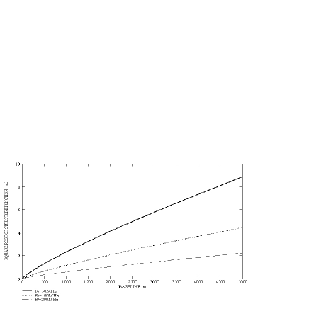
Figure 1a shows the square root of the ionosphere structure function for , and calculated for three frequencies: 50MHz, 100MHz and 200MHz.
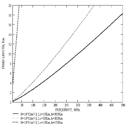
Phase fluctuations can be also characterized by the Fried length:
| (15) |
where is the baseline at which . For the parameters used in Fig. 1a for 50MHz, for 100MHz and
for 200MHz. Fig. 1b shows how Fried length depends on the frequency for the different values of .
The minimal time interval at which it is necessary to repeat calibrations can be calculated from Fried length: where
is the wind velocity. Thus, for example, for and , .
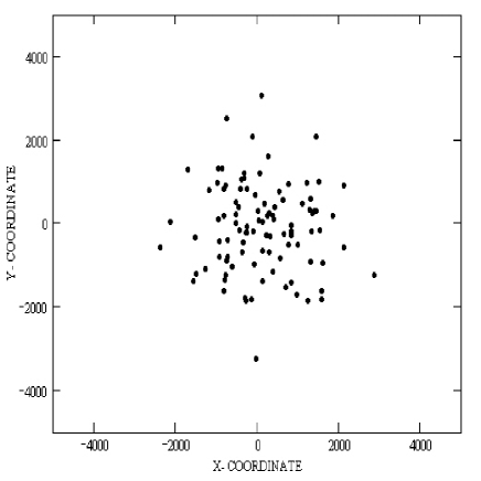
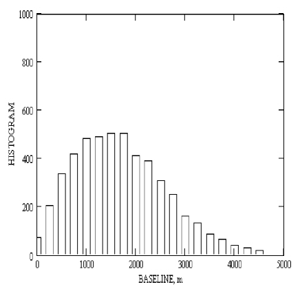
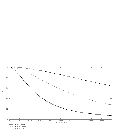
Now the loss produced by ionosphere random phase errors can be calculated in the example of the array whose configuration is shown in Fig. 2a. It is the random planar 100-element array with the coordinates and represented by random normal values with zero mean and standard deviation . For the array shown in Fig. 2a, , therefore the maximum baseline is . The distribution of baselines (histogram) is shown in Fig. 2b . Phase errors are maximal for the largest baselines but their relative number is less than the medium size baselines, therefore the signal loss for the array should take this particular distribution of baselines into account. Fig. 3 demonstrates the dependance of loss versus array size . The curves are calculated for three frequencies: 50, 100 and 200MHz.
2.2 Troposphere
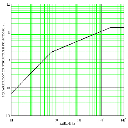
Phase fluctuations due to the irregular spatial distribution of the refraction index during wave propagation through the troposphere are also described in the frame of the power-law spectrum turbulence model. The troposphere phase structure function is (Stotskii 1973, Carilli et al. 1999):
| (16) | |||||
where and are the internal and external scales, respectively, of the isotropic three-dimensional turbulence model,
, and , the latter is determined by global meteorological variations.
Factors and depend on the local content of water vapor and oxygen in the troposphere (weather conditions)
and the values chosen for the purpose of calculation are and .
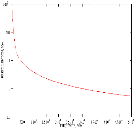
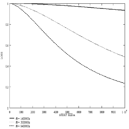
Fig. 4a represents the structure function (16) and Fig. 4b shows the Fried length as a function of the frequency. Fig. 5 demonstrates the dependance of loss
versus array size . The curves are calculated for three frequencies: 1400, 5000 and 8400MHz.
3 Self-cohering
Observations in the tied-array mode (VLBI, transients, DtE) are pre-planned at any time and it is impossible to postpone them in order to choose better atmospheric conditions (for example, night time in the case of the ionosphere). The effectiveness of the synthesized aperture must be maximal during observations which means that periodical calibrations are necessary. Traditional methods of radio interferometer calibration can be applied using the grid of calibration point sources. This calibration must be made in real time with the help of available correlators which must work in parallel with the tied-array adder. Here, another method is proposed which uses the points in the direct images of the field-of-view with calibration sources.
It is presumed that a full calibration with the correlator has already been performed before each tied-array observation. During subsequent observations the total power output of the tied-array is used as a tracking tool and the proposed algorithm will introduce small phase corrections at short time intervals therefore keeping the amplitude of the calibration source at a prescribed level. This has similarities to the approach of (Muller&Buffington 1974) which is also described in (Tyson 1991).
The choice of calibration sources is the same as in traditional methods.
Equation (7) corresponds to the synthesized beam when there are phase errors produced during propagation through the turbulent atmosphere. To eliminate , compensation phase shifts are introduced at each -th array element. The phase of the signal corresponding to the direction at the n-th array element is
| (17) |
where is the compensation phase shift introduced for the correction of - atmospheric phase error. The value of the signal power in the prescribed direction in the image with one or several calibration sources available in the field-of-view (FoV) can be obtained by convolution of the sky intensity with the synthesized beam
| (18) |
where denotes convolution. The similar approach to imaging procedure with an array is considered in the direct imaging scheme, (Wright 2004). Having the output of the total power detector for the direction we can maximize this value by varying , i.e., we have an optimization problem for values of compensation phases. In general, for each direction this problem can be written as
| (19) |
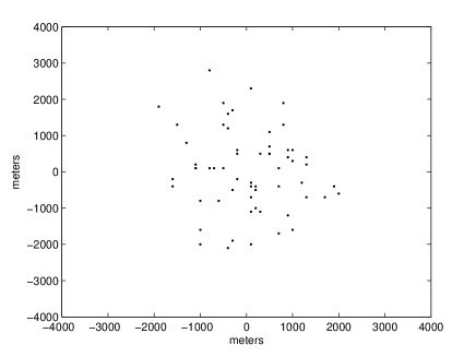
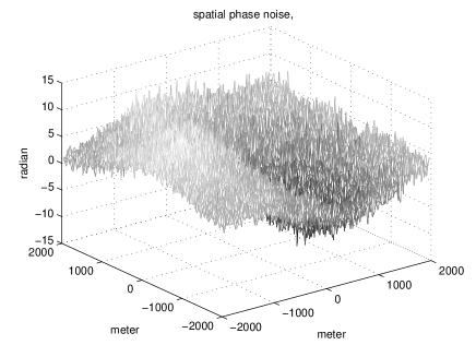
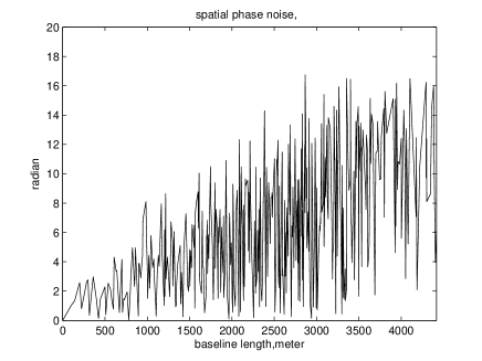
This scheme is illustrated in the following example of computer simulation. The 60-element spatially random planar array is represented in Fig. 6. The phase errors introduced in each of the array element signals are modeled by the two-dimensional random value, Fig. 7, with circular symmetrical spatial spectral density which decreases radially according to the (-11/3) power law. The instantaneous sample of phase errors at frequency 100MHz as a function of baseline length is given in Fig. 8. This high level of phase errors has been chosen to demonstrate the effectiveness of the proposed method.
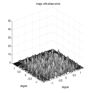
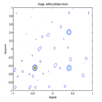
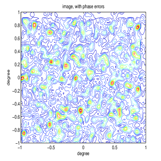
The image containing three point sources is represented in Fig. 9 (left panel) and the synthesized image in the presence of the phase errors (Fig. 8) is shown in Fig. 9 (middle panel).
(isoplanicity being presumed).
The value of the synthesized image in the direction of the largest source (lower left in the image) was used as the cost function. The genetic algorithm(GA) was applied because of the strong multi-modality of the cost function (19) and this algorithm finds the global maximum successfully.
Genetic algorithms search for a solution to a set of variables by the use of simulated evolution, i.e., the survival of the fittest strategy.
In contrast to calculus-based algorithms (conjugate gradients and quasi-Newtonian methods), GA, first introduced in (Holland 1975), exploit a guided random
technique during optimization procedure (Goldberg 1989, Michalewicz 1994, Charbonneau 1995).
GA optimizers are particularly effective when the goal is to find an approximate global maximum in a high-dimension, multi-modal function domain in a near-optimal manner.
They are also largely independent of the starting point or initial guess.
There is parallelism which allows for the exploitation of several areas of the solution space at the same time. This parallelism can be very useful in the implementation of GA on the multi-core platform and FPGA.
In this article, computer simulation has been done on a PC (Intel Pentium, 2.5 Ghz, 1GB RAM) using Matlab 7.6.0. Specific GA operations (selection, crossover and mutation) have taken approximately of the
total computing time: 150 sec for 100 iterations (each iteration is the full cycle of these operations). The rest of the computing time was spent on the calculation of the cost function
(formation of the beam with corrected phases convolution with the image total power output). But these calculations are necessary only in computer simulations:
in reality the values of the cost function are supplied by the tied-array itself (“Nature” does the job).
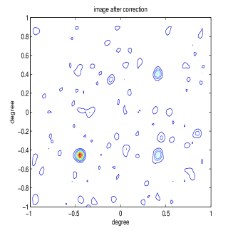
After applying the optimization procedure and introducing the resulting compensation phases the corrected image is shown in Fig. 9 (right panel).
The contour presentations in Fig. 10 correspond to the undistorted image (left panel), the image with phase errors (middle panel) and the image after correction (right panel), respectively.
The corresponding synthesized beam is restored up to 0.94 of its undistorted value.
There are some peculiarities in image processing with non-planar arrays (Perley 1999) but the tied-array mode concerns only point-like sources. Therefore, there is no difference in planar and non-planar arrays in the context of this article (phase irregularities due to atmospheric turbulence), especially for the adaptive calibration procedure described here.
4 Conclusions
-
1.
The effective area of tied arrays may be significantly reduced by ionospheric and tropospheric phase irregularities at low and high frequencies, respectively.
-
2.
Observations are made at times (VLBI, transients monitoring, DtE) when it is impossible to choose quiet atmospheric conditions and real-time calibration is necessary and has to be fulfilled in parallel with observations.
-
3.
The total power at the auxiliary outputs of the tied-array, phased in the direction of calibration sources, can be used on a level with traditional calibration methods using correlators. Multi-beam facilities are necessary for creating these auxiliary outputs. Optimization algorithms (genetic algorithms, simulated annealing) can be used to compensate for propagation phase errors by maximizing the amplitude of a chosen calibration source. The tied array can preserve its correctly phased state during lengthy observations using one or several auxiliary outputs, therefore working in the self-cohering regime. The proposed scheme does not exclude traditional methods of calibration - it is complementary to them.
Acknowledgements.
I am grateful to Roy Smits whose comments were very helpful.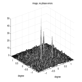

References
- (1) Carilli, C.L., Carlstrom, J.E. & Holdaway, M.A. 1999, in Taylor, G. B., Carilli, C. L., and Perley, R. A., Eds., Synthesis Imaging in Radio Astronomy II (Astronomical Society of the Pacific)
- (2) Charbonneau, P., 1995, APhS, 101, 309
- (3) Cordes, J. M. et al, 2004, New Astronomy Review, 48, 1413 and 1459
- (4) Jones, D. L., 2004, New Astronomy Review, 48, 1543
- (5) Goldberg, D. E. 1989, Genetic Algorithms in Search, Optimization and Machine Learning (Addison-Wesley)
- (6) Holland, J. H. 1975, Adaptation in Natural and Artificial Systems, (University of Michigan Press, Ann Arbor)
- (7) Michalewicz, Z. 1992, Genetic Algorithms + Data structures = Evolution Programs (Springer)
- (8) Muller&Buffington 1974, JOSA, vol.64, 1200
- (9) Perley, R. A., 1999 in Taylor, G. B., Carilli, C. L., and Perley, R. A., Eds., Synthesis Imaging in Radio Astronomy II (Astronomical Society of the Pacific)
- (10) Stotski, A. A. 1973, Radiophys. Quant. Electron, 16, 620
- (11) Tatarskii, V. I. 1978, Wave Propagation in Turbulent Media (John Wiley & Sons, Inc.)
- (12) Thompson, A. R., Moran, J. M. & Swenson, G. W. 2001, Interferometry and Synthesis in Radio Astronomy (John Wiley & Sons, Inc.), ch. 9.9, ch.13
- (13) Tyson, R. K. 1991, Principles of Adaptive Optics (Academic Press, San-Diego)
- (14) Wright, M. 2004, SKA Memo 46