Nonlinear Constants of Quantum Information in Reversible and Irreversible Amplitude Flows

Abstract

We report an approach to quantum open system dynamics that leads to novel nonlinear constant relations governing information flow among the participants. Our treatment is for mixed state systems entangled in a pure state fashion with an unspecified party that was involved in preparing the system for an experimental test, but no longer interacts after $t=0$. Evolution due to subsequent interaction with another party is treated as an amplitude flow channel and uses Schmidt-type bipartite decomposition of the evolving state. We illustrate this with three examples, including both reversible and irreversible information flows, and give formulas for the new nonlinear constraints in each case.

I Introduction

Entanglement, as a term of joint quantum coherence, is one of the most intriguing elements of quantum mechanics and it is crucial in quantum information tasks NC-Preskill . However the existence of an interacting reservoir or environment that leads to decoherence and/or disentanglement Zurek91 ; Chuang-etal95 ; Yu-Eberly04 places an obstacle to the maintenance of joint quantum coherence during any dynamical process maintain coherence . Thus the study and control of entanglement dynamics has received wide attention in recent years (see reviews Mintert-etal05 ; Amico-etal08 ; Yu-EberlySci09 ). There have been studies of entanglement dynamics from many points of view. Examples involve open system treatments Nha-Carmichael04 ; ESD-early ; ESD-later ; ESB ; Kim-etal or closed quantum scenarios such as cavity QED systems Phoenix-Knight ; Bose-etal01 ; Yonac-etal06 ; Yonac-etal07 ; Son-etal02 ; Sainz-Bjork07 ; Yonac-Eberly08 ; Yonac-Eberly10 , spin systems Subrahmanyam04 ; Qian-etal ; Cubitt-etal ; Chan-etal08 ; Wang01 ; Pratt-Eberly01 ; Amico-etal04 ; Yang-etal06 , etc.

Many interesting and sometimes surprising findings such as entanglement sudden death Yu-Eberly04 ; ESD-early ; ESD-later , sudden birth ESB , revivals Kim-etal ; Phoenix-Knight ; Yonac-Eberly08 , dynamical relations with quantum state transfer Subrahmanyam04 ; Qian-etal ; Yang-etal06 , and other exotic types of entanglement evolution have been reported. Such interesting phenomena accompany the idea of tracking entanglement as a carrier of quantum information ESD-later ; ESB ; Kim-etal ; Phoenix-Knight ; Bose-etal01 ; Yonac-etal06 ; Yonac-etal07 ; Son-etal02 ; Sainz-Bjork07 ; Yonac-Eberly08 ; Yonac-Eberly10 ; Subrahmanyam04 ; Qian-etal ; Yang-etal06 ; Cubitt-etal ; Chan-etal08 , a generalization of entanglement swapping swapping .

One consequence has been the discovery of examples of non-trivial “information conservation” among three or more parties Yonac-etal07 ; Sainz-Bjork07 ; Chan-etal08 , arising in cases of sufficiently symmetric interaction Hamiltonians, or special initial states, or reservoirs that are sufficiently small that their state evolution can be followed in detail, such as in perfect-mirror closed-system cavity QED Yonac-etal06 ; Yonac-etal07 ; Sainz-Bjork07 ; Yonac-Eberly08 ; Yonac-Eberly10 and in spin systems Qian-etal ; Yang-etal06 ; Cubitt-etal ; Chan-etal08 . However true reservoirs are complex and difficult to follow, especially if mixed state considerations are important. No general closed-form rules of entanglement transfer are known in such cases.

In this paper we revisit quantum information flow from a different perspective and derive a new class of entanglement constants of motion. Our approach employs amplitude channel dynamics and avoids information loss by tracing, while remaining open to non-Markovian as well as Markovian reservoir behavior. We note that the system of experimental interest, which may be one or more qubits, is almost always prepared in a pure state if possible, and frequently the method of preparation produces a pure entangled state. This means that the system itself is in a mixed rather than a pure state. We assume that the entanglement during state preparation, causing the mixedness, arose via interactions that have ceased prior to the beginning of a period of interest at $t=0$. This period of interest could simply be intended for quantum memory preservation or for specific state manipulations. The static disengaged nature of the prior entanglement partner, and also its lack of specificity in our treatment, reduce it to a vague background object in any further qubit evolution, and for this reason we label it the “Moon”.

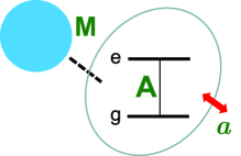
Figure 1: A general sketch of our scenario. The bubble circles the system of interest $A$ and leaves everything else out. The dashed line indicates its entanglement, but not interaction, with the unspecified background “Moon” $M$. The arrow represents interaction between $A$ and an arbitrarily-dimensioned unit $a$, which can be the quantum vacuum reservoir, a single mode cavity, an XY spin chain, etc.

A general sketch of our scenario is given in Fig. 1. Unit $A$ is taken as a two-level system (qubit) and unit $a$ as a separate quantum system of arbitrary dimension interacting with it, nominally a reservoir. The Moon $M$, i.e., the non-interacting, unspecified, and completely static background, is entangled via an earlier preparation stage with $A$.

There obviously remains a wide choice for systems acting as environments that promote evolution of the system of interest after $t=0$. We will illustrate a range of possibilities with concrete results in various specific interaction contexts: spontaneous emission W-W , Jaynes-Cummings (JC) cavity dynamics JC , and XY spin chain interactions Lieb61 . These present very different physical situations and interaction mechanisms, and lead to distinct entanglement dynamics, but they all react similarly to the initial Moon entanglement. Our linked information constants arise from amplitude channel dynamics but do not rely on symmetries of the Hamiltonian or of any special initial state, in contrast to the cases in some previous work Yonac-etal07 ; Chan-etal08 .

II Schmidt analysis of Entanglement

In this section we address our approach to entangled state analysis. The Hamiltonian of our scheme reads

$$H=H_{A}+H_{a}+H_{Aa}+H_{M},$$ (1)

where $H_{A}$, $H_{a}$ and $H_{M}$ are the Hamiltonians of the qubit system $A$, “reservoir” unit $a$ and the previously-interacting Moon $M$ respectively; and $H_{Aa}$ denotes the only existing interaction, that between $A$ and $a$.

We start from the $A$-$M$ entangled preparation state, i.e., the joint superposition state

$$|\psi_{AM}(0)\rangle=\cos\theta|e\rangle|m_{1}\rangle+\sin\theta|g\rangle|m_{2}\rangle,$$ (2)

where $|e\rangle$ and $|g\rangle$ are the excited and ground states of our qubit system $A$, and

$$|m_{1}\rangle=\sum_{l}u_{l}|M_{l}\rangle,\quad\text{and}\quad|m_{2}\rangle=\sum_{l}v_{l}|M_{l}\rangle,$$ (3)

are two normalized Moon states with $\{|M_{l}\rangle\}$ defined as a complete basis set for $M$. It need not be the case generally, but we assume in our example that the Moon states $|m_{1}\rangle$ and $|m_{2}\rangle$ are orthogonal, and because $M$ is not interacting with either $A$ or $a$ they are effectively static:

$$\langle m_{2}(t)|m_{1}(t)\rangle=\langle m_{2}|m_{1}\rangle=0.$$ (4)

We adopt a conventional approach to the interacting partner system labelled $a$, assuming that it is separable from the qubit $A$ at $t=0$, just as in the conventional treatment of a reservoir in quantum open system dynamics Zurek91 ; Chuang-etal95 ; Yu-Eberly04 . Therefore the entire initial state can be written as

$$|\psi_{AaM}(0)\rangle=\Big{(}\cos\theta|e\rangle|m_{1}\rangle+\sin\theta|g\rangle|m_{2}\rangle\Big{)}\otimes|\phi_{1}\rangle,$$ (5)

where $|\phi_{1}\rangle=\sum_{k}i_{k}|k\rangle$ is a normalized state of unit $a$, and $\{|k\rangle\}$ is a complete basis for $a$. Usually $|\phi_{1}\rangle$ is the ground state of part $a$. We note that since $M$ is not interacting, the evolution of the states $|e\rangle|\phi_{1}\rangle$ and $|g\rangle|\phi_{1}\rangle$ are driven only by the Hamiltonian $H_{Aa}$, i.e., the dynamics of the $A$-$a$ part can be separated from $M$. Therefore we will only need to focus on the $A$-$a$ dynamics when we study the time evolution.

Before we proceed to the time dependent state in various specific models in the following sections, we will first discuss the initial Moon entanglement. As we know, the pure-state relation between the two sides of any bi-partition is an $R\times S$ dimensional matrix (where $R$ and $S$ can be any numbers or infinite) that may connote entanglement, but in any event permits a Schmidt-type decomposition of the joint state Grobe-etal ; Ekert ; EberlyLa06 . We use the Schmidt parameter $K$ introduced by Grobe, et al., Grobe-etal as our quantitative measure of entanglement, where $K$ is not simply the dimension of the space NC-Preskill but rather relates to the number of Schmidt modes that make a significant contribution to the state. Therefore we name this parameter $K$ the “Schmidt weight” from now on. The range of this Schmidt weight, $N\geq K\geq 1$ ($N$ is the effective dimension of the space) corresponds to the concurrence range $1\geq\mathcal{C}\geq 0$, when concurrence Wootters98 is also applicable. The upper and lower ends of both ranges denote maximal and zero entanglement, respectively.

The Schmidt weight between two parties $\alpha$ and $\beta$ of a general pure state $|\psi_{\alpha\beta}\rangle$ is defined as

$$K=\Big{[}{\sum_{k}\lambda_{k}^{2}}\Big{]}^{-1},$$ (6)

where these $\lambda_{k}$s are the non-zero eigenvalues of the reduced density matrix for either system, $\rho_{\alpha}$ or $\rho_{\beta}$ EberlyLa06 :

$$\rho_{\beta}=\mathrm{Tr}_{\alpha}[\rho]=\mathrm{Tr}_{\alpha}\Big{[}|\psi_{\alpha\beta}\rangle\langle\psi_{\alpha\beta}|\Big{]}=CC^{{\dagger}}.$$ (7)

Here $C$ is the coefficient matrix connecting the two separate arbitrary complete bases $|n\rangle$ and $|\mu\rangle$ of systems $\alpha$ and $\beta$ respectively, with

$$|\psi_{\alpha\beta}\rangle=\sum_{n,\mu}C(n,\mu)|n_{\alpha}\rangle\otimes|\mu_{\beta}\rangle.$$ (8)

The square roots of $\lambda_{k}$s are also the coefficients of the usual Schmidt decomposition NC-Preskill

$$|\psi_{\alpha\beta}\rangle=\sum_{k}\sqrt{\lambda_{k}}|f_{k}^{\alpha}\rangle\otimes|g_{k}^{\beta}\rangle,$$ (9)

where $|f_{k}^{\alpha}\rangle$ and $|g_{k}^{\beta}\rangle$ are the orthonormal Schmidt states satisfying $\langle f_{k}^{\alpha}|f_{k^{\prime}}^{\alpha}\rangle=\langle g_{k}^{\beta}|g_{k^{\prime}}^{\beta}\rangle=\delta_{kk^{\prime}}$.

Since a general pure state is usually in some arbitrary basis other than the Schmidt basis, it is natural for us to follow the coefficient matrix procedure to calculate the Schmidt weight (6). Accordingly we note from the initial state (5) that the coefficient matrix for the Moon $M$ in the basis of $|m_{1}\rangle$, $|m_{2}\rangle$, $|m_{3}\rangle$, …, and the interacting partner $a$ in the basis $\{|k\rangle\}$, is an $\infty\times\infty$ matrix which is given as

$$C_{M}=\left(\begin{array}[]{cccccccc}i_{1}\cos\theta&..&i_{k}\cos\theta&..&0&...&0&...\\ 0&...&0&...&i_{1}\sin\theta&..&i_{k}\sin\theta&..\\ \vdots&\vdots&\vdots&\vdots&\vdots&\vdots&\vdots&\vdots\end{array}\right),$$ (10)

where the two-dot sign “$..$” represents the elements $i_{k}\cos\theta$ for all the other $k$s, while the three-dot sign “$...$” represents empty rows or columns of zeros for the infinite number of remaining matrix elements. The reduced density matrix however is simply

$$\rho_{M}=C_{M}C_{M}^{{\dagger}}=\left(\begin{array}[]{ccc}\cos^{2}\theta&0&\cdots\\ 0&\sin^{2}\theta&\cdots\\ \vdots&\vdots&\ddots\end{array}\right).$$ (11)

We note that the qubit has reduced the effective interaction space of the Moon to a two dimensional subspace, which means that in this context a two-state subspace of the Moon is in fact quite general. The non-zero eigenvalues of the above matrix are obvious, and the resulting Schmidt weight $K_{M}$ denoting the entanglement between the Moon the remainder is given as

$$K_{M}=\frac{1}{\cos^{4}\theta+\sin^{4}\theta}.$$ (12)

Since the Moon $M$ is not interacting, its internal dynamics only amount to a local unitary transformation Nielsen99 , which will not affect the entanglement between $M$ and the rest, so $K_{M}$ is independent of time. We note that there is no Moon entanglement ($K_{M}=1$) when $\theta=\pi/2$ or 0. In these cases the initial state is a trivial product state. Otherwise $K_{M}>1$. It is particularly interesting when the Moon restricts the $A$-$a$ dynamics and acts as a monitor of the entire entanglement flow. The following sections take a few specific examples of the $A$-$a$ interaction to show the role of Moon entanglement in their particular entanglement information dynamics.

III Spontaneous Emission

In this case the qubit system $A$ is a two level atom and unit $a$ is the quantum vacuum reservoir consisting of the continuum of photon modes. The atom will of course decay to its ground state asymptotically and irreversibly, while one photon is emitted W-W ; Def-gk . We write the Hamiltonian in the usual way as a sum of atom and reservoir contributions:

$$H_{A}=\frac{1}{2}\hbar\omega_{A}\sigma_{A}^{z}\quad\mathrm{and}\quad H_{a}=\sum_{k}\hbar\omega_{k}a_{k}^{{\dagger}}a_{k}.$$ (13)

Here $\sigma_{A}^{z}$ is the usual Pauli matrix, and the usual boson operators represent the reservoir with a continuum of modes, where $a_{k}^{{\dagger}}$ and $a_{k}$ denote the standard creation and annihilation operators respectively, and $\omega_{A}$ and $\omega_{k}$ are the atom and reservoir frequencies. Here $k=1,2,3,...,\infty$, labels the infinitely many modes. The interaction Hamiltonian is also standard:

$$H_{I}=\sum_{k}\hbar(g_{k}^{\ast}\sigma_{A}^{-}a_{k}^{{\dagger}}+g_{k}\sigma_{A}^{+}a_{k}),$$ (14)

where $\sigma_{A}^{+}$, $\sigma_{A}^{-}$ are the usual raising and lowering Pauli operators for the two level system $A$, and the $g_{k}$s are coupling constants between the reservoir and the atom, for which fundamental expressions are well known Def-gk

$$|g_{k}|^{2}=\frac{\omega_{k}}{2\hbar\epsilon_{0}V}{\bf d}_{10}^{2}\cos^{2}\theta.$$ (15)

Here $\theta$ is the angle between the atomic dipole moment $\mathbf{d}_{10}$ and the electric field polarization vector $\hat{\epsilon}_{k}$, and $V$ is the quantization volume. According to our generic description in Eq. (5), the initial state can be rewritten in the spontaneous emission case as

$$|\psi_{AaM}(0)\rangle=\Big{(}\cos\theta|e\rangle|m_{1}\rangle+\sin\theta|g\rangle|m_{2}\rangle\Big{)}\otimes|0\rangle,$$ (16)

where $|e\rangle$ and $|g\rangle$ are the excited and ground state of the two level atom, and we have defined $|\phi_{1}\rangle=|0\rangle$, indicating that all the reservoir modes are in their vacuum states. With the help of the Weisskopf-Wigner treatment W-W ; Def-gk we will find

$$|\psi_{AaM}(t)\rangle = \cos\theta|m_{1}(t)\rangle\Big{(}c_{e}(t)|e\rangle|0\rangle+\sum_{k}c_{k}(t)|g\rangle|1_{k}\rangle\Big{)}$$ (17)

$$+ \sin\theta|m_{2}(t)\rangle|g\rangle|0\rangle,$$

where the coefficient $c_{e}(t)=e^{-\Gamma_{A}t/2}$ with $\Gamma_{A}={\bf d}_{10}^{2}\omega_{A}^{3}/3\pi\epsilon_{0}\hbar c^{3}$ as the natural line width, $|1_{k}\rangle$ denotes that there is one photon in the reservoir mode $k$ while all the rest of the modes are empty and the coefficients

$$c_{k}(t)=g_{k}\frac{1-e^{i(\omega_{A}-\omega_{k})t-\Gamma_{A}t/2}}{\omega_{k}-\omega_{A}+i\Gamma_{A}t/2}$$ (18)

are time dependent. The probability to find the atom in the excited state is $P_{e}(t)=|c_{e}(t)|^{2}=e^{-\Gamma_{A}t}$, which decays to zero asymptotically and irreversibly.

With the dynamical state (17) we can begin to calculate the Schmidt weight $K_{A}(t)$, or $K_{a}(t)$, representing the entanglement between qubit $A$, or vacuum reservoir $a$, and their corresponding remainders. As defined in the last section, the coefficient matrix between $A$ and the remainder for the time dependent state (17) is given as

$$C_{A}=\left(\begin{array}[]{cccccc}c_{e}(t)\cos\theta&0&0&...&0&...\\ 0&\sin\theta&c_{1}(t)\cos\theta&..&c_{k}(t)\cos\theta&..\end{array}\right),$$ (19)

where the two-dot sign “$..$” represents $c_{k}(t)\cos\theta$ for all the other $k$s and the three-dot sign “$...$” again represents empty rows or columns of zeros. Then the reduced density matrix is simply a $2\times 2$ form

$$\rho_{A}=\left(\begin{array}[]{cc}|c_{e}(t)|^{2}\cos^{2}\theta&0\\ 0&\sum_{k}|c_{k}(t)|^{2}\cos^{2}\theta+\sin^{2}\theta\end{array}\right).$$ (20)

Now according to the definition in Eq. (6), we immediately have the qubit entanglement $K_{A}(t)$ given by the expression

$$K_{A}(t)=\frac{2}{[2\cos^{2}\theta e^{-\Gamma_{A}t}-1]^{2}+1}.$$ (21)

We note that at $t=0$,

$$K_{A}(0)=\frac{1}{\cos^{4}\theta+\sin^{4}\theta},$$ (22)

a finite number that is naturally the same as the constant Moon entanglement (12). As time goes on, the probability of the atom in the excited state $P_{e}(t)$ decays gradually, and at $t=\infty$ the probability is completely transferred to the ground state and leaves the atom in a product state with its remainder system, which means eventually $A$ is disentangled from the rest of the universe, and the Schmidt weight $K_{A}(\infty)=1$. Fig. 2 illustrates the behavior $K_{A}(t)$ as a function of $t$ at four different $\theta$ values. We note that in the region when $\sin^{2}\theta<\cos^{2}\theta$, $K_{A}(t)$ starts from a finite value, evolves to a local maximum and then decays irreversibly to $1$ as is shown in Fig. 2 (a) and (b). However when $\sin^{2}\theta\geq\cos^{2}\theta$ as is shown in Fig. 2 (c) and (d), $K_{A}(t)$ decays directly and irreversibly to $1$.

Now let us focus on the reservoir entanglement. From the time dependent state (17) we see that the coefficient matrix of reservoir $a$ is given as

$$C_{a}=\left(\begin{array}[]{cccc}0&\sin\theta&c_{e}(t)\cos\theta&...\\ c_{1}(t)\cos\theta&0&0&...\\ ..&\vdots&\vdots&\vdots\\ c_{k}(t)\cos\theta&\vdots&\vdots&\vdots\\ ..&\vdots&\vdots&\vdots\end{array}\right).$$ (23)

Then the reduced density matrix is given by $\rho_{a}=C_{a}C_{a}^{{\dagger}}$ with an infinite number of non-zero eigenvalues

$${\lambda_{0}} {=} |c_{e}(t)|^{2}\cos^{2}\theta+\sin^{2}\theta,$$ (24)

$${\lambda_{k}} {=} |c_{k}(t)|^{2}\cos^{2}\theta,$$ (25)

for $k=1,2,3,...,\infty$. Now from the definition (6) we find the reservoir Schmidt weight:

$$K_{a}(t)=\frac{2}{[2\cos^{2}\theta(1-e^{-\Gamma_{A}t})-1]^{2}+1}.$$ (26)

Obviously the reservoir is initially not entangled. Then its entanglement gradually increases, and at time $t=(\ln 2)/\Gamma_{A}$ we find $K_{A}(t)=K_{a}(t)$. When time goes to infinity we note

$$K_{a}(\infty)=K_{A}(0)=\frac{1}{\cos^{4}\theta+\sin^{4}\theta}.$$ (27)

That is, the final reservoir entanglement $K_{a}(\infty)$ equals the initial qubit entanglement $K_{A}(0)$. Fig. 2 plots the behavior of $K_{a}(t)$ as a function of $t$ for various $\theta$ values. We note that in the region when $\sin^{2}\theta<\cos^{2}\theta$ as is shown in Fig. 2 (a) and (b), $K_{a}(t)$ starts from zero entanglement, reaches a maximum and then evolves to a finite value $K_{A}(0)$ in the end. In the opposite region of $\theta$ as shown in Fig. 2 (c) and (d), it increases directly and irreversibly to the value $K_{A}(0)$.

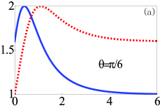
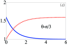
Figure 2: Time dependence of Schmidt weights $K_{A}(t)$ and $K_{a}(t)$ for the spontaneous emission dynamics at different values of $\theta$. In each of the four plots, the blue solid and the red dotted lines denote $K_{A}(t)$ and $K_{a}(t)$ respectively, and the x axis represents time $t$ with unit $1/\Gamma_{A}$. Complementary behavior of the two Schmidt weights is shown clearly in plots (c) and (d) where $\sin^{2}\theta\geq\cos^{2}\theta$.

To summarize, the qubit entanglement $K_{A}(t)$ starts at a finite value and decays completely to zero entanglement, while $K_{a}(t)$ starts from no entanglement and eventually inherits the exact amount of the qubit’s initial entanglement $K_{A}(0)$. This is exactly equal to the Moon entanglement $K_{M}$, so one can see that the unknown Moon’s entanglement (12) has jumped into the picture. It is constant itself, but it acts as a kind of buffer to restrict information flow to and from $A$. In another way of speaking, we could say that there is only a certain amount of “free” entanglement able to be exchanged, which is determined by the Moon.

To take a further step and without loss of generality, we now assume $\sin^{2}\theta\geq\cos^{2}\theta$ for convenience. Then we find two equalities connecting each of $K_{A}(t)$ and $K_{a}(t)$ to $K_{M}$:

$$\sqrt{\frac{2}{K_{A}(t)}-1}-\sqrt{\frac{2}{K_{M}}-1}=2(1-e^{-\Gamma_{A}t})\cos^{2}\theta,$$ (28)

$$\sqrt{\frac{2}{K_{a}(t)}-1}-\sqrt{\frac{2}{K_{M}}-1}=2e^{-\Gamma_{A}t}\cos^{2}\theta.$$ (29)

We note that both $K_{A}(t)$ and $K_{a}(t)$ are controlled by the Moon in a non-linear way. This control leads to a novel conservation relation between $A$ and $a$ in a pairwise fashion:

$$\sqrt{\frac{2}{K_{A}(t)}-1}+\sqrt{\frac{2}{K_{a}(t)}-1}=1+\sqrt{\frac{2}{K_{M}}-1}.$$ (30)

Although $K_{A}(t)$ and $K_{a}(t)$ are time dependent quantities they combine in this way to a constant determined only by the Moon entanglement $K_{M}$.

Because of the restriction of the Moon entanglement we note from the conservation relation (30) that in this region $\sin^{2}\theta\geq\cos^{2}\theta$ or $\theta\in[\pi/4,3\pi/4]$, the decreasing of $K_{A}(t)$ is accompanied by the increasing of $K_{a}(t)$ as is shown in Fig. 2 (c) and (d). To see quantitatively this complementary relation let us take $\theta=\pi/4$ as an example. Then the time dependent qubit and reservoir Schmidt weights simplify to

$$K_{A}(t) = \frac{2}{(1-e^{-\Gamma_{A}t})^{2}+1},$$ (31)

$$K_{a}(t) = \frac{2}{e^{-2\Gamma_{A}t}+1}.$$ (32)

Obviously these two equations for $K_{A}(t)$ and $K_{a}(t)$ depend on time in an opposite way. It is interesting to note that the parameter $\Gamma_{A}$, which represents a collective coupling between the atom and the reservoir modes, is also controlling the two entanglements inversely. This is because of the Moon entanglement $K_{M}$, which acts as a buffer to both entanglements $K_{A}(t)$ and $K_{a}(t)$ but substantially in a opposite way through $\Gamma_{A}$ (see Eqs. (28) and (29)).

We remark that for $\sin^{2}\theta<\cos^{2}\theta$, a similar relation to Eq. (30) can be achieved with only a modification of signs. In this case $K_{A}(t)$ and $K_{a}(t)$ are not always complementary any more as Fig. 2 (a) and (b) show for wide regions of $t$. However $K_{A}(t)$ and $K_{a}(t)$ still stand in a time-invariant relation similar to (30) and are connected only by $K_{M}$.

IV Jaynes-Cummings interaction

Spontaneous emission is an example of an irreversible process. In this section we will turn to a simple example when the $A$-$a$ interaction is reversible, following the JC model JC . Thus qubit $A$ is still a two level atom while unit $a$ is now simply a single mode lossless cavity. Local entanglement dynamics between the atom and the field in the JC model was first studied by Phoenix and Knight Phoenix-Knight by expressing the entangled atom-field state in terms of the eigenstates and eigenvalues of both the field and atomic operators, and revival physics Eberly-etal80 ; Eberly-etal81 ; Yoo85 played a key role in the dynamics. Later, it was shown by Son, et al., Son-etal02 that entanglement between two non-interacting qubits can be generated through the qubits’ local interactions with their corresponding JC cavities that are initially in an entangled two-mode squeezed state. Lee, et al., Kim-etal showed that there is actually entanglement reciprocation between the two qubits and their corresponding continuous-variable systems such as JC cavities. Recently, the JC model was revisited by Yönaç, et al., Yonac-etal06 ; Yonac-etal07 ; Yonac-Eberly08 , and by Sainz and Björk Sainz-Bjork07 , to illustrate the entanglement sudden death phenomenon Yu-Eberly04 , as well as to track the entanglement flow, and conservation relations were found by both groups Yonac-etal07 ; Sainz-Bjork07 .

Here we will continue to track the entanglement information in the JC dynamics, but in addition will account quantitatively for the role of the non-interacting unknown Moon. The JC Hamiltonian is given as

$$H_{Aa}=\frac{1}{2}\hbar\omega_{A}\sigma_{A}^{z}+\hbar g(a^{{\dagger}}\sigma_{A}^{-}+a\sigma_{A}^{+})+\hbar\omega_{a}a^{{\dagger}}a,$$ (33)

where $\sigma_{A}^{z}$, $\sigma_{A}^{\pm}$ are the usual Pauli matrices describing the two level atom $A$, while $a^{{\dagger}}$ and $a$ denote the standard creation and annihilation operators for the single mode cavity. The atom and cavity frequencies are $\omega_{A}$ and $\omega_{a}$, respectively, and $g$ is the coupling constant between the atom and the cavity. For convenience we take the resonant condition when $\omega_{A}=\omega_{a}$.

Now from the generic expression (5) the initial state for the JC model can be written as

$$|\psi_{AaM}(0)\rangle=\Big{(}\cos\theta|e\rangle|m_{1}\rangle+\sin\theta|g\rangle|m_{2}\rangle\Big{)}\otimes|0\rangle,$$ (34)

where $|e\rangle$ and $|g\rangle$ are the excited and ground state of the two level atom, and we have defined $|\phi_{1}\rangle=|0\rangle$ as the zero photon state of the cavity. From the Jaynes-Cummings treatment JC we will have the time dependent state as

$$|\psi_{AaM}(t)\rangle = \cos\theta|m_{1}(t)\rangle\Big{(}e^{i\omega_{A}t/2\hbar}\cos gt|e\rangle|0\rangle$$ (35)

$$- ie^{-i\omega_{A}t/2\hbar}\sin gt|g\rangle|1\rangle\Big{)}$$

$$+ \sin\theta|m_{2}(t)\rangle|g\rangle|0\rangle,$$

where $|1\rangle$ means that there is one photon in the cavity. If we follow the same Schmidt calculations as in the last section, we will have entanglement $K_{A}(t)$ between atom $A$ and the rest of the universe as

$$K_{A}(t)=\frac{2}{[2\cos^{2}\theta\cos^{2}gt-1]^{2}+1}.$$ (36)

That is, we find expression (21) again, except that $e^{-\Gamma_{A}t}$ has been replaced by $\cos^{2}gt$. This is just the replacement of one formula for excited state probability by another, as the nature of the amplitude decay channel requires.

While the initial qubit entanglement $K_{A}(0)$ again has a value equal to the Moon entanglement (12), in the JC dynamics $K_{A}(t)$ has a period of $\tau=\pi/g$ instead of decaying irreversibly as in the spontaneous emission case. We see at the half period time the atom loses all of its entanglement: $K_{A}(t=\tau/2)=1$. Then it evolves to the initial value $K_{A}(0)$ at $t=\tau$. Fig. 3 shows this periodic behavior of $K_{A}(t)$ plotted as a function of $t$ at different $\theta$ values. Recovery of atom-field and atom-atom entanglement in the JC dynamics was already shown previously in Refs. Phoenix-Knight ; Bose-etal01 ; Yonac-etal06 ; Yonac-etal07 ; Son-etal02 ; Sainz-Bjork07 ; Yonac-Eberly08 . However, here our result shows a different type of entanglement recovery, because $K_{A}(t)$ denotes another type of entanglement, this time including the unspecified non-interacting Moon as well as the cavity.

The cavity entanglement $K_{a}(t)$,

$$K_{a}(t)=\frac{2}{[2\cos^{2}\theta\sin^{2}gt-1]^{2}+1},$$ (37)

is also predictable if we look to (26) and see that $1-e^{-\Gamma_{A}t}$ should be converted to $\sin^{2}gt$ because both are expressions for the ground state probability. We note that $K_{a}(t)$ is also periodic. It is initially not entangled with its remainder ($K_{a}(0)=1$), and then increases with time. At $t=\pi/4g$, we have $K_{a}(t)=K_{A}(t)$, and at the half period time we see that

$$K_{a}(t=\tau/2)=K_{A}(0)=K_{M},$$ (38)

exactly the same as $K_{A}(0)$ entanglement. Again Fig. 3 illustrates the periodic behavior of $K_{a}(t)$ as a function of $t$ at various $\theta$ values. When compared with the behavior of the qubit entanglement we see that the amount of entanglement $K_{M}$ has been completely transferred from $K_{A}(t)$ to $K_{a}(t)$ at the half period time $t=\tau/2$. After this, however, the entanglement is repeatedly transferred back and forth between $K_{A}(t)$ and $K_{a}(t)$. This is the major difference from the spontaneous emission case where the reversible process is absent.

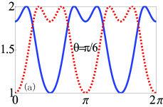
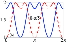
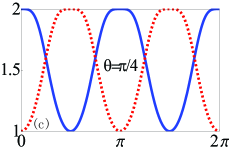
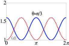
Figure 3: Time dependence of Schmidt weights $K_{A}(t)$ and $K_{a}(t)$ for the JC dynamics at different values of $\theta$. In each of the four plots, the blue solid and the red dotted lines denote $K_{A}(t)$ and $K_{a}(t)$ respectively, and the x axis represents time $t$ with unit $1/g$. Complementary behavior of the two Schmidt weights is shown clearly in plots (c) and (d) where $\sin^{2}\theta\geq\cos^{2}\theta$.

Again we work in the sector when $\sin^{2}\theta\geq\cos^{2}\theta$ for convenience and see that both of the entanglements $K_{A}(t)$ and $K_{a}(t)$ are restricted by the constant Moon entanglement $K_{M}$ in the following non-linear time-dependent way:

$$\sqrt{\frac{2}{K_{A}(t)}-1}-\sqrt{\frac{2}{K_{M}}-1} = 2\sin^{2}gt\cos^{2}\theta,$$ (39)

$$\sqrt{\frac{2}{K_{a}(t)}-1}-\sqrt{\frac{2}{K_{M}}-1} = 2\cos^{2}gt\cos^{2}\theta.$$ (40)

This periodic time dependent control of the two Schmidt weights by the Moon entanglement is different from the spontaneous emission case. However, the two equalities also lead to the same generic entanglement conservation relation

$$\sqrt{\frac{2}{K_{A}(t)}-1}+\sqrt{\frac{2}{K_{a}(t)}-1}=1+\sqrt{\frac{2}{K_{M}}-1}.$$ (41)

Therefore in the JC model case the time dependent Schmidt weights $K_{A}(t)$ and $K_{a}(t)$ are also restricted by the constant Moon entanglement $K_{M}$. We see clearly here that the decrease of $K_{A}(t)$ is accompanied by the increase of $K_{a}(t)$ and vice versa as is shown in Fig. 3 (c) and (d). To show quantitatively we again take $\theta=\pi/4$ as in Fig. 3 (c) to follow this complementary relation of the two entanglements:

$$K_{A}(t) = \frac{2}{\sin^{4}gt+1},$$ (42)

$$K_{a}(t) = \frac{2}{\cos^{4}gt+1},$$ (43)

which are the exact analogs of (31) and (32).

V XY Spin Interaction

We now move to a condensed matter context and take a final example when the $A$-$a$ connection is a Heisenberg exchange interaction or spin-spin interaction. Here qubit system $A$ is a spin one-half particle while unit $a$ is now an $N$-spin XY chain Lieb61 (see Fig. 4), a simplified model for strongly correlated materials such as ferromagnets, antiferromagnets, etc.

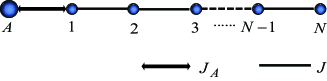
Figure 4: Scheme of qubit $A$ interacting with an XY chain. The big blue dot represents the qubit $A$ while the $N$ small dots represent the spins in the XY chain. The arrow indicates interaction between $A$ and the first spin in the chain with coupling constant $J_{A}$ while the solid segments connect the nearest neighbor sites in the chain with coupling constant $J$.

The first studies of entanglement flow in spin chains focused on few-qubit chains ($N\leq 6$) and the $W$ state Wang01 , and also entanglement dispersion in long chains ($N\gg 1$) Pratt-Eberly01 . Amico, et al. Amico-etal04 studied the propagation of a pairwise entangled state through an XY spin chain, and found that singlet-like states are transmitted with higher fidelity than other maximally entangled states. Here we also focus on the entanglement dynamics, not to transport the entanglement, but to track the information flow by taking into account the role of the entangled Moon. The interaction Hamiltonian of our scheme is given as

$$H_{Aa} = J_{A}(\sigma_{A}^{+}\sigma_{1}^{-}+\sigma_{A}^{-}\sigma_{1}^{+})$$ (44)

$$+ \sum_{n=1}^{N-1}J(\sigma_{n}^{+}\sigma_{n+1}^{-}+\sigma_{n}^{-}\sigma_{n+1}^{+}),$$

where $\sigma^{\pm}$ are the usual Pauli matrices describing the spins, $J_{A}$ is the coupling constant between spin $A$ and the first spin $\sigma_{1}$ of the XY chain, and $J$ is the coupling constant between the nearest neighbor sites inside the XY chain. Now we take $J_{A}=J$ for convenience. This model can be transformed through a Jordan-Wigner transformation Jordan28 into a set of free fermions (see for example Ref. Qian-Song06 ) and thus can be solved exactly Lieb61 . From the perspective of the Jordan-Wigner transformation, the XY model is equivalent here to a free fermion hopping model or Tight-Binding model describing phonon systems.

For the XY Hamiltonian $H_{Aa}$ the exact $N+1$ eigenstates are given as

$$|k\rangle = \sqrt{\frac{2}{N+2}}\sin\left(\frac{k\pi}{N+2}\right)\left|\uparrow\right\rangle|0\rangle$$ (45)

$$+ \sqrt{\frac{2}{N+2}}\sum_{n=1}^{N}\sin\left[\frac{\left(n+1\right)k\pi}{N+2}\right]\left|\downarrow\right\rangle|1_{n}\rangle,$$

where $\left|\uparrow\right\rangle$ and $\left|\downarrow\right\rangle$ are the spin up and down states for our qubit $A$, and $|1_{n}\rangle$, $|0\rangle$ are the states of the XY spin chain with $|1_{n}\rangle$ indicating there is a spin up at the $n$th site while all the rest are in the spin down state and $|0\rangle$ meaning all the sites from site $1$ to site $N$ are in the down state. Here $k=1,2,3,...,N+1$ represent the $N+1$ eigenstates. The corresponding eigenvalues are

$$E_{k}=2J\cos\left(\frac{k\pi}{N+2}\right).$$ (46)

Then the evolution operator can be written as

$$U_{Aa}(t)=\sum_{k=1}^{N+1}e^{-iE_{k}t}|k\rangle\langle k|.$$ (47)

Again from the generic initial state (5) we have here for the XY model

$$|\psi_{AaM}(0)\rangle=\Big{(}\cos\theta\left|\uparrow\right\rangle|m_{1}\rangle+\sin\theta\left|\downarrow\right\rangle|m_{2}\rangle\Big{)}\otimes|0\rangle,$$ (48)

where we have defined $|\phi_{1}\rangle=|0\rangle$ to represent all the $N$ spins in the XY chain that are in the down state. Then the time dependent state can be achieved as

$$|\psi_{AaM}(t)\rangle = \cos\theta|m_{1}(t)\rangle\Big{(}c_{e}(t)|\uparrow\rangle|0\rangle+\sum_{n=1}^{N}c_{n}(t)\left|\downarrow\right\rangle|1_{n}\rangle\Big{)}$$ (49)

$$+ \sin\theta|m_{2}(t)\rangle|\downarrow\rangle|0\rangle.$$

where we have defined

$$c_{e}(t)=\sum_{k=1}^{N+1}\frac{2e^{-iE_{k}t}}{N+2}\sin\left(\frac{k\pi}{N+2}\right)\sin\left(\frac{k\pi}{N+2}\right),$$ (50)

$$c_{n}(t)=\sum_{k=1}^{N+1}\frac{2e^{-iE_{k}t}}{N+2}\sin\left(\frac{k\pi}{N+2}\right)\sin\left(\frac{n+1}{N+2}k\pi\right).$$ (51)

Since $c_{e}(t)$ and $c_{n}(t)$ are complicated expressions for arbitrary number $N$, here we take $N=10$ as an example to illustrate their properties. Then we have

$$c_{e}(t) = \frac{1}{12}\Big{[}2+3\cos(Jt)+2\cos(\sqrt{2}Jt)+\cos(\sqrt{3}Jt)$$ (52)

$$+ (2+\sqrt{3})\cos\frac{(\sqrt{3}-1)Jt}{\sqrt{2}}$$

$$+ (2-\sqrt{3})\cos\frac{(\sqrt{3}+1)Jt}{\sqrt{2}}\Big{]}.$$

We note that the five cosine functions have five different periods and the ratio of any two periods is irrational. Therefore the five quantities will not have a common period, which means that $c_{e}(t)$ will oscillate all the time but without a fixed period. Now we define $f(J,t)=|c_{e}(t)|^{2}$ and note that it can vary from $0$ to $1$. There are infinitely many solutions for $f(J,t)=0$ as a function of time $t$, say $t=\tau_{i}$, with $i=1,2,3,...,\infty$.

If we follow the same Schmidt calculations as in the last two sections we will find the Schmidt weight $K_{A}(t)$ between the qubit spin $A$ and the remainder as

$$K_{A}(t)=\frac{2}{[2f(J,t)\cos^{2}\theta-1]^{2}+1}.$$ (53)

We note that the qubit entanglement $K_{A}(t)$ is also oscillating as determined by $f(J,t)$. As the amplitude channel requires, it starts at the familiar same value $K_{A}(0)=K_{M}$, and in this example evolves to zero entanglement at the time points $\tau_{i}$. After each of these zeros, $K_{A}(t)$ will increase to a local maximum point and then decay to $1$ again at the next time point $\tau_{i+1}$. Fig. 5 illustrates this particular behavior of $K_{A}(t)$ as a function of $t$ at different values of $\theta$. Such aperiodic behavior is intermediate to the previous two examples showing irreversible decay and periodic oscillation, and is expected on the basis of the irrationally related spin-chain eigenfrequencies.

Now we come to the XY chain entanglement $K_{a}(t)$ representing the entanglement between the chain and its remainder, i.e., the end spin $A$ and the Moon $M$. It is related to $K_{A}$ in the usual way. We just replace $f(J,t)$ by $1-f(J,t)$ and obtain:

$$K_{a}(t)=\frac{2}{[2\cos^{2}\theta(1-f(J,t))-1]^{2}+1}.$$ (54)

So the chain entanglement also oscillates with $f(J,t)$. In general, the entanglement will be transferred back and forth between $K_{A}(t)$ and $K_{a}(t)$ with $K_{M}$ the upper limit of entanglement that can be transferred just as the previous two cases.

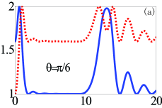
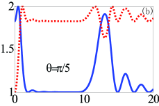
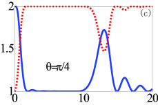
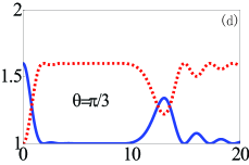
Figure 5: Time dependence of Schmidt weights $K_{A}(t)$ and $K_{a}(t)$ for the XY spin chain dynamics at different values of $\theta$. In each of the four plots, the solid and the dotted lines denote $K_{A}(t)$ and $K_{a}(t)$ respectively, and the x axis represents time $t$ with unit $1/J$. Complementary behavior of the two Schmidt weights is shown clearly in plots (c) and (d) where $\sin^{2}\theta\geq\cos^{2}\theta$.

As expected, restrictions on entanglement flow follow the previous examples. In the regime $\sin^{2}\theta\geq\cos^{2}\theta$ we can simply repeat relations (39) and (40) by replacing $\cos^{2}gt$ with $f(J,t)$:

$$\sqrt{\frac{2}{K_{A}(t)}-1}-\sqrt{\frac{2}{K_{M}}-1}=2\left[1-f(J,t)\right]\cos^{2}\theta,$$ (55)

$$\sqrt{\frac{2}{K_{a}(t)}-1}-\sqrt{\frac{2}{K_{M}}-1}=2f(J,t)\cos^{2}\theta,.$$ (56)

Naturally, the same non-linear conservation relation (41) is recovered, and again the $A$ and $a$ entanglements behave complementarily, this time as a function of $Jt$ as shown in Fig. 5 (c) and (d).

VI Summary

In summary we have studied entanglement information flow from the perspective of a dynamical qubit $A$ in an initially mixed state, a state that was generated by an entanglement associated with a prior process, which we can loosely assign to an experimental preparation stage. Using Schmidt-decomposition rather than master-equation analysis, we derived conservation statements for the separate degrees of quantum entanglement of the qubit and of its interacting reservoir, and showed their relation to the entanglement of the unspecified background party we called the Moon, which was initially entangled but at $t=0$ ceased to interact with either the qubit $A$ or its environment $a$.

The new forms of entanglement conservation relations are nonlinear connections between quantum memories, dependent on the restrictions implied by amplitude flow channel dynamics. One can say that the channel’s enforcement of excitation number conservation in the qubit-reservoir interaction is the root cause of the entanglement and its flow. This is closely analogous to the continuous entanglement between transverse momenta in spontaneous parametric down conversion, which arises from the enforcement of simultaneous momentum and energy conservation on the two-photon amplitude in the creation of the signal and idler photons.

Although unspecified, and ignored in previous open system analyses, the Moon can be assigned responsibility for the initial impurity of the qubit state. The three-part total universe ($A$ + $a$ + $M$) was bi-partitioned three ways in order to evaluate the respective Schmidt weights, as indicators of entanglements in three specific interaction models (spontaneous emission, JC interaction, and XY spin chain). These were analyzed to illustrate the flow of quantum information in different contexts, including both discrete and continuous versions of the reservoir system labelled $a$. Although the influences on individual entanglements differ in various ways, the amplitude flow common to them produces entanglement conservation relations in the same form. One can say that the non-specified Moon retains a kind of influence on the system of interest whether we are “looking” (through interaction) at it or not. The qubit can feel, through the entanglement conservation relation but not through interaction, that the Moon is there.

There can be interesting consequences when the Moon also has a significant dynamical evolution, although still not interacting with $A$, because its entanglement with $A$ can then be assigned to part rather than all of it. This discussion will be undertaken elsewhere Qian-Eberly10 . Finally we would like to comment on the inverse dependence of $K_{A}(t)$ and $K_{a}(t)$ on the interaction parameters as discussed at the end of our three examples. It will be particularly interesting if, for some systems, the interaction constant can be adjustable (e.g., the coupling constant of a spin-spin interaction). Especially in the thermodynamic limit interesting phenomena such as quantum phase transitions Sachdev ; Osterloh-etal02 may arise from changes of the interaction parameter. The behavior of the entanglements in the vicinity of the critical point will be extremely interesting (see for example Qian-etal05 and references therein).

We acknowledge helpful conversations with Profs. L. Davidovich and Ting Yu, and partial financial support from the following: DARPA HR0011-09-1-0008, ARO W911NF-09-1-0385, NSF PHY-0855701.

References

- (1) M. A. Nielsen and I. L. Chuang, Quantum Computation and Quantum Information (Cambridge Univ. Press, 2000); and J. Preskill, Quantum Information and Computation, Caltech Lecture Notes for Ph219/CS219.
- (2) W.H. Zurek, Phys. Today 44, 36 (1991); W.H. Zurek, Rev. Mod. Phys. 75, 715 (2003).
- (3) I.L. Chuang, R. Laflamme, P.W. Shor, and W.H. Zurek, Science 270, 1633 (1995).
- (4) T. Yu and J.H. Eberly, Phys. Rev. Lett. 93, 140404 (2004).
- (5) W.G. Unruh, Phys. Rev. A 51, 992 (1995); D.P. DiVincenzo, Science 270, 255 (1995); C.H. Bennett, Phys. Today 48, 24 (1995).
- (6) F. Mintert, A.R.R. Carvalho, M. Kus, and A. Buchleitner, Phys. Reports 415, 207 (2005).
- (7) L. Amico, R. Fazio, A. Osterloh, and V. Vedral, Rev. Mod. Phys. 80, 517 (2008).
- (8) T. Yu and J.H. Eberly, Science 323, 598 (2009).
- (9) H. Nha and H. J. Carmichael, Phys. Rev. Lett. 93, 120408 (2004).
- (10) A. K. Rajagopal and R. W. Rendell, Phys. Rev. A 63, 022116 (2001); K. Zyczkowski, P. Horodecki, M. Horodecki, and R. Horodecki, Phys. Rev. A 65, 012101 (2001); T. Yu and J.H. Eberly, Phys. Rev. B 66, 193306 (2002); P. J. Dodd and J. J. Halliwell, Phys. Rev. A 69, 052105 (2004).
- (11) B. Bellomo, R. Lo Franco, and G. Compagno, Phys. Rev. Lett. 99, 160502 (2007); S.Y. Lin and B.L. Hu, Phys. Rev. D 79, 085020 (2009); S. Das and G.S. Agarwal, J. Phys. B 42, 205502 (2009).
- (12) N.S. Williams, and A.N. Jordan, Phys. Rev. A 78, 062322 (2008); C. E. López, G. Romero, F. Lastra, E. Solano and J.C. Retamal, Phys. Rev. Lett. 101, 080503 (2008).
- (13) J. Lee, M. Paternostro, M.S. Kim and S. Bose, Phys. Rev. Lett. 96, 080501 (2006).
- (14) S.J.D. Phoenix, and P.L. Knight, Phys. Rev. A 44, 6023 (1991).
- (15) S. Bose, I. Fuentes-Guridi, P. L. Knight, and V. Vedral, Phys. Rev. Lett. 87, 050401 (2001).
- (16) W. Son, M.S. Kim, J. Lee, and D. Ahn, J. Mod. Opt. 49, 1739 (2002).
- (17) M. Yönaç, T. Yu, and J.H. Eberly, J. Phys. B 39, S621 (2006).
- (18) M. Yönaç, T. Yu, and J.H. Eberly, J. Phys. B 40, S45 (2007).
- (19) I. Sainz and G. Björk, Phys. Rev. A 76, 042313 (2007).
- (20) M. Yönaç and J.H. Eberly, Opt. Lett. 33, 270 (2008).
- (21) M. Yönaç and J.H. Eberly, Phys. Rev. A 82, 022321 (2010).
- (22) V. Subrahmanyam, Phys. Rev. A 69, 034304 (2004).
- (23) X.F. Qian, Y. Li, Y. Li, Z. Song, and C.P. Sun, Phys. Rev. A 72, 062329 (2005).
- (24) S. Yang, Z. Song, and C. P. Sun, Phys. Rev. A 73, 022317 (2006).
- (25) T. S. Cubitt, F. Verstraete, and J. I. Cirac, Phys. Rev. A 71, 052308 (2005).
- (26) S. Chan, M. D. Reid, and Z. Ficek, arXiv: 0811.4466 (2008).
- (27) X.G. Wang, Phys. Rev. A 64, 012313 (2001).
- (28) J.S. Pratt and J.H. Eberly, Phys. Rev. B 64, 195314 (2001).
- (29) L. Amico, A. Osterloh, F. Plastina, R. Fazio, and G.M. Palma, Phys. Rev. A 69, 022304 (2004).
- (30) M. Zukowski, A. Zeilinger, M. A. Horne, and A. K. Ekert, Phys. Rev. Lett. 71, 4287 (1993); S. Bose, V. Vedral, and P.L. Knight, Phys. Rev. A 57, 822 (1998); J.W. Pan, D. Bouwmeester, H. Weinfurter, and A. Zeilinger, Phys. Rev. Lett. 80, 3891 (1998).
- (31) V.F. Weisskopf and E.P. Wigner, Z. Phys. 63, 54 (1930); ibid. 65, 18 (1930).
- (32) E.T. Jaynes and F.W. Cummings, Proc. IEEE 51, 89 (1963).
- (33) E. Lieb, T. Schultz, and D. Mattis, Ann. Phys. N.Y. 16, 407 (1961).
- (34) R. Grobe, K. Rza̧zewski and J. H. Eberly, J. Phys. B 27, L503 (1994).
- (35) A. Ekert and P. L. Knight, Am. J. Phys. 63, 415 (1995).
- (36) J. H. Eberly, Laser Phys. 16, 921 (2006).
- (37) W. K. Wootters, Phys. Rev. Lett. 80, 2245 (1998).
- (38) M. A. Nielsen, Phys. Rev. Lett. 83, 436 (1999).
- (39) See, for example, P.W. Milonni in The Quantum Vacuum (Academic Press, Boston, 1994), Sec. 4.7.
- (40) J.H. Eberly, N.B. Narozhny, and J.J. Sanchez-Mondragon, Phys. Rev. Lett. 44, 1323 (1980).
- (41) N.B. Narozhny, J.J. Sanchez-Mondragon, and J.H. Eberly, Phys. Rev. A 23, 236 (1981).
- (42) H.-I. Yoo and J.H. Eberly, Phys. Reports 118, 239 (1985).
- (43) P. Jordan and E. Wigner, Z. Phys. 47, 631 (1928); S. Katsura, Phys. Rev. 127, 1508 (1962); N. Nagaosa, Quantum Field Theory in Strongly Correlated Electronic Systems (Springer-Verlag, Berlin, 1999).
- (44) X.F. Qian, and Z. Song Phys. Rev. A 74, 022302 (2006).
- (45) X. F. Qian and J.H. Eberly (in preparation).
- (46) S. Sachdev, Quantum Phase Transitions (Cambridge University Press, Cambridge, UK, 2000).
- (47) A. Osterloh, L. Amico, G. Falci, and R. Fazio, Nature 416, 608 (2002).
- (48) X.F. Qian, T. Shi, Y. Li, Z. Song, and C.P. Sun, Phys. Rev. A 72, 012333 (2005).