Fast ray-tracing algorithm for circumstellar structures (FRACS)

Abstract

Aims. The physical interpretation of spectro-interferometric data is strongly model-dependent. On one hand, models involving elaborate radiative transfer solvers are too time consuming in general to perform an automatic fitting procedure and derive astrophysical quantities and their related errors. On the other hand, using simple geometrical models does not give sufficient insights into the physics of the object. We propose to stand in between these two extreme approaches by using a physical but still simple parameterised model for the object under consideration. Based on this philosophy, we developed a numerical tool optimised for mid-infrared (mid-IR) interferometry, the fast ray-tracing algorithm for circumstellar structures (FRACS) which can be used as a stand-alone model, or as an aid for a more advanced physical description or even for elaborating observation strategies.

Methods. FRACS is based on the ray-tracing technique without scattering, but supplemented with the use of quadtree meshes and the full symmetries of the axisymmetrical problem to significantly decrease the necessary computing time to obtain e.g. monochromatic images and visibilities. We applied FRACS in a theoretical study of the dusty circumstellar environments (CSEs) of B[e] supergiants (sgB[e]) in order to determine which information (physical parameters) can be retrieved from present mid-IR interferometry (flux and visibility).

Results. From a set of selected dusty CSE models typical of sgB[e] stars we show that together with the geometrical parameters (position angle, inclination, inner radius), the temperature structure (inner dust temperature and gradient) can be well constrained by the mid-IR data alone. Our results also indicate that the determination of the parameters characterising the CSE density structure is more challenging but, in some cases, upper limits as well as correlations on the parameters characterising the mass loss can be obtained. Good constraints for the sgB[e] central continuum emission (central star and inner gas emissions) can be obtained whenever its contribution to the total mid-IR flux is only as high as a few percents. Ray-tracing parameterised models such as FRACS are thus well adapted to prepare and/or interpret long wavelengths (from mid-IR to radio) observations at present (e.g. VLTI/MIDI) and near-future (e.g. VLTI/MATISSE, ALMA) interferometers.

1 Introduction

When dealing with optical/IR interferometric data, one needs to invoke a model for the understanding of the astrophysical object under consideration. This is because of (1) the low coverage of the uv-plane and most of the time because of the lack of the visibility phase, and (2) because our aim is to extract physical parameters from the data. This is particularly true for the Mid-Infrared Interferometric Instrument (MIDI, Leinert et al., 2003) at the Very Large Telescope Interferometer (VLTI), on which our considerations will be focused. Some pure geometrical information can be recovered through a simple toy model such as Gaussians (see e.g.  Leinert et al., 2004; Domiciano de Souza et al., 2007).

However, this approach does not give any insights into the physical nature of the object. One would dream of having a fully consistent model to characterise the object under inspection. In many cases, if not all, a fully consistent model is out of reach and one uses at least a consistent treatment of the radiative transfer. Models based for instance on the Monte Carlo method are very popular (see e.g.  Ohnaka et al., 2006; Niccolini & Alcolea, 2006; Wolf et al., 1999) for this purpose. Still, the medium density needs to be parameterised and it is not determined in a self-consistent way. For massive stars for instance, it would be necessary to take into account non-LTE effects including both gas and dust emission of the circumstellar material as well as a full treatment of radiation hydrodynamics. Fitting interferometric data this way is as yet impossible because of computing time limitations.

Of course, solving at least the radiative transfer in a self-consistent way is already very demanding for the computational resources. Consequently, model parameters cannot be determined in a fully automatic way and the model fitting process must be carried out mostly by hand, or automatised by systematically exploring the parameter-space , the “chi-by-eye” approach mentioned in Press et al. (1992). The followers of this approach consider the “best fitting” model as their best attempt: a model that is compatible with the data. It is admittedly not perfect, but it is in most of the cases the best that can be done given the difficulty of the task. It is remarkable that a thorough $\chi^{2}$ analysis of VLTI/MIDI data of the Herbig Ae star AB Aurigae has been performed by di Folco et al. (2009) which remains to date one of the most achieved studies of this kind. From the $\chi^{2}$ analysis, formal errors can be derived and at least the information concerning the constraints for the physical parameters can be quantified. Qualitative information about the correlation of parameters can be pointed out.

The next step after the toy models for the physical characterisation of the astrophysical objects can be made from the pure geometrical model towards the self-consistency by including and parameterising the object emissivity in the analysis. For instance, Lachaume et al. (2007) and Malbet et al. (2005) use optically thick (i.e. emitting as black bodies) and infinitely thin discs to model the circumstellar environment of pre-main-sequence and B[e] stars. Of course this approach has some restriction when modelling a disc: for instance it cannot handle nearly edge-on disc and an optically thin situation.

We propose an intermediate approach: between the use of simple geometrical models and sophisticated radiative transfer solvers. Indeed, it is a step backwards from the “self-consistent” radiative transfer treatment, which is in most cases too advanced with regard to the information provided by the interferometric data. For this intermediary approach, we assume a prescribed and parameterised emissivity for the medium. Our purpose is to derive the physical parameters that characterise this emissivity. In the process, we compute intensity maps and most particularly visibility curves from the knowledge of the medium emissivity with a fast ray-tracing technique (a few seconds depending on map resolution), taking into account the particular symmetries of a disc configuration. Then, the model fitting process can be undertaken in an automatic way with standard methods (see e.g.  Levenberg, 1944; Marquardt, 1963). The techniques we present are designed to be quite general and not tailored to any particular emissivity except for the assumed axisymmetry of the problem under consideration.

Our purpose is twofold. On one hand - as already mentioned - we aim to estimate physical parameters and their errors characterising the circumstellar dusty medium under consideration with as few restrictive assumptions as possible; at least within the obvious limitations of the present model. On the other hand our purpose is to provide the user of a more detailed model, such as a Monte Carlo radiative transfer code, with a first characterisation of the circumstellar matter to start with.

In Sect. 2 we describe the general framework of the proposed ray tracing technique. In particular how to derive the observable from the astrophysical object emissivity. In Sect. 3 we describe the numerical aspects that are specific to the present ray-tracing technique. In particular, the use of a quadtree mesh and the symmetries that allow us to speed up the computation are detailed. In Sect. 4 we focus our attention on the circumstellar disc of B[e] stars and describe a parametric model of the circumstellar environment. In Sect. 5 we analyse artificial interferometric data generated both from the parametric model itself and from a Monte Carlo radiative transfer code (Niccolini & Alcolea, 2006). Our purpose is not to fit any particular object, but to present our guideline to the following question: which physical information can we get from the data ? A discussion of our results and the conclusions of our work are given in Sects 6 and 7 respectively.

2 The ray-tracing technique

We describe here the FRACS algorithm, developed to study stars with CSEs from mid-IR interferometric observables (e.g. visibilities, fluxes, closure phases). Although FRACS could be extended to investigate any 3D CSE structures, we focus here on the particular case of axisymmetrical dusty CSEs. This study is motivated by the typical data one can obtain from disc-like CSE observed with MIDI, the mid-IR 2-telescope beam-combiner instrument of ESO’s VLTI (Leinert et al., 2003).

2.1 Intensity map

Intensity maps of the object are the primary outputs of the model that we need to compute the visibilities and fluxes that are directly compared to the observations. For this purpose, we integrate the radiation transfer equation along a set of rays (ray-tracing technique) making use of the symmetries of the problem (see Sect. 3 for details).

The unit vector along the line of sight is given by $\hat{n}=\hat{y}\,\sin{i}+\hat{z}\,\cos{i}$, $i$ being the inclination between the $z$-axis and the line of sight and $\hat{x}$, $\hat{y}$ the unit vector along the $x$ et $y$-axis of a cartesian system of coordinates (see Fig. 1), referred to as the “model system” below. The problem is assumed to be invariant by rotation around the $z$-axis. We define a fictitious image plane by giving two unit vectors $\hat{Y}=-\hat{y}\,\cos{i}+\hat{z}\,\sin{i}$ and $\hat{X}=-\hat{x}$. This particular choice is made making use of the axisymmetry of the problem. Note that for this particular coordinate system $(X,Y)$ the disc position angle (whenever $i\neq 0$) is always defined as $90\,\degr$. The actual image plane, with the $Y^{\prime}$ and $X^{\prime}$ axis corresponding respectively to North and East, is obtained by rotating the axis of our fictitious image plane by an angle $\mathrm{PA}_{\mathrm{d}}-\frac{\pi}{2}$, where $\mathrm{PA}_{\mathrm{d}}$ is the position angle of the disc with respect to North.

\psfrag{x}{$x$}\psfrag{y}{$y$}\psfrag{z}{$z$}\psfrag{X}{$X$}\psfrag{Y}{$Y$}\psfrag{XP}{$X^{\prime}=\text{North}$}\psfrag{YP}{$Y^{\prime}=\text{East}$}\psfrag{i}{$i$}\psfrag{PA}{$\mathrm{PA}_{\mathrm{d}}$}\psfrag{plane}{fictitious image plane}\psfrag{nhat}{$\hat{n}$}\psfrag{line}{line of sight}\psfrag{Xh}{$\hat{X}$}\psfrag{Yh}{$\hat{Y}$}\includegraphics{14511fg00.eps}

Figure 1: Coordinate systems. The shaded ellipse represents a disc viewed by the observer.

The dust thermal emissivity at wavelength $\lambda$ and position vector $\@vec{r}$ is given by

$$\eta_{\lambda}(\@vec{r})=\kappa^{\mathrm{abs}}_{\lambda}(\@vec{r})\,B_{\lambda}(T(\@vec{r}))\ ,$$ (1)

where $\kappa^{\mathrm{abs}}_{\lambda}(\@vec{r})$ is the absorption coefficient and $B_{\lambda}(T(\@vec{r})$ the Planck function at the medium temperature $T(\@vec{r})$ at $\@vec{r}$. $\kappa^{\mathrm{abs}}_{\lambda}$ is defined as $n(\@vec{r})\,C^{\mathrm{abs}}_{\lambda}$, where $C^{\mathrm{abs}}_{\lambda}$ is the absorption cross section and $n(\@vec{r})$ the number density of dust grains at $\@vec{r}$ .

We neglect the scattering of the radiation by dust grains, optimising our approach to long wavelengths (from mid-IR to radio). This assumption simplifies the radiative transfer equation by removing the scattering term.

We obtain the intensity map at position $(X,Y)$ in the image plane (inclined by $i$) and at wavelength $\lambda$ by integrating the transfer equation along the particular ray that passes through the considered point of the image plane. Defining $\@vec{r}_{s}(X,Y,i)$ (simply $\@vec{r}_{s}$ for short) as the position vector along a ray, given in the model system of coordinates by

$$\@vec{r}_{s}(X,Y,i)=\left(\begin{array}[]{c}-X\\ -Y\,\cos{i}+s\,\sin{i}\\ Y\,\sin{i}+s\,\cos{i}\end{array}\right)\ ,$$ (2)

and by introducing the optical depth at wavelength $\lambda$ and position $s$ along the ray by

$$\tau_{\lambda}(X,Y,i;s)=\int\limits_{s}^{\sqrt{R_{\mathrm{out}}^{2}-R^{2}}}\!\!\!\!\!\!\kappa^{\mathrm{ext}}_{\lambda}(\@vec{r}_{s^{\prime}})\,ds^{\prime}\ ,$$ (3)

we obtain

$$I_{\lambda}(X,Y,i)=\int\limits_{-\sqrt{R_{\mathrm{out}}^{2}-R^{2}}}^{\sqrt{R_{\mathrm{out}}^{2}-R^{2}}}\!\!\!\!\!\!\kappa^{\mathrm{abs}}_{\lambda}(\@vec{r}_{s})\,B_{\lambda}\left[T(\@vec{r}_{s})\right]\,\mathrm{e}^{\displaystyle{-\tau_{\lambda}(X,Y,i;s)}}\,ds\ ,$$ (4)

where the extinction coefficient $\kappa^{\mathrm{ext}}_{\lambda}(\@vec{r})\approx\kappa^{\mathrm{abs}}_{\lambda}(\@vec{r})$ because scattering is neglected.

We assume that the CSE is confined within a sphere of radius $R_{\mathrm{out}}$, $s$ varies consequently from $-\sqrt{R_{\mathrm{out}}^{2}-R^{2}}$ to $\sqrt{R_{\mathrm{out}}^{2}-R^{2}}$ ($R^{2}=X^{2}+Y^{2}$) in Eq. (4) and in the definition of a ray Eq. (2). This hypothesis can be relaxed without altering the present considerations and the domain of integration of Eq. (4) suitably chosen.

If some radiation sources (e.g. black body spheres) are included in the analysis, an additional term must be added in Eq. (4) whenever a particular ray intersect a source. For a source with specific intensity $I^{\mathrm{s}}_{\lambda}$ this additional term is given by $I^{\mathrm{s}}_{\lambda}\,\mathrm{e}^{-\tau_{\lambda}(X,Y,i;s^{\mathrm{(s)}})}$, $s^{\mathrm{(s)}}$ being the distance at which the ray given by $X$, $Y$ and $i$ (see Eq. 2) intersects the outermost (along the ray) source boundary. In that case the lower integration limit in Eq. (4), that is $-\sqrt{R_{\mathrm{out}}^{2}-R^{2}}$, must also be replaced by $s^{\mathrm{(s)}}$.

2.2 Interferometric observables

From the monochromatic intensity maps at wavelength $\lambda$ (Eq. 4) we obtain both the observed fluxes $F_{\lambda}$ and visibilities $V_{\lambda}$ for an object at distance $d$,

$$F_{\lambda}(i)=\frac{1}{d^{2}}{\int\limits_{-\infty}^{\infty}\!\int\limits_{-\infty}^{\infty}\,I_{\lambda}(X,Y,i)\,dXdY}\ ,$$ (5)

and

$$V_{\lambda}(\mathrm{B},\mathrm{PA})=\frac{1}{d^{2}\,F_{\lambda}(i)}\int\limits_{-\infty}^{\infty}\!\int\limits_{-\infty}^{\infty}\!I_{\lambda}(X,Y,i)\,\mathrm{e}^{-2j\pi\,\frac{B}{\lambda}\,\left[\frac{X}{d}\cos(\Delta)+\frac{Y}{d}\sin(\Delta)\right]}\,dXdY\ ,$$ (6)

where $V_{\lambda}$ is obtained for a given baseline specified by its projected length $\mathrm{B}$ (on the sky, i.e. $(X^{\prime},Y^{\prime})$ coordinates) and its polar angle $\mathrm{PA}$ from North to East (direction of the $Y^{\prime}$ axis). $\Delta$ and $j$ represent, respectively, $\mathrm{PA}_{\mathrm{d}}-\mathrm{PA}$ and $\sqrt{-1}$.

3 Numerical considerations

We seek to produce intensity maps within seconds  and we aim for our numerical method to be sufficiently general in order to deal with a large range of density and temperature structures. Given these two relatively tight constraints, the numerical integration of Eq. (4) is not straightforward.

For example we have tested that the $5^{\text{th}}$ order Runge-Kutta integrators of Press et al. (1992) with adaptive step-size (as discussed in Steinacker et al., 2006) doest not suit our constraints. Indeed, the step adaption leads to difficulties if sharp edges (e.g. inner cavities) are present in the medium emissivity.

3.1 Mesh generation

Regarding the above mentioned constraints and the different numerical approaches tested, we found that Eq. (4) is more efficiently computed with an adaptive mesh based on a tree data structure (quadtrees/octrees). The mesh purpose is twofold: first, it must guide the computation of Eq. (4) and distribute the integration points along the rays according to the variations of the medium emissivity; second, within the restriction of axis-symmetrical situations, the mesh must handle any kind of emissivity. Quad/octree meshes are extensively used in Monte Carlo radiative transfer codes (e.g. see Bianchi, 2008; Niccolini & Alcolea, 2006; Jonsson, 2006; Wolf et al., 1999); the mesh generation algorithm is thoroughly described in Kurosawa & Hillier (2001).

The mesh we use is a cartesian quadtree. Cartesian refers here to the mesh type and not to the system of coordinates we use. Indeed, the mesh is implemented as a nested squared domain (cells) in the $\rho-|z|$ plane ($\rho=\sqrt{x^{2}+y^{2}}$). The whole mesh is enclosed by the largest cell (the root cell in the tree hierarchy) of size $R_{\mathrm{out}}$ in $\rho$ and $|z|$. The underlying physical coordinate system is cylindrical (with $z>0$) and the mesh cells correspond to a set of two (for $z>0$ and $z<0$) tori, which are the actual physical volumes.

The mesh generation algorithm consists in recursively dividing each cell in four child cells until the following conditions are simultaneously fulfilled for each cell in the mesh (see Kurosawa & Hillier, 2001, for more details):

$$\frac{\iiint\limits_{V_{\xi}}\left[\kappa^{\mathrm{abs}}_{\lambda}(\@vec{r})\right]^{\alpha}\,d^{3}\@vec{r}}{\iiint\limits_{V_{\mathrm{tot}}}\left[\kappa^{\mathrm{abs}}_{\lambda}(\@vec{r})\right]^{\alpha}\,d^{3}\@vec{r}} < \eta\quad\quad\quad\text{and}$$ (7)

$$\frac{\iiint\limits_{V_{\xi}}\left[T(\@vec{r})\right]^{\beta}\,d^{3}\@vec{r}}{\iiint\limits_{V_{\mathrm{tot}}}\left[T(\@vec{r})\right]^{\beta}\,d^{3}\@vec{r}} < \eta\ ,$$ (8)

where $V_{\xi}$ is the volume of cell $\xi$, $V_{\mathrm{tot}}$ is the volume of the root cell and $\alpha$, $\beta$ and $\eta$ are parameters controlling the mesh refinement.

In the present work $\alpha$ and $\beta$ have been fixed to $1$, but higher values can be useful for some particular situations where the generated mesh must be tighter than the mesh generated directly from the $\kappa^{\mathrm{abs}}_{\lambda}$ and $T$ variations. Typically, these situations show up for high optical depths (in this paper, optical depth values do not exceed $\simeq 1$ at $10\,\mu\mathrm{m}$ along the rays). The practical choice of $\alpha$, $\beta$ and $\eta$ is obtained from a compromise between execution speed and numerical accuracy of the Eq. (4) integration (e.g. typical values of $\eta$ range from $10^{-5}$ to $10^{-4}$). When dealing with optically thick situations, a supplementary conditions can be added to Eqs. (7) and (8) in order to prescribe an upper limit to the cell optical depth. For instance, making use of the computation of the integral in Eq. (7), one can add the following criterion for cell $\xi$ (whose centre is $(\rho_{\xi},z_{\xi})$ and size $\Delta_{\xi}$)

$$\frac{1}{2\,\pi\,\rho_{\xi}\,\Delta_{\xi}}\,\iiint\limits_{V_{\xi}}\,\kappa^{\mathrm{ext}}_{\lambda}(\@vec{r})\,d^{3}\@vec{r}\leq\Delta\tau_{\mathrm{lim}}\ ,$$ (9)

where $\Delta\tau_{\mathrm{lim}}$ is the prescibed upper limit to the cell optical depth.

For the moderate optical depths reached in this work, with values of $\eta$ down to $10^{-5}$ and $\Delta\tau_{\mathrm{lim}}$ set to $10^{-2}$, the criteria of Eqs. (7) and (8) are the leading conditions to the mesh refinement.

Figure  2 shows the mesh obtained in the particular case of a B[e] circumstellar disc (see Sect. 4) for models whose parameters are given in Table 2 (see caption for more details).

The volume integrals in Eq. (7) and (8) are estimated by Monte Carlo integration. For a quantity $f(\@vec{r})$ and for the cell $\xi$ the integral $\iiint\limits_{V_{\xi}}\,f(\@vec{r})\,d^{3}\@vec{r}$ is approximated by

$$2\pi\,\int\limits_{z_{\xi}-\frac{\Delta_{\xi}}{2}}^{z_{\xi}+\frac{\Delta_{\xi}}{2}}\,\int\limits_{\rho_{\xi}-\frac{\Delta_{\xi}}{2}}^{\rho_{\xi}+\frac{\Delta_{\xi}}{2}}\,\rho\,f(\rho,z)\,dz\,d\rho\approx\frac{2\,\pi\,\Delta_{\xi}^{2}}{N}\,\sum\limits_{k=1}^{N}\,\rho_{k}\,f(\rho_{k},z_{k})\ ,$$ (10)

where we made explicit use of the mesh coordinates and where $(\rho_{k},z_{k})$ with $k=1,\cdots,N$ are chosen randomly and uniformly within the cell domain.

\psfrag{x}{\Large$\pm\rho\,[R_{\mathrm{s}}]$}\psfrag{y}{\Large$z\,[R_{\mathrm{s}}]$}\psfrag{quadtree mesh}{\Large Quadtree mesh}\includegraphics{14511fg01.eps}

Figure 2: Quadtree mesh for a disc configuration. The disc parameters are those of model (b) described in Sect. 5.2 (see also Tables 2 and 4). The mesh refinement parameter $\eta$ (Eqs. 7 and 8) has been set to the high value $10^{-3}$ in order to obtain a coarse mesh more easily represented.

3.2 Symmetries

We can make use of the CSE symmetries to reduce the computation domain of an intensity map from Eq. (4) to only a fourth of it and consequently reduce the computation time.

Recalling the definition of a ray (Eq. 2), we have two noticeable identities for any disc physical quantity $\Phi$ (e.g. $\kappa^{\mathrm{abs}}_{\lambda}$, $\kappa^{\mathrm{ext}}_{\lambda}$, $T$, $n$, …) depending on $\@vec{r}$

$$\Phi\left(\@vec{r}_{s}(X,Y,i)\right) = \Phi\left(\@vec{r}_{s}(-X,Y,i)\right)\quad\text{and}$$ (11)

$$\Phi\left(\@vec{r}_{s}(X,Y,i)\right) = \Phi\left(\@vec{r}_{-s}(X,-Y,i)\right)\ ,$$ (12)

where Eq. (11) expresses the disc symmetry with respect to the $y-z$ plane and Eq. (12) the point symmetry with respect to the origin of the model system of coordinates.

From the above identities it is straightforward to deduce their counterpart for the intensity map

$$I_{\lambda}(X,Y,i) = I_{\lambda}(-X,Y,i)\quad\text{and}$$ (13)

$$I_{\lambda}(X,Y,i) = I_{\lambda}(X,-Y,i)\mathrm{e}^{-\int\limits_{-s_{\mathrm{max}}}^{+s_{\mathrm{max}}}\,\kappa^{\mathrm{ext}}_{\lambda}(\@vec{r}_{s^{\prime}})\,ds^{\prime}}\ ,$$ (14)

where $s_{\mathrm{max}}=\sqrt{R_{\mathrm{out}}^{2}-R^{2}}$. Note that the exponential factor in Eq. (14) has to be evaluated when computing $I_{\lambda}(X,Y,i)$ anyway; no extra effort is required to derive $I_{\lambda}(X,Y,i)$ from $I_{\lambda}(X,-Y,i)$ except for the multiplication of $I_{\lambda}(X,-Y,i)$ by this factor.

3.3 Intensity map

The fictitious image plane is split into a set of pixels whose positions $X_{j}$ and $Y_{k}$ are given by

$$X_{j} = \Delta_{X}\,\times\left(j+\frac{1}{2}-\frac{N}{2}\right)\ ,$$ (15)

$$Y_{k} = \Delta_{Y}\,\times\left(k+\frac{1}{2}-\frac{N}{2}\right)\ ,$$ (16)

where $\Delta_{X}=\Delta_{Y}$ is the pixel size in $X$ and $Y$, and $N$ is the number of pixels in $X$ and $Y$, and where

$$0 \leq j,k\leq(N\div 2)+\delta\ ,$$ (17)

where $\delta=-1$ for $N$ even and $\delta=0$ otherwise and “$\div$” stands for the integer division. Taking into account the symmetries mentioned in Sect. 3.2 only a fourth of the pixels need to be considered.

The evaluation of the integral in Eq. (4) is carried out for each pixel $(X_{j},Y_{k})$ and along the ray $\@vec{r}_{s}(X_{j},Y_{k},i)$. The intersection points of the ray with the cell boundaries corresponds to a set of distances along the ray defined as

$$s_{0} = 0$$ (18)

$$s_{l} = s_{l-1}+\Delta s_{l-1}\quad\quad\text{for $1\leq l\leq n_{\mathrm{cells}}$}\ ,$$ (19)

where $n_{\mathrm{cells}}$ is the number of cells encountered along the ray, and $\Delta s_{l}$ the distance crossed within the $l^{\text{th}}$ cell.

We estimate numerically the optical depth $\tau_{\lambda}(X,Y,i;s)$, defined in Eq. (3), via the midpoint rule quadrature by

$$\tau_{\lambda}(X,Y,i;s_{l})\approx\tau_{\lambda}^{(l)}=\sum\limits_{k=l}^{n_{\mathrm{cells}}-1}\,\kappa^{\mathrm{ext}}_{\lambda}(\@vec{r}_{s_{l+1/2}})\,\Delta s_{l}\ ,$$ (20)

where we defined $s_{l+1/2}=s_{l}+\frac{\Delta s_{l}}{2}$ for $l=0,\cdots,n_{\mathrm{cells}}-1$.

The numerical estimate of $I_{\lambda}(X_{j},Y_{k},i)$ is obtained by

$$I_{\lambda}(X_{j},Y_{k},i)\approx\sum\limits_{l=0}^{n_{\mathrm{cells}}-1}\,\kappa^{\mathrm{abs}}_{\lambda}(\@vec{r}_{s_{l+1/2}})\,B_{\lambda}(T(\@vec{r}_{s_{l+1/2}}))\,\mathrm{e}^{-\tau_{\lambda}^{(l)}}\,\Delta s_{l}\ .$$ (21)

The results for all $j$ and $k$ can then be obtained from the discrete counterpart of the symmetry relations (13) and (14)

$$I_{\lambda}(X_{N-1-j},Y_{k},i) = I_{\lambda}(X_{j},Y_{k},i)\ ,$$ (22)

$$I_{\lambda}(X_{j},Y_{N-k-1},i) = I_{\lambda}(X_{j},Y_{k},i)\,\mathrm{e}^{-\tau_{\lambda}^{(0)}}\ .$$ (23)

3.4 Interferometric observables

From the numerical estimate of $I_{\lambda}(X_{j},Y_{k},i)$ given above we obtain (similarly to Eqs. 5 and 6) the numerical fluxes and visibilities, which can be directly compared to the observed data. The numerical estimate of these quantities is again obtained through the mid-point rule.

The numerical flux $F_{\lambda}(i)$ is computed by

$$F_{\lambda}(i)\approx\frac{1}{d^{2}}\,\sum\limits_{k=0}^{N-1}\sum\limits_{l=0}^{N-1}\,I_{\lambda}(X_{k},Y_{l},i)\,{\Delta_{X}\Delta_{Y}}\ .$$ (24)

The complex visibility is approximated numerically by

$$V_{\lambda}\approx\frac{1}{d^{2}\,F_{\lambda}(i)}\sum\limits_{k=0}^{N-1}\sum\limits_{l=0}^{N-1}\,I_{\lambda}(X_{k},Y_{l},i)\,\mathrm{e}^{2j\pi\frac{\@vec{B}}{\lambda}\cdot\frac{\@vec{R}_{kl}}{d}}\,{\Delta_{X}\Delta_{Y}}\ ,$$ (25)

where $\@vec{B}=(B\cos{\Delta},B\sin{\Delta})$ and $\@vec{R}_{kl}=(X_{k},Y_{l})$.

3.5 Artificial data generation

The procedure described below aims to mimic the observables of the VLTI/MIDI instrument: the flux $F_{\lambda}$ (Eq. 24) and the modulus of the visibility $|V_{\lambda}|$ (Eq. 25). The wavelengths and baselines chosen for the artificial data generation correspond to accessible values to VLTI/MIDI with the Unit Telescopes (UTs): $\lambda_{j}=7,8,9,10,11,12,$ and $13\,\mu\mathrm{m}$ ($j=1,\cdots,n_{\lambda}$; $n_{\lambda}=7$), and $(\mathrm{B}_{k},\mathrm{PA}_{k})$ as shown in Table 1 ($k=1,\cdots,n_{\mathrm{B}}$; $n_{\mathrm{B}}=18$). These values amount to $126$ points covering the uv-plane.

$$\begin{array}[]{ccc}\leavevmode\resizebox{227.62204pt}{}{\includegraphics{14511fg02.eps}}&}{\hfil&\leavevmode\resizebox{227.62204pt}{}{\includegraphics{14511fg03.eps}}\end{array}$$

Figure 3: Simulated VLTI/MIDI mid-IR object flux. The numerically generated data (left model a, right model b) are shown as circles with error bars. The values of the fluxes for the best-fit models are represented as crosses.

For a given intensity map at $\lambda_{j}$, $F_{\lambda_{j}}$ and $|V_{\lambda_{j}}|$ are taken as the expectation values of the simulated data. The observed flux $F^{\mathrm{obs}}_{\lambda_{j}}$ is then generated assuming a Gaussian noise with an RMS (root mean square) corresponding to $10\,\%$ relative error $\sigma_{F}(j)=0.1\times F_{\lambda_{j}}$.

The artificial observed visibility amplitudes $|V^{\mathrm{obs}}_{\lambda}|$ are obtained as

$$|V^{\mathrm{obs}}_{\lambda_{j}}(\mathrm{B}_{k},\mathrm{PA}_{k})|=|V_{\lambda_{j}}(\mathrm{B}_{k},\mathrm{PA}_{k})|+\Delta V_{k}\ ,$$ (26)

where $\Delta V_{k}$ is a wavelength independent shift that mimics the error in the observed visibilities, introduced by the calibration procedure commonly used in optical/IR interferometry. For each $(\mathrm{B}_{k},\mathrm{PA}_{k})$, $\Delta V_{k}$ is computed assuming a Gaussian noise with an RMS corresponding to $10\,\%$ relative error (typical for VLTI/MIDI) $\sigma_{V}(k)=0.1\times\langle|V_{\lambda}(\mathrm{B}_{k},\mathrm{PA}_{k})|\rangle$, where $\langle|V_{\lambda}(\mathrm{B}_{k},\mathrm{PA}_{k})|\rangle$ is the wavelength mean visibility modulus.

Table 1: Projected baselines. These values correspond to the baselines accessible from pairs of Unit Telescopes (UT) at ESO-VLTI.

$k$	$B_{k}\,[\mathrm{m}]$	$\mathrm{PA}_{k}\,[\mathrm{deg}]$
1	37.8	61.7
2	41.3	53.4
3	43.7	44.8
4	46.2	44.5
5	49.5	37.5
6	51.9	30.0
7	61.7	134.6
8	62.0	111.2
9	62.4	122.5
10	81.3	108.2
11	83.0	52.2
12	86.3	96.0
13	89.0	84.4
14	89.9	44.8
15	94.8	36.7
16	113.6	82.4
17	121.2	73.6
18	126.4	64.9

3.6 Model fitting and error estimate

We describe here the procedure adopted in order to simultaneously fit observed fluxes and visibilities using FRACS models defined by a given set of input parameters. This procedure is applied to artificial data in the next sections.

In order to quantify the discrepancy between the artificial observations ($|V^{\mathrm{obs}}_{\lambda_{j}}|$ and $F^{\mathrm{obs}}_{\lambda_{j}}$) and the visibilities and fluxes from a given model ($|V_{\lambda_{j}}(\mathrm{B}_{k},\mathrm{PA}_{k})|$ and $F_{\lambda_{j}}$) we use the $\chi^{2}$ like quantities

$$\chi^{2}_{|V|}=\sum\limits_{j=1}^{n_{\lambda}}\!\sum\limits_{k=1}^{n_{\mathrm{B}}}\,\left(\frac{|V^{\mathrm{obs}}_{\lambda_{j}}(\mathrm{B}_{k},\mathrm{PA}_{k})|-|V_{\lambda_{j}}(\mathrm{B}_{k},\mathrm{PA}_{k})|}{\sigma_{V}(k)}\right)^{2}\ ,$$ (27)

and

$$\chi^{2}_{F}=\sum\limits_{j=1}^{n_{\lambda}}\,\!\sum\limits_{k=1}^{n_{\mathrm{B}}}\,\left(\frac{F^{\mathrm{obs}}_{\lambda_{j}}-F_{\lambda_{j}}}{\sigma_{F}(j)}\right)^{2}\ .$$ (28)

To take into account both the mid-IR flux and the visibilities on the same level in the fitting process, we minimise the following sum

$$\chi^{2}=\chi^{2}_{|V|}+\chi^{2}_{F}\ .$$ (29)

In the discussion below about the parameter and error determination we use the reduced $\chi^{2}$ defined by $\chi_{\mathrm{r}}^{2}=\chi^{2}/(2n_{\mathrm{B}}n_{\lambda}-n_{\rm free})$ (for $n_{\rm free}$ free parameters).

From a minimising algorithm the best-fit model parameters can then be found by determining the minimum $\chi_{\mathrm{r}}^{2}$: $\chi_{\mathrm{r,min}}^{2}$. The “error” estimate is obtained from a thorough exploration of the parameter space volume, defined by a contour level $\chi_{\mathrm{r,min}}^{2}+\Delta\chi_{\mathrm{r}}^{2}$, where $\Delta\chi_{\mathrm{r}}^{2}$ has been chosen equal to 1. This volume can be interpreted as a confidence region. The quantity defined in Eq. (29) is a weighted sum of $\chi^{2}$ variables whose cumulative distribution function can be approximated by a gamma distribution (see Feiveson & Delaney, 1968) with the same mean and variance. It is then possible to obtain a rough estimate of the confidence level associated with the $\Delta\chi_{\mathrm{r}}^{2}=1$ confidence region given approximately by $\simeq 2\,\sigma$.

The size of the confidence region is determined by considering all possible pairs of parameters for a given fitted model and computing $\chi_{\mathrm{r}}^{2}$ maps for each. The procedure to estimate the errors can be summarised as follows:

• For a given $\chi_{\mathrm{r}}^{2}$ map, i.e. for a given couple of parameters among the $n_{\rm free}\times(n_{\rm free}-1)/2$ possibilities, we identify the region bounded by $\Delta\chi_{\mathrm{r}}^{2}=1$ around the minimum of this particular map.

• The boundaries of the projection of these regions on each of the two parameter axis considered are recorded for each map.

• The final errors on a given parameter are taken as the highest boundary values of the projected regions over all maps.

4 Astronomical test case: sgB[e] stars

In the following sections we apply FRACS to a theoretical interferometric study of dusty CSE of B[e] supergiants (sgB[e] in the nomenclature of Lamers et al. 1998). However, we emphasise that FRACS is in no way restricted to this particular class of objects.

sgB[e] stars reveal in particular a strong near- or mid-IR excess caused by hot dust emission. There is evidence (e.g. Zickgraf et al., 1985) that the stellar environment, and in particular dust, could be confined within a circumstellar disc. Our purpose is to characterise this class of objects and derive not only geometrical parameters (e.g. inner dust radius, disc position angle and inclination) but also physical parameters such as temperature gradients, dust formation region, material density, …

The physical description of the CSE chosen for our study is the wind model with equatorial density enhancement. This is a classical CSE model commonly adopted for sgB[e] (e.g. Porter, 2003).

In order to compute the model intensity maps we need to parameterise the emissivity of the disc. Consistently with FRACS assumptions, we consider only dust thermal emission without scattering by dust grains and the gas contribution to the medium emissivity. In the rest of this section we characterise the emissivity by describing the dust density law, the absorption cross section, and the temperature structure of the CSE.

4.1 Mass loss and dust density

Dust is confined between the inner and outer radius $R_{\mathrm{in}}$ and $R_{\mathrm{out}}$ respectively. We assume a stationary and radial mass loss; physical quantities will consequently depend only on the radial component $r$ and the co-latitude $\theta$. The disc symmetry axis coincides with the $z$ axis of the model cartesian system of coordinates. The mass loss rate and velocity parametrisations are simplifications of the one adopted by Carciofi et al. (2010), and we refer the reader to their work for a complete description (see also Stee et al., 1995, for a similar description).

The mass loss rate per unit solid angle, at co-latitude $\theta$, is parameterised as follows

$$\frac{d\dot{M}}{d\Omega}(\theta)=\frac{d\dot{M}}{d\Omega}(0)\left(1+A_{1}\,\sin^{m}(\theta)\right)\ ,$$ (30)

with the help of two dimensionless parameters $A_{1}$ and $m$.

Even though our computations make no explicit use of the radial velocity field $v_{r}(\theta)$ (assumed to have reached the terminal velocity $v_{\infty}(\theta)$ in the region under considerations, i.e. $v_{r}(\theta)\approx v_{\infty}(\theta)$), the dust density depends on $v_{r}(\theta)$ parameterised in a similar fashion

$$v_{r}(\theta)=v_{r}(0)\,\left(1+A_{2}\,\sin^{m}\theta\right)\ ,$$ (31)

where we have introduced the supplementary dimensionless parameters $A_{2}$. From Eqs. (30) and (31) we see that $A_{1}$ and $A_{2}$ are the relative differences of the values of $\frac{d\dot{M}}{d\Omega}(\theta)$ and $v_{r}(\theta)$ at the equator and the pole (relatively to the pole).

From the mass continuity equation one obtains the number density of dust grains

$$n(r,\theta)=n_{\mathrm{in}}\,\left(\frac{R_{\mathrm{in}}}{r}\right)^{2}\,\frac{1+A_{2}}{1+A_{1}}\,\frac{1+A_{1}\,\left(\sin{\theta}\right)^{m}}{1+A_{2}\,\left(\sin{\theta}\right)^{m}}\ ,$$ (32)

where $n_{\mathrm{in}}$ is the dust grain number density at $R_{\mathrm{in}}$ in the disc equatorial plane. In Eq. 32, the parameter $m$ controls how fast the density drops from the equator to the pole, defining an equatorial density enhancement (disc-like structure).

Consistent with the accepted conditions for dust formation (Carciofi et al., 2010; Porter, 2003) we assume that the dust can survive only in the denser parts of the disc. We thus define a dusty disc opening angle $\Delta\theta_{\mathrm{d}}$ determined by the latitudes for which the mass loss rate has dropped to half of its equatorial value:

$$\Delta\theta_{\mathrm{d}}=2\,\arccos{\left(\frac{A_{1}-1}{2\,A_{1}}\right)^{\frac{1}{m}}}\ .$$ (33)

To summarise, the dust grains only exist (i.e., $n(r,\theta)\neq 0$) in the regions bounded by $R_{\mathrm{in}}\leq r\leq R_{\mathrm{out}}$ and by $\frac{\pi-\Delta\theta_{\mathrm{d}}}{2}\leq\theta\leq\frac{\pi+\Delta\theta_{\mathrm{d}}}{2}$.

4.2 Dust opacities

The absorption cross section $C^{\mathrm{abs}}_{\lambda}$ for the dust grains is obtained from the Mie (1908) theory. The Mie absorption cross sections are computed from the optical indices of astronomical silicate (Draine & Lee, 1984). Note that since scattering is neglected, $C^{\mathrm{abs}}_{\lambda}\approx C^{\mathrm{ext}}_{\lambda}$, with $C^{\mathrm{ext}}_{\lambda}$ being the extinction cross section.

For a power-law size distribution function according to Mathis et al. (1977) the mean cross sections (e.g. for $C^{\mathrm{abs}}_{\lambda}$) are given by

$$C^{\mathrm{abs}}_{\lambda}=\frac{\int\limits_{a_{\mathrm{min}}}^{a_{\mathrm{max}}}\,a^{-\beta}\,C^{\mathrm{abs}}_{\lambda}(a)\,da}{\int\limits_{a_{\mathrm{min}}}^{a_{\mathrm{max}}}\,a^{-\beta}\,da}\ ,$$ (34)

where $a_{\mathrm{min}}$ and $a_{\mathrm{max}}$ are the minimum and maximum radii for the dust grains under consideration and $\beta$ is the exponent of the power-law. The computation of the cross section in Eq. (34) was performed with the help of the Wiscombe (1980) algorithm.

4.3 Temperature structure

The dust temperature is assumed to be unique (i.e. independent of grain size) and described by a power-law

$$T(r)=T_{\mathrm{in}}\,\left(\frac{R_{\mathrm{in}}}{r}\right)^{\gamma}\ ,$$ (35)

where $T_{\mathrm{in}}$ is the temperature at the disc inner radius $R_{\mathrm{in}}$. We note that $\gamma$ is not necessarily a free parameter because in the optically thin regime (large wavelength and radius) the temperature goes as $T(r)\propto r^{-\frac{2}{4+\delta}}$ with $\delta\simeq 1$ (see Lamers & Cassinelli, 1999).

4.4 Central continuum emission

The continuum emission from the central regions is composed by the emission from the star and from the close ionised gas (free-free and free-bound emission). This central source emission is confined to a small region of radius $R_{\mathrm{s}}$ ($\ll R_{\mathrm{in}}$), which is unresolved (angular sizes of a few milliarcseconds) by mid-IR interferometers. Thus, in our modelling $R_{\mathrm{s}}$ is simply a scaling factor of the problem fixed to a typical radius value for massive stars. The specific intensity (in $\mathrm{W}\,\mathrm{m}^{-2}\,\mu\mathrm{m}^{-1}\,\mathrm{str}^{-1}$) of this central source is parameterised as follows

$$I^{\mathrm{s}}_{\lambda}=I^{\mathrm{s}}_{\lambda_{0}}\,\left(\frac{\lambda_{0}}{\lambda}\right)^{\alpha}\ ,$$ (36)

where $I^{\mathrm{s}}_{\lambda_{0}}$ is the specific intensity at a reference wavelength $\lambda_{0}$ ($=10\,\mu\mathrm{m}$ in the following), and $\alpha$ gives the spectral dependence of the continuum radiation. In the mid-IR its value is expected to lie between $\alpha=4$ (pure black body) and $\alpha\simeq 2.6$ (free-free emission) for an electron density proportional to $r^{-2}$ (Panagia & Felli, 1975; Felli & Panagia, 1981).

5 Study of the tested models

Figure 4: Visibilities of the artificial sgB[e] circumstellar environment (model a). The visibility variations with the wavelength are shown for each baseline specified by the value of the projected baseline and the position angle on the sky. The circles represent the simulated observations, and the solid curves represent the best-fit model.

Figure 5: Visibilities of the artificial sgB[e] circumstellar environment (model b).

Table 2: Model parameters. This table lists the parameters of 12 different models. The parameter values that change ($\Delta\theta_{\mathrm{d}}$, $n_{\mathrm{in}}$ and $i$) from one model to the other have been inclosed in a box and separated by a slash. The values of $\Delta\theta_{\mathrm{d}}=10\,\degr/60\,\degr$ given below correspond via Eq. (33) to $m=183.56/4.86$ respectively.

Parameters	Values	Unit
$A_{1}$	$150$	-
$A_{2}$	$-0.8$	-
$\Delta\theta_{\mathrm{d}}$	$10/60$	deg
$R_{\mathrm{s}}$	$60$	$R_{\sun}$
$R_{\mathrm{in}}$	$30$	$R_{\mathrm{s}}$
$R_{\mathrm{out}}$	$3000$	$R_{\mathrm{s}}$
$n_{\mathrm{in}}$	$0.015/0.15$	$\mathrm{m}^{-3}$
$T_{\mathrm{in}}$	$1500$	$\mathrm{K}$
$\gamma$	$0.75$	-
$I^{\mathrm{s}}_{\lambda_{0}}$	$6500$	$\mathrm{W}\,\mathrm{m}^{-2}\,\mu\mathrm{m}^{-1}\,\mathrm{str}^{-1}$
$\alpha$	$3$	-
$\mathrm{PA}_{\mathrm{d}}$	$125$	deg
$i$	$20/50/90$	deg
$a_{\mathrm{min}}$	$0.5$	$\mu\mathrm{m}$
$a_{\mathrm{max}}$	$50$	$\mu\mathrm{m}$
$\beta$	$-3.5$	-

Following the description in the last sections we describe here the chosen sgB[e] model parameters used to simulate VLTI/MIDI observations (visibilities and fluxes) and the corresponding analysis, i.e. model fitting, using FRACS. The list of chosen parameters is summarised in Table 2. Two types of numerical tests are presented. Firstly, synthetic mid-IR interferometric data are generated from FRACS itself. In that way, it is possible to determine what information the mid-IR interferometric data contain under the optimistic assumption that we do have the true model. Secondly, this study is supplemented by the comparison of FRACS to a Monte Carlo radiative transfer computation. This confirms that FRACS can indeed mimic, under appropriate conditions, the results of a more sophisticated code as seen from the mid-IR interferometric eye.

5.1 Parameter description

The distance to the simulated object has been fixed to $d=1\,\mathrm{k}\mathrm{pc}$, which is a typical distance for Galactic sgB[e].

The inner radius $R_{\mathrm{in}}=30\,R_{\mathrm{s}}=1800\,R_{\sun}$ value was chosen by considering the location of the hottest dust grains (see Lamers & Cassinelli, 1999) with a condensation temperature of $1500\,\mathrm{K}$ assumed to be the $T_{\mathrm{in}}$ value. The value of $R_{\mathrm{out}}$ cannot be determined from the mid-IR data and has been fixed to $3000\,R_{\mathrm{s}}=1.8\times 10^{5}\,R_{\sun}$. The temperature gradient $\gamma$ was fixed to $0.75$ according to Porter (2003). $\mathrm{PA}_{\mathrm{d}}$ was fixed to $125\,\degr$.

The central source emission is supposed to have a radius $R_{\mathrm{s}}=60\,R_{\sun}$. We recall that the central region is unresolved by the interferometer and that its radiation describes both the stellar and inner gas contribution to the continuum mid-IR emission. The specific intensity of this central source $I^{\mathrm{s}}_{\lambda_{0}}$ has been chosen to be $6500\,\mathrm{W}\,\mathrm{m}^{-2}\,\mu\mathrm{m}^{-1}\,\mathrm{str}^{-1}$. If the central source was a pure blackbody this value would correspond to the $10\,\mu\mathrm{m}$ emission of a blackbody with an effective temperature around $\simeq 8000\,\mathrm{K}$. However, this central emission is not a pure blackbody, and we adopt the spectral dependence of the central source emission to be $\alpha=3$, which is a compromise between $\alpha=4$ for a pure blackbody and a value of $\simeq 2.6$ for free-free emission (Panagia & Felli, 1975; Felli & Panagia, 1981).

Spectroscopic observations of $\mathrm{H}\alpha$ and forbidden line emissions from B[e] CSE (Zickgraf, 2003) reveal that typical values for $A_{2}$ are expected to range from $-0.95$ to $-0.75$. We adopt the value $-0.8$ in our models. According to Lamers & Waters (1987), the values of $A_{1}$ range from $10^{2}$ to $10^{4}$ in most cases (though values as low as $10$ are not excluded). With this high value of $A_{1}$ the factor $1+A_{1}(\sin{\theta})^{1/m}$ in Eq. (32) of $n(r,\theta)$ is approximatively given by $A_{1}(\sin{\theta})^{1/m}$ for all pertinent values of $\theta$, i.e. those close to $\pi/2$ within the disc. This leads to an evident degeneracy in $n_{\mathrm{in}}\times A_{1}$ in $n(r,\theta)$: we are only sensible to the product of the two parameters as a scaling factor for the density. Therefore, the value of $A_{1}$ is assumed to be fixed to 150.

To define the dust opacities the chosen value for $\beta$ is that of Mathis et al. (1977), i.e. $\beta=-3.5$. Because some sgB[e] show weak $9.7\,\mu\mathrm{m}$ silicate features in their spectrum (e.g. Porter, 2003; Domiciano de Souza et al., 2007) we chose to use large grains in our test models: $a_{\mathrm{min}}=0.5\,\mu\mathrm{m}$ and $a_{\mathrm{max}}=50\,\mu\mathrm{m}$. However, with this particular choice of large grains, the average albedo from $7$ to $13\,\mu\mathrm{m}$ is $6.4\,\%$, with the highest value reached at $7\,\mu\mathrm{m}$. We have checked with a Monte Carlo (MC) simulations (see Sect. 5.3) that the effect of scattering on our primary observables, visibilities, and fluxes is indeed negligeable by comparing the results obtained by switching the scattering process off and on . The mean relative differences are $3.5\,\%$ and $3.0\,\%$ for the visibilities and the fluxes respectively. These values must be compared to the effect of random noise in the MC simulation, estimated to be of the same order and to experimental errors, typically $\sim 10\,\%$ for the visibilities and fluxes. We underline that whenever the albedo can be neglected, it is theoretically safe to compute visibilities and fluxes from the consideration presented in Sect. 2, in any other situations the effect of scattering on the observable must be carefully tested.

The parameters $n_{\mathrm{in}}$, $m$ and $i$ were set to different values defining 12 test models to be analysed from their corresponding simulated data. Two $n_{\mathrm{in}}$ values ($0.015$ $\mathrm{m}^{-3}$ and $0.15$ $\mathrm{m}^{-3}$) have been chosen in order to have an approximate disc-dust optical depth in the equatorial plane (from $R_{\mathrm{in}}$ to $R_{\mathrm{out}}$) close to $\simeq 0.1$ and $\simeq 1$ in the wavelength range considered (from $7\,\mu\mathrm{m}$ to $13\,\mu\mathrm{m}$). These values corresponds to a mass loss rate of $\dot{M}\simeq 2.5\times 10^{-7\cdots-6}\,M_{\sun}\,\mathrm{yr^{-1}}$. Two $m$ values were chosen corresponding to a wide and a narrow opening angle, i.e. $\Delta\theta_{\mathrm{d}}=10\,\degr$ and $\Delta\theta_{\mathrm{d}}=60\,\degr$. Three inclinations $i$ were tested ($20\degr$, $50\degr$, and $90\degr$) corresponding to discs seen close to pole-on, intermediate inclination, and equator-on. These values of $n_{\mathrm{in}}$, $m$, $i$, together with the parameters fixed above, define 12 test models that will be studied below.

From these 12 test models we have generated 12 sets of artificial VLTI/MIDI observations (visibilities and fluxes) following the procedure described in Sect. 3.5. We do not aim to present an exhaustive revue of all types of sgB[e] CSE. Rather, we focussed on the analysis of the parameter constraints one can hope to obtain from present and near-future mid-IR spectro-interferometry. The quantitative estimate of these constraints is derived from a systematic analysis of the $\chi_{\mathrm{r}}^{2}$ variations with the parameters.

In our model fitting and $\chi_{\mathrm{r}}^{2}$ analysis we concentrate on 10 free parameters ($n_{\rm free}=10$) that can be set into four different groups:

• The geometrical parameters : $\mathrm{PA}_{\mathrm{d}}$, $i$ and $R_{\mathrm{in}}$,

• the parameters related to the central source : $I^{\mathrm{s}}_{\lambda_{0}}$ and $\alpha$,

• those describing the temperature structure : $T_{\mathrm{in}}$ and $\gamma$,

• and the number density of dust grains : $A_{2}$, $\Delta\theta_{\mathrm{d}}$ (or equivalently $m$) and $n_{\mathrm{in}}$.

The remaining parameters of the model are in general loosely constrained by mid-IR interferometric observations so that we kept them fixed to the values described above.

Table 3: Relative errors (given in $\%$) on the parameters for models (a) et (b) (see text for description of models). For each of the 10 free parameters considered in the analysis, the values of the relative error corresponding to the 12 different models are given. Indeed, these relative errors are “mean values” for the errors because the error bars are not symmetric with respect to the best-fit values. The parenthesis around the relative error of $A_{2}$ recall that this parameter is bounded.

Models$\backslash$Parameters	$A_{2}$	$m$	$R_{\mathrm{in}}$	$n_{\mathrm{in}}$	$T_{\mathrm{in}}$	$\gamma$	$I^{\mathrm{s}}_{\lambda_{0}}$	$\alpha$	$\mathrm{PA}_{\mathrm{d}}$	$i$
(a)	(53)	$\geq 100$	1.9	46	15	7.1	27	13	4.3	6.2
(b)	(59)	$\geq 100$	4.5	100	20	12	$\geq 100$	96	9.4	7.2

Table 4: Constraints on the model parameters. For the 12 models considered here (differing in their value of $\tau$, $\Delta\theta_{\mathrm{d}}$ and $i$), numbered from 1 to 10 (except for model a and b), we classified the parameters into 3 different relative error ranges : below $10\,\%$, between $10$ and $25\,\%$ and above $25\,\%$. Because $A_{2}$, $m$, $n_{\mathrm{in}}$, $I^{\mathrm{s}}_{\lambda_{0}}$ are determined for all the models with an error greater than 25 % they have been discarded from the table for the sake of clarity .

Models$\backslash$parameters				Constraints [%]
	$\tau$	$\Delta\theta_{\mathrm{d}}\,[\text{deg}]$	$i\,[\text{deg}]$	$\leq 10$	$10\rightarrow 25$	$\geq 25$
1	0.1	60	20	$R_{\mathrm{in}}$, $\gamma$	$T_{\mathrm{in}}$, $\alpha$	$\mathrm{PA}_{\mathrm{d}}$, $i$
2	1.	60	20	$R_{\mathrm{in}}$	$T_{\mathrm{in}}$, $\gamma$	$\alpha$, $\mathrm{PA}_{\mathrm{d}}$, $i$
3	0.1	10	20	-	$R_{\mathrm{in}}$	$T_{\mathrm{in}}$, $\gamma$, $\alpha$, $\mathrm{PA}_{\mathrm{d}}$, $i$
4	1.	10	20	$R_{\mathrm{in}}$, $\gamma$	$T_{\mathrm{in}}$	$\alpha$, $\mathrm{PA}_{\mathrm{d}}$, $i$
(a)	0.1	60	50	$R_{\mathrm{in}}$, $\gamma$, $\mathrm{PA}_{\mathrm{d}}$, $i$	$T_{\mathrm{in}}$, $\alpha$
(b)	1.	60	50	$R_{\mathrm{in}}$, $\mathrm{PA}_{\mathrm{d}}$, $i$	$T_{\mathrm{in}}$, $\gamma$	$\alpha$
5	0.1	10	50	-	$R_{\mathrm{in}}$	$T_{\mathrm{in}}$, $\gamma$, $\alpha$, $\mathrm{PA}_{\mathrm{d}}$, $i$
6	1.	10	50	$R_{\mathrm{in}}$, $\gamma$, $\mathrm{PA}_{\mathrm{d}}$, $i$	$T_{\mathrm{in}}$	$\alpha$
7	0.1	60	90	$R_{\mathrm{in}}$, $\gamma$, $\mathrm{PA}_{\mathrm{d}}$	$T_{\mathrm{in}}$, $i$, $\alpha$
8	1.	60	90	$R_{\mathrm{in}}$, $\mathrm{PA}_{\mathrm{d}}$	$T_{\mathrm{in}}$, $\gamma$, $i$	$\alpha$
9	0.1	10	90	$\mathrm{PA}_{\mathrm{d}}$	$R_{\mathrm{in}}$	$T_{\mathrm{in}}$, $\gamma$, $\alpha$, $i$
10	1.	10	90	$R_{\mathrm{in}}$, $\gamma$, $\mathrm{PA}_{\mathrm{d}}$, $i$	$T_{\mathrm{in}}$	$\alpha$

5.2 Model fitting and $\chi_{\mathrm{r}}^{2}$ analysis of the 12 test models

We describe here the data analysis procedure adopted to study our 12 test models. The results of our analysis are summarised in Tables 3 and 4, and their physical interpretation is presented in Sect. 6.

As a first step we chose 2 of the 12 models, hereafter called models (a) and (b), to be exhaustively studied from a complete model fitting procedure. As an example we show the simulated observed mid-IR fluxes and visibilities for model (a) and (b) in Figs. 3, 4, and 5. The parameters of models (a) and (b) are those of Table 2 with $\Delta\theta_{\mathrm{d}}=60\,\degr$, $i=50\,\degr$ and $n_{\mathrm{in}}$ fixed to the values $0.015\,\mathrm{m}^{-3}$ and $0.15\,\mathrm{m}^{-3}$ respectively. These two models are those presenting some of the best constrained model parameters for the dust CSE. On the other hand, the contribution of the central regions to the total flux and visibilities is quite different in models (a) and (b) (see discussion in Sect. 6).

The study of models (a) and (b) have thus been performed as for real interferometric observations. The best-fit values of the parameters have been obtained by the Levenberg-Marquardt algorithm with a stopping criterion corresponding to a relative decrease in $\chi_{\mathrm{r}}^{2}$ of $10^{-3}$.

The errors on each model parameter have been obtained following the methods described in Sect. 3.6. The $\chi_{\mathrm{r}}^{2}$ maps have been computed with a resolution of $21\times 21$ around the best-fit values of the parameters. The map sizes have been adjusted in order to enclose the $\Delta\chi_{\mathrm{r}}^{2}=1$ contour. This adjustment was performed until an upper limit for the map size of $100\,\%$ of the best-fit parameter values was reached. This amounts to the computation of $3.969\times 10^{4}$ different models. The results, namely the mean relative error up to $100\,\%$, for these two particular models are summarised in Table 3.

The other ten models (numbered from 1 to 10 in Table 4) have been used in order to get some quantitative (but limited) information about how the uncertainties of the fitted parameters evolve as a function of three disc characteristics: its optical depth ($\tau$ by means of $n_{in}$ parameter), its inclination ($i$) and its opening angle ($\Delta\theta_{\mathrm{d}}$, controlled by $m$). To perform this study we have decided to limit the exploration of the space parameter in a relative range of 25 % on both sides from the model parameters. In order to reduce the computation time, the maps were not generated around the best-fit parameters which would have required to compute several thousands models more but around the true parameters themselves. This procedure has the supplementary advantage that we do not rely on any specific minimisation algorithm. We checked that estimating the best-fit parameters from the true ones is reasonable within a few percents using the Levenberg-Marquardt algorithm with a stopping criterion corresponding to a relative decrease in $\chi_{\mathrm{r}}^{2}$ of $10^{-3}$. The resolution of the $\chi_{\mathrm{r}}^{2}$ maps have been reduced to $15\times 15$. The total number of models to be computed is as large as $1.0125\times 10^{5}$.

5.3 Comparison with a Monte Carlo simulation

Table 5: best-fitting FRACS parameters from artificial data generated with a Monte Carlo code. The column “true values” refers to the MC input parameters, except for $T_{\mathrm{in}}$, $\gamma$, and $\gamma^{\prime}$ which are determined from the results of the MC simulation. The columns “two power-law” and “one power-law” list the best-fit parameters obtained with FRACS assuming two and one power-law for the temperature respectively. The $\chi_{\mathrm{r,min}}^{2}$ values are respectively $0.73$ and $0.79$ for two and one power-law.

Parameters	Units	true values	two power-law	one power-law
$A_{2}$	-	-0.8	-0.791	-0.782
$m$	-	4.86	5.59	4.74
$R_{\mathrm{in}}$	$R_{\mathrm{s}}$	30	29.8	29.9
$n_{\mathrm{in}}$	$\mathrm{m}^{-3}$	0.15	0.189	0.169
$T_{\mathrm{in}}$	$\mathrm{K}$	1150	1090	1070
$\gamma/\gamma^{\prime}$	-	0.725/0.478	0.719/0.613	0.676
$R_{\mathrm{T}}$	$R_{\mathrm{in}}$	5.24	2.87	-
$I^{\mathrm{s}}_{\lambda_{0}}$	$\mathrm{W}\,\mathrm{m}^{-2}\,\mu\mathrm{m}^{-1}\,\mathrm{str}^{-1}$	$6.62\times 10^{3}$	$6.48\times 10^{3}$	$5.04\times 10^{3}$
$\mathrm{PA}_{\mathrm{d}}$	deg	125	125	124
$i$	deg	50.0	50.6	50.2

We generated synthetic data with the help of a Monte Carlo (MC) radiative transfer code (Niccolini & Alcolea, 2006) for model b (see above) for the seven wavelengths considered in the problem and the baselines of Table 1. Again, the adopted procedure to generate the mid-IR interferometric data follows the considerations of Sect. 3.5. In the MC code, the source of photons is described by a blackbody sphere of radius $R_{\mathrm{s}}=60\,R_{\sun}$ and an effective temperature of $T_{\mathrm{eff}}=8000\,\mathrm{K}$. The temperature of the CSE is not prescribed but computed from the Lucy (1999) mean intensity estimator. This choice of $T_{\mathrm{eff}}$ gives at the inner radius of model b a dust temperature of $\simeq 1150\,\mathrm{K}$ lower than the sublimation temperature. In this way, we can test if in the fitting process using FRACS, a spurious effect might not lead the minimisation algorithm to reach the upper limit for $T_{\mathrm{in}}$ of $1500\,\mathrm{K}$, corresponding to the adopted dust sublimation temperature.

We obtained the best fitting parameters for the CSE model described in Sect. 4 with FRACS. For a comparison with the MC code, $\alpha$ has been set and fixed to $4$ corresponding to the value of a blackbody. Depending of the disc optical depth, the temperature structure may show two separate regimes corresponding to (1) the inner regions with the strongest temperature gradient, optically thick to the stellar radiation and (2) the outer regions optically thin to the disc radiation with a flatter temperature gradient. In order to determine if mid-IR interferometric data are sensitive to two temperature regimes, we tested the effect of two parameterisations of the temperature structure: the unique power-law of Eq. (35) and a generalisation to two power-laws with a transition radius, $R_{\mathrm{T}}$, and a second exponent $\gamma^{\prime}$

$$T(r)=T_{\mathrm{in}}\,\left(\frac{R_{\mathrm{in}}}{R_{\mathrm{T}}}\right)^{\gamma}\times\left(\frac{R_{\mathrm{T}}}{r}\right)^{\gamma^{\prime}}\ ,$$ (37)

for $r\geq R_{\mathrm{T}}$.

The best-fitting parameters for both parameterisations are shown in Table 5. The images of the disc at $10\,\mu\mathrm{m}$ generated with the MC code and their corresponding FRACS counterpart (best-fitting model) are shown in Fig. 6 for comparison.

$$\begin{array}[]{ccc}\leavevmode\resizebox{227.62204pt}{}{\includegraphics{14511fg06.eps}}&}{\hfil&\leavevmode\resizebox{227.62204pt}{}{\includegraphics{14511fg07.eps}}\\ \text{(a)}&}{\hfil&\text{(b)}\end{array}$$

Figure 6: Disc images at $10\,\mu\mathrm{m}$. (a) Image computed with the help of the Monte Carlo radiative transfer code. (b) Image of the best-fitting model with two power-laws (parameters of the fourth column in Table. 5) obtained with FRACS.

6 Discussion

We first discuss the uncertainties in the parameters derived for the 12 models studied in Sect. 5.2. For each model we divided the parameters into three groups associated to a given level of constraints expressed by the relative errors: below $10\,\%$, between $10\,\%$ and $25\,\%$, and above $25\,\%$. This information is summarised in Table 4. The exact relative errors for the two models studied in detail (models a and b) are shown in Table 3. Then, we analyse the results of Sect. 5.3 obtained from the best-fit of the data simulated with the MC radiative transfer code.

6.1 Central source

Table 4 shows that the central source parameters ($I^{\mathrm{s}}_{\lambda_{0}}$ and $\alpha$) can only be constrained with relative uncertainties $\geq 10\,\%$ for all test models. A deeper and more quantitative investigation of these parameters can be obtained from models (a) and (b). From Table 3 it can be seen that $I^{\mathrm{s}}_{\lambda_{0}}$ and $\alpha$ are much better constrained for model (a) ($27\,\%$ and $13\,\%$, resp.) than for model (b)(relative errors $\simeq 100\,\%$).

The key quantity for a good constraint for the central source parameters ($I^{\mathrm{s}}_{\lambda_{0}}$ and $\alpha$) is simply the relative contribution of the flux of the central source to the total flux of the object (source and disc). Indeed, the models in Table 3 only differ by this relative flux contribution of $5.3\,\%$ in model (a) ($\tau=0.1$), while it is only $0.7\,\%$ in model (b) ($\tau=1$).

Our analysis thus shows that interferometric data can constrain $I^{\mathrm{s}}_{\lambda_{0}}$ and $\alpha$ with a relative precision of $\simeq 15\,\%-30\,\%$ even when the central source contributes to (only) a few percent of the total mid-IR flux.

6.2 Geometrical parameters

The parameters $\mathrm{PA}_{\mathrm{d}}$, $i$, and $R_{\mathrm{in}}$ are those usually estimated from simple geometrical models (e.g. ellipses, Gaussians). However, their determination from geometrical models is quite limited, in particular for $i$, for which only an estimate can be derived from the axis-ratio of an ellipse, for example. In addition, the estimate of $i$ from a simple analytical model such as a flat ellipse is only valid for configurations far from the equator (intermediate to low $i$). The use of a more physical and geometrically consistent model such as FRACS allows us to relax this constraint and makes the determination of $i$ possible for all viewing configurations.

As expected, $\mathrm{PA}_{\mathrm{d}}$ and $i$ are better determined if the inclination of the disc with respect to the line of sight is away from pole-on (high $i$). In Fig. 8 we can clearly see this behaviour from the $\chi_{\mathrm{r}}^{2}$ maps involving $\mathrm{PA}_{\mathrm{d}}$ and $i$. Moreover, the uncertainties on $\mathrm{PA}_{\mathrm{d}}$ and $i$ do not seem to be strongly dependent on $\tau$ (equivalently $n_{\mathrm{in}}$) and $\Delta\theta_{\mathrm{d}}$ (equivalently $m$) for all models.

The inner dust radius $R_{\mathrm{in}}$ is not strongly dependent on any parameter ($\tau$, $\Delta\theta_{\mathrm{d}}$ or $i$), being very well constrained (better than $10\,\%$) for most tested models.

6.3 Temperature

The parameters related to the temperature structure of the CSE, $T_{\mathrm{in}}$ and $\gamma$, are well constrained in most models, with relative errors below $20\,\%$ and $12\,\%$ for both models (a) and (b). Indeed, $\gamma$ has a strong impact on the IR emission across the disc, and consequently this parameter has a direct influence on the visibilities (see Figs. 4, 5). $T_{\mathrm{in}}$ has a lower influence, compared to $\gamma$, on the shape of the monochromatic image (radial dependence of intensity) and can be mainly considered as a scaling factor to it. On the other hand, the mid-IR flux imposes stronger constraints on $T_{\mathrm{in}}$. From Table 4 we see that the CSE’s temperature structure is not highly dependent on $\tau$ ($n_{\mathrm{in}}$) and $\Delta\theta_{\mathrm{d}}$ for tested models.

6.4 Number density of dust grains

The parameters related to the density law, that is to say $m$, $n_{\mathrm{in}}$ and $A_{2}$, seems to be rather poorly constrained from the mid-IR data alone. From the results of model (a) and (b) corresponding to an intermediary inclination $i=50\,\degr$, we found that only $n_{\mathrm{in}}$ is constrained somewhat moderately with a mean relative error of $46\,\%$. For $m$ and $A_{2}$, according to the results of Table 3 it seems that nevertheless, upper limits to their values can be determined. Note that because $A_{2}$ is bounded ($-1\leq A_{2}\leq 0$) the mean relative errors, $53\,\%$ and $59\,\%$ for model (a) and (b) respectively, correspond approximatively to the limit values of $A_{2}$, which is consequently not constrained.

Table 4 confirms this trend for $m$, $n_{\mathrm{in}}$ and $A_{2}$ at least for the situations explored via the models presented here. From all maps computed within $\pm 25\,\%$ of the true value, we always found that the mean relative error to these parameters is larger than $25\,\%$ with no hint that it could be close to these limits.

From Fig. 9, comparing the $\chi_{\mathrm{r}}^{2}$ maps for all pairs of $n_{\mathrm{in}}$, $m$ and $A_{2}$, we can see that the $\Delta\chi_{\mathrm{r}}^{2}$ contours get sharper around the minimum value for model (a) (corresponding to lower optical depths along the line of sight) than for model (b). Indeed, the constraints on $n_{\mathrm{in}}$ and $m$ are improved for lower optical depths, or equivalently for lower disc masses. Indeed, when the disc mass (or optical depth) decreases, the flux (mid-IR flux, intensity maps) emitted by the disc reflects the mass of the disc, while for high optical depths we only probe the regions of the disc very close to the projected surface revealed to the observer. $A_{2}$, however, is unaffected by the change in disc mass and remains undetermined anyway. From Fig. 9 it can be seen that $n_{\mathrm{in}}$, $m$ and $A_{2}$ are strongly correlated. This is expected from the expression of the density (see Eq. 32) depending on these parameters. However, this dependence and the final correlation between these parameters are related through the computation of the visibilities and the mid-IR flux, as well as the comparison to the data and is, therefore, not straightforward.

To improve the situation concerning $n_{\mathrm{in}}$, $m$ and $A_{2}$, the mid-IR data can be supplemented by other types of observations such as for instance spectroscopic data, from which one can better determine $A_{2}$ (e.g. see Chesneau et al., 2005). We tested the effect of fixing the value of $A_{2}$, or equivalently of assuming that $A_{2}$ is fully determined, in the process of estimating the errors of the other parameters. For model (a), the relative errors on $n_{\mathrm{in}}$ and $m$ go down to $33\,\%$ and $71\,\%$ respectively while for model (b), $n_{\mathrm{in}}$ and $m$ are determined with an accuracy reaching $95\,\%$ and $78\,\%$ respectively. The precision to which other parameters are determined is not affected by the determination of $A_{2}$.

We also tested the influence of the determination of $n_{\mathrm{in}}$, $m$ and $A_{2}$ on other parameters by fixing their values and estimatng the relative errors on the remaining parameters for model (a) and (b). Only $I^{\mathrm{s}}_{\lambda_{0}}$ and $T_{\mathrm{in}}$ are more strongly affected by the determination of $n_{\mathrm{in}}$, $m$ and $A_{2}$: for model (a) (resp. model b) $I^{\mathrm{s}}_{\lambda_{0}}$ gets determined down to $19\,\%$ (resp. $80\,\%$) and $T_{\mathrm{in}}$ down to $9\,\%$ (resp. $18\,\%$). The influence is stronger with lower disc mass (model a compared to model b). This effect can be explained because if we have a good determination of the disc mass because we know $n_{\mathrm{in}}$, $m$, and $A_{2}$, the determination of the parameters that scale the source and disc fluxes is improved accordingly for the visibility and the mid-IR flux.

$n_{\mathrm{in}}$, $m$ and $A_{2}$ shape the density structure of the circumstellar medium. Though they are not well constrained, they certainly have a strong influence on the temperature structure, which in turn is very well constrained. For the particular case of sgB[e] circumstellar discs, a natural evolution of FRACS is to include the direct heating of the medium by the central source of radiation assuming that the disc is optically thin to its own radiation. The temperature structure would not be parameterised, and its good determination would certainly put better constraints on $n_{\mathrm{in}}$, $m$ and $A_{2}$, while keeping an affordable computation time for the model-fitting procedure. This will be the purpose of a subsequent work.

Finally, one can derive a ranking of the parameter constraints according to two criteria: first the parameter must be constrained within the prescribed limits ($100\,\%$ for model a and b and $25\,\%$ for model 1 to 10) and second the mean relative error must be as low as possible. The best-fitted parameters, most of the time according to these criteraria are by decreasing order of best determination: $R_{\mathrm{in}}$, $\mathrm{PA}_{\mathrm{d}}$, $\gamma$, $T_{\mathrm{in}}$, $i$, $\alpha$, $I^{\mathrm{s}}_{\lambda_{0}}$, $n_{\mathrm{in}}$, $m$ and $A_{2}$. This tendency can be seen in Table 4.

6.5 best-fit to the MC simulation

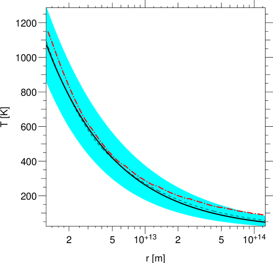
Figure 7: Temperature of the CSE. The solid line represents the best fit (last column in Table. 5) with a unique power-law, the dashed line the best-fit with two power-laws (fourth column in Table 5) and the dot-dashed line the MC results. The shaded region represents the possible domain for a unique power-law by taking into account the errors estimated in Table 3.

The $\chi_{\mathrm{r,min}}^{2}$ values obtained for the two types of temperature parametrisations (one and two power-laws) are quite similar: $0.79$ and $0.73$ respectively. Regarding the data, both temperature parametrisations are indeed acceptable. In addition, these results show that we can actually obtain very good fits from data sets based on more physically consistent scenarios. A complete error analysis and study of the parameter determination has been presented in the previous sections for data generated from FRACS and will not be repeated here. In particular, parameter confidence intervals, from which errors were derived, have already been estimated. Here, we will instead focus on the true errors, i.e. the differences between the true model parameters and the best-fitting values for the parameters (see Table 5). The two types of errors must not be confounded. The true errors reflect the capability of FRACS to mimic the mid-IR interferometric data regarding the information it provides. Of course, with the sparse uv-plane coverage inherent to this kind of data as well as the experimental noise, one should not expect a full agreement of the fitted and the true parameters: they are indeed different.

From Table 5, we see that the geometrical parameters, $\mathrm{PA}_{\mathrm{d}}$, $i$ and $R_{\mathrm{in}}$, can be almost exactly recovered as expected. The source specific intensity $I^{\mathrm{s}}_{\lambda_{0}}$, and the parameters related to the density, $A_{2}$, $n_{\mathrm{in}}$ and $m$ can be recovered fairly well and have best-fitting values close to the true parameters.

The values of $T_{\mathrm{in}}$, $R_{\mathrm{T}}$, $\gamma$ and $\gamma^{\prime}$ reported as “true” in Table 5 are indeed the values of a fit to the average (over the co-latitude for a given $r$) computed temperature in the disc. The true relative differences for $T_{\mathrm{in}}$ do not exceed $7\,\%$ independently of the adopted parameterisation of the temperature (one or two power-laws). The best-fitting values of $\gamma$, the inner temperature gradient, obtained with FRACS are very close to the true values with two and one power-law with true relative error of $1\,\%$ and $7\,\%$ respectively. This already suggests that the mid-IR data provide information on the inner and hottest region of the CSE, in particular on the inner temperature gradient $\gamma$.

Fitting the temperature computed with the MC code with a simple power-law, we obtain $\gamma\simeq 0.64$. This value is close to those of the best fitting models, especially with a unique power-law ($6\,\%$ relative difference). For comparison, the actual mean temperature gradient as derived from the MC simulation is $\simeq 0.60$. For this particular data set, the values of $\gamma^{\prime}$ and $R_{\mathrm{T}}$ recovered by FRACS differ by $28\,\%$ and $45\,\%$ respectively from the actual values. This again confirms the sensibility of the interferometric data to the temperature structure mostly in the inner ($r\la R_{\mathrm{T}}$) regions of the disc. The best-fitting models (fourth and last columns in Table 5) as well as the MC results are shown in Fig. 7. Regarding the errors (estimated from the results given in Table 3) shown as a shaded area, we can see that both temperature parameterisations are essentially the same and show a better agreement with the MC results in the inner than in the outer regions of the disc.

We considered a “truncated” model with two power-laws (with parameter values listed in the third column of Table 5) in which the CSEs emission for $r\geq R_{\mathrm{T}}$, the “outer” regions, has been set to 0. We then compared the visibilities and the fluxes of this truncated model to the same model including the outer region emission. We obtained relative differences, averaged over all considered wavelengths and baselines (Table 1), of $18\,\%$ and $17\,\%$ respectively. These relative differences are larger, but are still close to the noise level. For this reason, one cannot expect to obtain much information on the outer temperature gradient $\gamma^{\prime}$, at least for the particular configuration we considered.

$$\begin{array}[]{cc}\leavevmode\resizebox{227.62204pt}{}{\includegraphics{14511fg09.eps}}&\leavevmode\resizebox{227.62204pt}{}{\includegraphics{14511fg10.eps}}\\ \leavevmode\resizebox{227.62204pt}{}{\includegraphics{14511fg11.eps}}&\leavevmode\resizebox{227.62204pt}{}{\includegraphics{14511fg12.eps}}\\ \leavevmode\resizebox{227.62204pt}{}{\includegraphics{14511fg13.eps}}&\leavevmode\resizebox{227.62204pt}{}{\includegraphics{14511fg14.eps}}\\ \end{array}$$

Figure 8: Evolution of $m$ and $\mathrm{PA}_{\mathrm{d}}$ with the inclination $i$. Left: $\chi_{\mathrm{r}}^{2}$ maps for the couple $m$ and $\mathrm{PA}_{\mathrm{d}}$ ; right: $\chi^{2}$ maps for the couple $m$ and $i$. Contours are drawn for $\chi_{\mathrm{r,min}}^{2}+\Delta\chi_{\mathrm{r}}^{2}$, with $\Delta\chi_{\mathrm{r}}^{2}=0.3,\,1,\,3$. From top to bottom the inclination $i$ takes the value $20\,\degr$, $50\,\degr$ and $90\,\degr$. The results correspond to model 4, 6, and 10. The limits of the maps have been set to $\pm 25\,\%$ of the true values of the parameters.

$$\begin{array}[]{cc}\leavevmode\resizebox{227.62204pt}{}{\includegraphics{14511fg15.eps}}&\leavevmode\resizebox{227.62204pt}{}{\includegraphics{14511fg16.eps}}\\ \leavevmode\resizebox{227.62204pt}{}{\includegraphics{14511fg17.eps}}&\leavevmode\resizebox{227.62204pt}{}{\includegraphics{14511fg18.eps}}\\ \leavevmode\resizebox{227.62204pt}{}{\includegraphics{14511fg19.eps}}&\leavevmode\resizebox{227.62204pt}{}{\includegraphics{14511fg20.eps}}\\ \end{array}$$

Figure 9: $\chi_{\mathrm{r}}^{2}$ maps for the parameters $n_{\mathrm{in}}$, $A_{2}$ and $m$. The results presented here are those of model (a) ($\tau=0.1$, left part) and model (b) ($\tau=1$, right part). Contours are drawn for $\chi_{\mathrm{r,min}}^{2}+\Delta\chi_{\mathrm{r}}^{2}$, with $\Delta\chi_{\mathrm{r}}^{2}=0.3,\,1,\,3$. The three possible maps corresponding to the combination of these parameters are represented. These three parameters are better constrained in model (a).

7 Conclusion

We proposed and described here a new numerical tool to interpret mid-IR interferometric data. Even though we focussed on the special case of circumstellar disc observations, the numerical techniques have been developed with the aim to be as general as possible. The methods we employ rely on both parameterised physical models and the ray-tracing technique. The need for such a tool is evident because the nature of interferometric data imposes an interpretation through a model of the object to obtain any kind of information. On one hand, Monte-Carlo radiative transfer methods require too much computation time to associate the model-fitting to an automatic minimum search method. On the other hand, purely geometrical function fitting (such as ellipses or Gaussians) are too simple to envisage to obtain physical constraints on the observed disc. Hence, a tool like FRACS fills a blank in the model fitting approach for mid-IR interferometric data interpretation. The main advantages of FRACS are its speed and its flexibility, allowing us to test different physical models. Moreover, an exploration of the parameter space can be performed in different manners and can lead to an estimate of the sensitivity of the fit to the different model parameters, i.e. a realistic error estimate.

We applied these techniques to the special astrophysical case of B[e] star circumstellar environments by generating artificial data in order to analyse beforehand what constraints can be obtained on each parameter of the particular disc model in this work. The techniques will then be applied to real interferometric data of a sgB[e] CSE in a sequel to this paper.

We showed in our analysis that the “geometrical” parameters such as $R_{\mathrm{in}}$, $\mathrm{PA}_{\mathrm{d}}$ and $i$ can be determined with an accuracy $\la 15\,\%$. Mid-IR interferometric data give access to a mean temperature gradient: the temperature structure ($T_{\mathrm{in}}$ and $\gamma$) can be very well determined (within $\la 20\,\%$ and $\la 10\,\%$ respectively). It is possible to have access to the central source emission (with an accuracy $\ga 30\,\%$) when it has a significant contribution to the total flux of the object (a few $\%$ are sufficient). The remaining parameters of our disc model, namely $n_{\mathrm{in}}$, $m$ and $A_{2}$ are not very well constrained by MIDI data alone. $n_{\mathrm{in}}$ is at best determined with an accuracy of about $\ga 50\,\%$ in some cases. If $A_{2}$ can be estimated through spectroscopic observations, then the picture about the $n_{\mathrm{in}}$ and $m$ determination improves somewhat.

FRACS can be used mainly for two purposes. First, it can be used by itself to try and determine physical quantities of the circumstellar matter. Admittedly, it is not a self-consistent model, i.e. the radiative transfer is not solved because the temperature structure is parameterised. From the usual habits in the interpretation of interferometric data it is nevertheless a step beyond the commonly use of toy models or very simple analytical models. This approach has indeed been very successful in the millimetric wavelength range (e.g. see Guilloteau & Dutrey, 1998). Second, it can be viewed as a mean to prepare the work of data fitting with a more elaborate model (such as a Monte Carlo radiative transfer code for instance) and to provide a good starting point.

FRACS is a tool that can help in the process of interpreting and/or preparing observations with second-generation VLTI instruments such as the Multi-AperTure mid-Infrared SpectroScopic Experiment (MATISSE) project (Lopez et al., 2006). In this respect, FRACS is not restricted to the mid-IR, and sub-millimeter interferometric data obtained with the Atacama Large Millimeter Array (ALMA) for instance can be tackled.