Optimization-based string method for finding minimum energy path

Abstract

We present an efficient algorithm for calculating the minimum energy path (MEP) and energy barriers between local minima on a multidimensional potential energy surface (PES). Such paths play a central role in the understanding of transition pathways between metastable states. Our method relies on the original formulation of the string method [Phys. Rev. B ${\bf 66}$, 052301 (2002)], i.e. to evolve a smooth curve along a direction normal to the curve. The algorithm works by performing minimization steps on hyperplanes normal to the curve. Therefore the problem of finding MEP on the PES is remodeled as a set of constrained minimization problems. This provides the flexibility of using minimization algorithms faster than the steepest descent method used in the simplified string method [J. Chem. Phys., ${\bf 126}$(16),164103 (2007)]. At the same time, it provides a more direct analog of the finite temperature string method. The applicability of the algorithm is demonstrated using various examples.

I Introduction

The dynamics of complex systems often involve thermally activated barrier-crossing events that allow the system to move from one local minimum of the energy surface to another. At finite temperatures, the total kinetic energy accessible to the system is on the order of $Nk_{\rm B}T$, where $N$ is the number of degrees of freedom, $k_{\rm B}$ is the Boltzmann constant and $T$ is the temperature of the system. However, this huge amount of energy is distributed over the whole system. Consequently, it fails to cross over the free energy barrier (generally an index-1 saddle point) and move to a different basin of attraction. A system can overcome a free energy barrier only when sufficient energy is localized on an activated region of the system. The activated region is the volume of the sample where bond breaking/formation, atomic re-arrangements etc. take place.Dao et al. (2007); Asaro and Suresh (2005) It is of great theoretical and practical interest to develop algorithms that can enable us to efficiently compute the most probable pathways for such transition events. For systems with relatively smooth energy landscapes, it can be shown that the most probable pathways are the minimum energy paths (MEP). Minimum energy paths are physically relevant in the low temperature dynamics of a system and provides information only about the energy barrier involved in a thermally activated event without any consideration of the width of the channel near the saddle point or other entropic effects. Further, at high temperature, the energy surface becomes rugged due to thermal fluctuations and the presence of multiple peaks of $\mathcal{O}\left(k_{B}T\right)$ makes the concept of MEP irrelevant. However in such a scenario the MEP can still correspond to the path with the maximum likelihood.

The problem of finding MEP and the bottlenecks for transition events can be broadly categorized into two classes depending on the initial conditions: (a) when only the initial point is known, and (b) when both the initial and final points on the energy surface are available. In the former case, one can resort to methods like gentlest ascent dynamicsE and Zhou (2011), dimer methodHenkelman and Jónsson (1999), etc. to explore the energy surface. For the second category, the most notable examples include the string methodE et al. (2002, 2007); Maragliano and Vanden-Eijnden (2007); Vanden-Eijnden (2009) and the nudged elastic band methodHenkelman and Jonsson (2000); Henkelman et al. (2000); Sheppard et al. (2008). In this case, we are given the initial and final states of the system, and our aim is to find the MEP connecting these states. Since there can be multiple paths joining the end points, the converged MEP is dependent on the choice of the initial path. In the original string method, a path $\gamma$ evolves as:

$$\dot{\gamma}=-\nabla V\left(\gamma\right)^{\perp}+r\hat{t}$$ (1)

where, $\dot{\gamma}$ is the time derivative of $\gamma$, $\nabla V^{\perp}=\nabla V-\left(\nabla V,\hat{\tau}\right)\hat{\tau}$ is the gradient of the potential perpendicular to $\gamma$, $\hat{\tau}$ is the unit vector parallel to the tangent to $\gamma$ and $r$ is a Lagrange multiplier used to enforce a particular parametrization of the string.

The string method is easy to implement and works well even if the initial and the final states are not local minimum.E et al. (2002) This advantage has led to a class of algorithms called growing string method that have been tested for real systems using quantum mechanical tools.Peters et al. (2004); Quapp (2005); Quapp et al. (2007) Further, if one is solely interested in knowing the free energy barrier and the configuration at the saddle point, the end of the string need not be a local minimum but some intermediate configuration lying in a basin other than that of the initial point.

The string method is based on the idea of moving curves by using a steepest descent-type of dynamics. It should be emphasized that even though the dynamics used in the string method has very strong steepest decent flavor, the method does not amount to minimizing any energy functionals. In order to apply quasi-Newton type of ideas to accelerate the string method, one has to resort to the Broyden formulation for solving coupled system of equations rather than the BFGS type of formulation for optimization.Ren (2002)

We propose a method that reduces the problem of finding MEP to an optimization problem, so that techniques from optimization theory can now be used directly. This prescription is in some ways an improved version of the locally updated planes (LUP) method proposed earlier by Elber and co-workers.Czerminski and Elber (1989); Choi and Elber (1991) In the LUP method, each intermediate configuration along the approximate path is relaxed by confining its motion to a hyperplane. The hyperplanes are selected such that they are perpendicular to the straight line joining the two end points. The LUP method is unstable because - (i) each intermediate configuration is relaxed independently and the algorithm does not prescribe any scheme to make sure that the path is smooth, (ii) the hyperplane selection scheme can result in the formation of kinks if the path has multiple local energy wells, and (iii) since there is no prescribed way to control the separation between the intermediate configurations, the relaxed path can have images clustered around the local minima. These problems severely limit the convergence to the correct MEP in the LUP method.

The finite temperature string (FTS) method is like an expectation-maximization (EM) algorithm for curves.E et al. (2005); Vanden-Eijnden and Venturoli (2009) The current version of the string method is more in line with the spirit of FTS in which the sampling procedure is replaced by the minimization step.

II The method

Given a curve $\gamma$ that joins two points ${\bf{A}}$ and ${\bf{B}}$ on the energy surface, let us parametrize $\gamma$ as $\gamma=\left\{{\bf X}\left(\alpha\right):\;\alpha\in\left[0,1\right]\right\}$ where $\alpha$ is a continuous parameter. When the end points ${\bf{A}}$ and ${\bf{B}}$ lie in different basins of attraction, the curve $\gamma$ will pass through multiple saddle points that are generally the bottlenecks of transition of a system from ${\bf{A}}$ to ${\bf{B}}$. The path $\gamma$ is the MEP if

$$\left({\bf{\nabla}}{V}\right)^{\bot}\left({\bf{X}}\left(\alpha\right)\right)=0$$ (2)

where $(\nabla V)^{\bot}=\nabla V-(\tau,\nabla V)\tau$ is the component of $\nabla V$ normal to the path $\gamma$ and $\tau$ is the unit tangent vector of $\gamma$. If ${\bf{P}}\left(\alpha\right)$ is the hyperplane perpendicular to the path $\gamma$ at ${\bf{X}}\left(\alpha\right)$, then (2) can be restated as

$${\bf{X}}\left(\alpha\right)={\rm argmin}\left.{V}\right|_{{\bf{P}}\left(\alpha\right)}$$ (3)

This is a variational characterization of the MEP. The new version of the string method is based on the variational formulation in $\left(\ref{MEP2}\right)$. The initial guess path is first discretized to give $\left\{{\bf{X}}_{j}^{0}\right\}_{j=1,\cdots,N}$. At step $m$, the path is updated by the following procedure:

1. Minimization: a number of minimization steps are performed on the hyperplanes normal to the curve at the discretization points. This gives $\left\{{\bf{X}}_{j}^{*}\right\}_{j=1,\cdots,N}$.

2. Mixing: a mixing scheme is applied to get

   $$\tilde{\bf{X}}_{\rm j}={\bf{X}}_{\rm j}^{\rm m}\left(1-\lambda\right)+\lambda{\bf{X}}_{\rm j}^{\ast}$$ (4)

   where, $\lambda\in\left(0,1\right)$ is the mixing co-efficient. This step helps in stabilizing the scheme.

3. Reparametrization: redistribute the intermediate configurations along the string according to some metric, such as, equal spacing in configuration space, or equal spacing in energy space, etc.

   $$\left\{\tilde{\bf{X}}_{\rm j}\right\}\overset{\rm reparametrize}{---\longrightarrow}\left\{{\bf{X}}_{\rm j}^{\rm m+1}\right\}$$ (5)

These steps are performed until convergence. Step 3 is a standard procedure in the string method and accounts for the displacements parallel to the curve. Steps 1 and 2, are different from the original and simplified string methods.

III Algorithmic details

Step 1: Minimization
The minimization procedure can be implemented in different ways. The energy of each intermediate configuration can be minimized on their respective hyperplanes till convergence or the minimization can be performed only for few steps. Minimization algorithms with better convergence like, FIRE (fast inertial relaxation engine)Bitzek et al. (2006), conjugated gradientNocedal and Wright (2000), limited memory BFGSNocedal and Wright (2000), etc. can be used for this purpose. For the sake of completeness below we present the modified versions of BFGS and FIRE algorithms:
BFGS: Starting with an intermediate configuration at ${\bf x}_{0}={\bf X}_{j}^{0}$ on the path and an approximate Hessian matrix ${\bf H}_{0}=\nabla\nabla V\left({\bf x}_{0}\right)$ at ${\bf x}_{0}$, the BFGS scheme involves the following steps until convergence is achieved :Nocedal and Wright (2000)
(i) obtain a direction ${\bf p}_{k}$: ${\bf H}_{k}{\bf p}_{k}=\nabla{\bf F}\left({\bf x}_{k}\right)$, where ${\bf F}\left({\bf x}_{k}\right)=-\nabla V\left({\bf x}_{k}\right)$. This is performed by obtaining the inverse of ${\bf H}_{k}$ by applying the Sherman-Morrison scheme.
(ii) obtain step size $\alpha_{k}$ along ${\bf p}_{k}$ (line search)
(iii) update image: ${\bf x}_{k+1}={\bf x}_{k}+\alpha_{k}{\tilde{\bf p}}_{k}$, where ${\tilde{\bf p}}_{k}={\bf p}_{k}-\left({\bf p}_{k},{\bf\tau}_{j}\right){\bf\tau}_{j}$ is the projection of the search direction perpendicular to the tangent (${\bf\tau}_{j}$) to the path at ${\bf X}_{j}^{0}$.
(iv) set ${\bf s}_{k}=\alpha_{k}{\bf p}_{k}$ and ${\bf y}_{k}=-\left[\nabla{\bf F}\left({\bf x}_{k+1}\right)-\nabla{\bf F}\left({\bf x}_{k}\right)\right]$.
(v) update Hessian:

$$H_{k+1}=H_{k}+\frac{\mathbf{y}_{k}\mathbf{y}_{k}^{\mathrm{T}}}{\mathbf{y}_{k}^{\mathrm{T}}\mathbf{s}_{k}}-\frac{H_{k}\mathbf{s}_{k}\mathbf{s}_{k}^{\mathrm{T}}H_{k}}{\mathbf{s}_{k}^{\mathrm{T}}H_{k}\mathbf{s}_{k}}.\\$$ (6)

FIRE: Starting with an initial intermediate configuration at ${\bf x}={\bf X}_{j}^{0}$ on the path, the following dynamical system can be used for the constrained minimization:Bitzek et al. (2006)

$$\begin{split}{\bf\dot{x}}&={\bf v}-\left({\bf\tau}_{j},{\bf v}\right){\bf\tau}_{j},\qquad\\ {\bf\dot{v}}&=\frac{1}{m}{\bf F}-\beta{\bf v}+\beta\left|\bf v\right|\hat{\bf F}\\ \end{split}$$ (7)

where, $\tau_{j}$ is the tangent to the path at ${\bf X}_{j}^{0}$, $m$ is the mass and $\beta$ is a parameter. For the intermediate images, the tangent $\tau_{j}$ at ${\bf X}_{j}^{0}$ can be approximated as

$$\tau_{j}=\frac{{\bf X}_{j+1}^{0}-{\bf X}_{j-1}^{0}}{\left|{\bf X}_{j+1}^{0}-{\bf X}_{j-1}^{0}\right|},\qquad j=2,3,...\left(N-1\right)$$ (8)

Step 2: Mixing
During minimization, since each intermediate image is relaxed independently, their relaxation step lengths can vary due to which the path develops kinks and is no longer smooth. This makes the tangent vector inaccurate leading to numerical instability. To overcome this difficulty, in the second step, we use a mixing scheme to have better control over step lengths.

Step 3: Reparametrization
Next, reparametrization is performed in two steps: computing the values of the parameter $\tilde{\alpha}$ and performing interpolation to find the reparametrized intermediate configurations. For parametrization by equal arc length we first obtain the length of the string:

$$L_{j}=L_{j-1}+\left|\tilde{\bf X}_{j}-\tilde{\bf X}_{j-1}\right|$$ (9)

where, $L_{0}=0$ and $j=1,2,\;...,N$. The corresponding normalized parameter is then given by $\tilde{\alpha}_{j}=L_{j}/L_{N}$. Next, using cubic spline interpolation scheme, we obtain the intermediate configuration positions $\left\{{\bf{X}}_{\rm j}^{\rm m+1}\right\}$ that are evenly distributed along the string according to the updated parameter $\alpha_{j}=j/N$. For computational efficiency, reparametrization may not be enforced at each step. In fact, we have found that reparametrization is much less important for this version of the string method than the original version.E et al. (2002, 2007) Thus, by constraining the minimization on the normal hyperplanes, we have already removed the strong tendency for the intermediate positions to move towards the local minima. So reparametrization only plays a minor role here for improving the accuracy by optimizing the distribution of the points along the curve.

Naturally one is interested in a comparison of the performance of this version of the string method with the older version. The answer is that it depends on the problems one needs to deal with. Suffice to say that the current version provides an alternative. In addition, this current version of the string method is much closer in spirit to the finite temperature string method in which the minimization step is replaced by a sampling step.E et al. (2005)

IV Illustrative Examples

IV.1 Two-dimensional potential

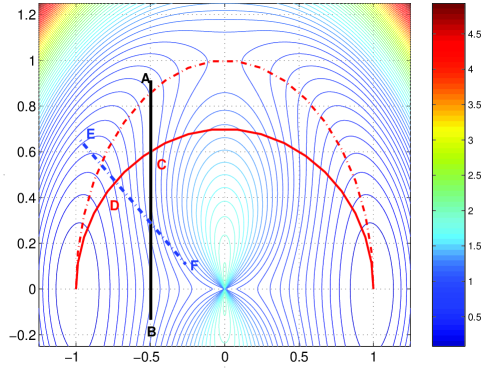
Figure 2: Contour plot of the two-dimensional potential energy landscape showing the MEP (red-dashed curve) and an unrelaxed path (red curve) joining the two local minimum points (-1,0) and (1,0). Lines AB and EF show the different possibilities of selecting hyperplanes at points C and D, respectively, on the string.

To get a better understanding of the effectiveness of the selection of hyperplanes, let us look at the potential energy surface of a simple two-dimensional toy problem shown in Fig. 2. The potential energy is given byE et al. (2007)

$$V\left(x,y\right)=\left(1-x^{2}-y^{2}\right)^{2}+\frac{y^{2}}{x^{2}+y^{2}}$$ (10)

The line AB is perpendicular to the line joining the two local minimum points (-1,0) and (1,0). C is at the intersection of the initial guess path and AB. If we perform a constrained relaxation of C along AB, there are more than one local minimum points in the vicinity. Consequently, during subsequent iterations the intermediate configuration can flip between these locally stable structures. This will make the string uneven leading to the development of kinks due to which it can not converge to the MEP.

However, consider now the line EF which is normal to the path at D. Now the point D has only one choice to lower the energy - go from D towards E, because going towards F means going uphill which increases the energy. Clearly, constrained minimization along hyperplanes normal to the string is a better choice. After relaxation we obtain a smooth string joining the two local minimum points which is shown in Fig. 2 (red dashed curve).

IV.2 Ad-atom diffusion on (111) surface of Cu

Next, we use the optimization-based string method to find the MEP corresponding to rare events taking place in nature. As an example, we study the diffusion of an ad-atom on the $\{$111$\}$ surface of copper. The $\{$111$\}$ surface is used as it has lowest surface energy in Cu. The inter-atomic interactions are modeled using embedded atom method (EAM) potential developed by Mishin et al.Mishin et al. (2001)

On a pure $\{$111$\}$ surface there are multiple sites at which the potential energy is locally minimum. One of them is the face center cubic (fcc) hollow site and the other being the hexagonal close-packed (hcp) hollow site. In a fcc crystal, a set of three $\{$111$\}$ planes forms the stacking sequence while in hcp a set of two $\{$111$\}$ planes forms the stacking sequence. Hence, an ad-atom occupying a surface site which corresponds to fcc (hcp) stacking is called fcc (hcp) hollow site.

The simulation cell contains 512 atoms with cell dimensions of 37.57$\times$20.45$\times$17.71 ${\rm\AA^{3}}$ and cell axes parallel to [111], [1$\bar{1}$0] and [11$\bar{2}$] directions. Periodic boundary conditions are imposed along the [1$\bar{1}$0] and [11$\bar{2}$] directions and free surface conditions are imposed along the [111] direction. The end points of the string are configurations with ad-atoms in hcp hollow sites separated by about 10 $\rm\AA$ on the (111) surface.

Fig. 3 shows the converged MEP (force norm less than 10^-3 eV/$\rm\AA$) as a function of the length of the path in the multidimensional configuration space. The MEP is obtained by performing constrained conjugated gradient minimization on each intermediate configuration. The red curve corresponds to the converged MEP with intermediate configurations evenly distributed (now shown in the figure) along the path. The blue circles denote an intermediate path without reparametrization. The intermediate structures in this case cluster around each other. As shown in the figure, the ad-atom in hcp site is not the lowest energy, the structure with ad-atom occupying the fcc hollow site has lower energy ($\sim$0.004 eV). The diffusion barrier from hcp hollow site to fcc hollow site is 0.036 eV. Similarly, the diffusion barrier from fcc to hcp hollow site is about 0.04 eV. The results shown are without any mixing scheme to update the image positions, i.e. $\lambda$ = 1.

IV.3 Dislocation nucleation in a nano-wire

Understanding the process of dislocation nucleation and multiplication is central to our understanding of structural stability of materials. A dislocation is a line defect which corresponds to the interface between the sheared and unsheared regions of a sample. A bulk sample in nature generally has an astronomical number of defects, of varied dimensionality, present in them. In contrast, in materials of small volume the density of defects can be very small. Small volume materials, such as, quantum dots, nano-wires, thin films, nanostructured materials, etc. have much higher surface area (or grain boundary area) to volume ratio than their bulk counterpartsHemker and Nix (2008); Yip (1998) and defect nucleation from the surface becomes an important driving force for plastic deformation. Given the contrasting length-scales involved, the deformation mechanisms changes from bulk-dominated plasticity to surface-dominated plasticity with decrease in characteristic length scales. One such potentially important form of deformation in nano-wires, nano-pillars, etc. that can play a critical role in controlling plastic deformation is dislocation nucleation.Rabkin and Srolovitz (2007); Hyde et al. (2005); Shan et al. (2008) Here, we perform atomistic simulations of heterogeneous dislocation nucleation in a Cu nano-wire. We use a nano-wire of square cross-section to include the corner as a preferential nucleation site.

The simulation cell has 28,900 atoms and the cell dimensions are 90.375$\times$90.375$\times$90.375 $\rm\AA^{3}$. The cell axes are parallel to [100], [010] and [001] directions. Periodic boundary conditions are maintained along [001] direction (i.e. wire axis) and free surface conditions are imposed along the remaining two directions. The interatomic interactions are modeled using embedded atom method (EAM) potential developed by Mishin et al.Mishin et al. (2001) Fig. 6 shows the initial structure of the nano-wire. Central symmetry scheme of coloring is used.Kelchner et al. (1998) The converged MEP (force norm smaller than 10^-3 eV/$\rm\AA$) is obtained by performing constrained conjugated gradient minimization on each intermediate configuration along the path.

The initial structure is a defect-free pure Cu nano-wire and the final structure is one with a dislocation loop (not a local minimum). The initial structure is generated by applying a compressive strain of 6 $\%$ along the nano-wire axis and then performing conjugated gradient relaxation. The final structure with a dislocation loop is generated by applying a relative displacement equal to a partial Burgers vector between two $\{$111$\}$ planes. The initial guess path is generated using linear interpolation between the end point configurations.

Fig. 5 shows a section of the multi- dimensional PES as a function of the distance between the initial point and intermediate configurations. Fig. 6 shows an intermediate configuration close to the saddle point. The activation energy barrier is 0.43 eV and the sheared region consists of around 30 atoms. Central symmetry scheme of coloring is used so only the atoms in the sheared region are visible.Kelchner et al. (1998) More details about the thermally activated nature of dislocation nucleation can be found elsewhere.Zhu et al. (2008)

V Conclusion

In this paper a modified version of the string method is proposed. The proposed method allows determining the MEP by finding the minimum energy configuration along the hyperplanes normal to the path. The algorithm is simple, easy to implement and provides the flexibility of using faster minimization algorithms.

The applicability of the algorithm is demonstrated using a simple two-dimensional potential energy landscape. The algorithm can be easily extended to study systems of higher dimensions. As examples taken from nature, diffusion barriers of an ad-atom on the surface of Cu and the process of heterogeneous dislocation nucleation from the corner of a nano-wire are evaluated. For the ease of reference, codes for some sample problems are placed in a publicly accessed web link.Str

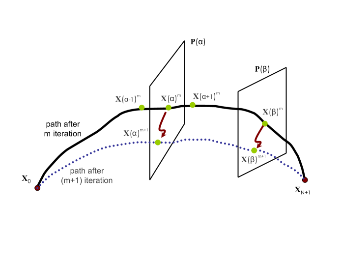
Figure 1: Schematic representation of the optimization-based string method to find MEP. The intermediate configuration at ${\bf{X}}^{m}\left(\alpha\right)$ is relaxed to ${\bf{X}}^{m+1}$ on a plane ${\bf{P}}\left(\alpha\right)$ which is perpendicular to the tangent at ${\bf{X}}^{m}\left(\alpha\right)$.

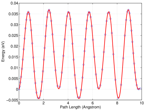
Figure 3: Converged MEP of the ad-atom diffusion on a (111) free surface in Cu. At the end point the ad-atom occupies hcp hollow sites that are about 10 $\rm\AA$ apart. The energy barrier for diffusion from hcp to fcc hollow site is 0.036 eV and from fcc to hcp hollow site is 0.04 eV. The converged MEP is shown in the red-curve while the blue circles show an intermediate path without parametrization.

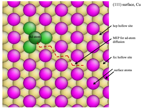
Figure 4: A snapshot of the initial structure of ad-atom on (111) surface of Cu sample. The MEP is shown in red dashed line. Coordination number (CN) coloring is used in this case. The atoms on the free surface have CN 9 while those near the ad-atom have CN 10. The ad-atom sitting on the hcp hollow site has CN 3.

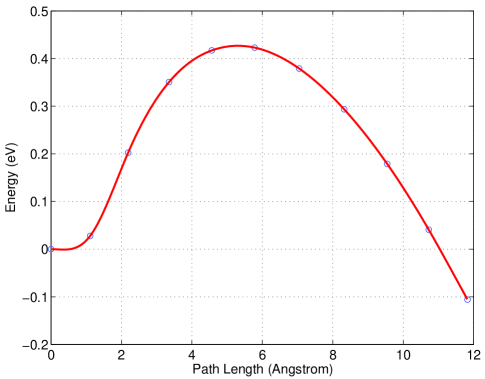
Figure 5: The converged MEP of the heterogeneous dislocation nucleation from the corner of a Cu nano-wire. The zero temperature energy barrier is 0.43 eV for a 6 $\%$ uniaxial compressive strain applied along a direction parallel to the wire axis. The initial state is a defect free Cu nano-wire with (100) surfaces.

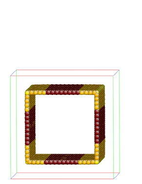
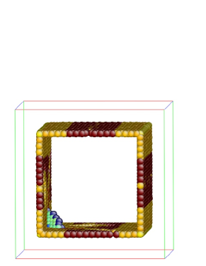
Figure 6: Snapshots of the initial and the saddle configuration for the process of heterogeneous dislocation nucleation from the corner of a nano-wire. The nano-wire is under uniaxial compression of 6 $\%$, the strain axis being parallel to the wire axis. The central symmetry scheme of coloringKelchner et al. (1998) is used: 6 only the atoms on the surface are visible, 6 the surface and the atoms in the sheared region, in the saddle point configuration, are visible. The viewing direction is parallel to the wire axis.