Dynamics of Fluid Mixtures in Nanospaces

Abstract

A multicomponent extension of our recent theory of simple fluids [ U.M.B. Marconi and S. Melchionna, Journal of Chemical Physics, 131, 014105 (2009) ] is proposed to describe miscible and immiscible liquid mixtures under inhomogeneous, non steady conditions typical of confined fluid flows. We first derive from a microscopic level the evolution equations of the phase space distribution function of each component in terms of a set of self consistent fields, representing both body forces and viscous forces (forces dependent on the density distributions in the fluid and on the velocity distributions). Secondly, we solve numerically the resulting governing equations by means of the Lattice Boltzmann method whose implementation contains novel features with respect to existing approaches. Our model incorporates hydrodynamic flow, diffusion, surface tension, and the possibility for global and local viscosity variations. We validate our model by studying the bulk viscosity dependence of the mixture on concentration, packing fraction and size ratio. Finally we consider inhomogeneous systems and study the dynamics of mixtures in slits of molecular thickness and relate structural and flow properties.

I Introduction

In recent years, the experimental study of the flow of liquids in nanometric structures has become an important and rapidly evolving discipline driven by technological applications, such as lab-on-a-chip systems, electrophoresis and electro-osmotic pumping. The mixing and separation of different molecules according to their size or chemical and transport properties is a major issue in chromatography, nanofluidic logic gates and electrokinetics. Many applications are foreseen also in biotechnologies, because very small quantities of liquid components are sufficient for analysis and synthesis, including the possibility of isolating and analyzing or manipulating a single molecule in a single nanochannel or surface with nanoscale features sparreboom ; schoch .

These technological advances require a better theoretical understanding of the fluid properties in confined geometries and under non-equilibrium conditions. At the nanoscale, new areas of physics, chemistry and materials science come in. The systems become more surface-like and molecules never explore a bulk-like environment and because inhomogeneities have a great impact some interesting phenomena arise. Whereas a large body of information has been accumulated in the last thirty years concerning the physics of inhomogeneous fluids under thermodynamic equilibrium conditions Evans2 , the state of the art of flowing fluids is not so advanced nicholson ; aiche ; majumder ; rauscher .

It is crucial to understand how the interplay between the various forces occurs and how it changes when going from macrosystems to nanosystems. It is clear from dimensional considerations that the relative importance of forces changes with the typical dimensions of the systems and we expect that the smaller the sample under scrutiny the more important the role of surface forces is. Not only nanoscale flows are dominated by viscous effects if turbulence is absent, but wherever frequent molecule-channel wall collisions occur besides molecule-molecule collisions, we expect a modified frictional resistance Guo1 .

The generalization of fluid dynamics from pure to multicomponent fluid mixtures composed of different components or species requires the introduction of some new concepts. While traditional computational fluid methods involve some ad hoc extrapolation of Navier-Stokes equation to confining geometries, our approach is based on a microscopic kinetic equation incorporating the effects of the inhomogeneities in its structure.

The major difference with respect to one-component fluids is the phenomenon of concentration diffusion. We shall study a multicomponent kinetic equation Chapman ; Degroot ; Pina ; Ferziger ; Tham that has been considered in the past by several authors with the specific goal of computing the transport coefficients from a microscopic approach. Many of these studies, which were based on the Boltzmann equation or on its extension to the dense case, the Boltzmann-Enskog equation, require some analytical and numerical effort, so that a simpler treatment of the interactions has been proposed. A very popular approximation is represented by the phenomenological Bhatnagar-Gross-Krook (BGK) equation whose merit is to reduce the complexity of the original Boltzmann collision kernel $\Omega^{\alpha\beta}$ between species $\alpha$ and $\beta$ by introducing a simple relaxation-time ansatz BGK ; Gross ; Garzo ; Andries ; Sofonea . The BGK, in spite of being even less accurate than the original Boltzmann equation, has enjoyed a great popularity especially in conjunction with the Lattice Boltzmann method (LBM) thanks to the simplicity of the collision kernel leading to a considerable speed-up of the numerics LBgeneral .

However, in the multicomponent case the choice of the form of the BGK relaxation term is not unique and hard to infer from the original $\Omega^{\alpha\beta}$, and the literature abounds of several proposals Hamel ; Luo ; Zhaoli ; Asinari ; Xu .

In order to describe with sufficient accuracy the fluid structure at length scales comparable with the size of the particles we shall resort to methods similar to those of density functional theory (DFT) employed in the study of equilibrium and non equilibrium properties Evans1 ; Tarazona ; ArcherEvans ; Lowen . In the case of hard-core fluids, DFT and its dynamical extension gives excellent results and can be extended to more realistic fluids by using the van der Waals picture of decomposing the total inter-particle potential into a short-range repulsive potential and a long-range attractive potential tail. The first is treated by means of a reference hard-sphere system whilst the second is considered within the random phase approximation (RPA). Such a decomposition can describe phase separating systems, wetting phenomena, two phase interfaces, but predicts transport coefficients of purely hard-core systems Espanol .

The hard-core part of the interaction is treated within the revised Enskog theory (RET) vanbeijeren that considers the non-local character of the momentum and energy transfer and takes into account the static spatial correlations among particles. This level of theory does not incorporate the time correlations which are responsible for memory effects and hydrodynamic contributions to the transport coefficients Sung .

With respect to the dynamical DFT umbmnogalilei ; Cecconi , the present theory preserves Galilei invariance and therefore displays full hydrodynamic behavior in the limit of slowly varying fluctuations about the equilibrium reference state.

With the aim of deriving a practical numerical approximation to study mixtures in inhomogeneous situations, we extended the method of Dufty and coworkers Brey to the multicomponent case. The method is a compromise between the RET, of which it retains the accuracy as far as the momentum and energy transfer are involved, and the much simpler BGK, which we employ to evolve the non-hydrodynamic moments of the distribution functions Melchionna2008 ; Melchionna2009 ; Lausanne2009 .

The final product of our theory is a coupled system of simplified equations for the density distributions of individual species describing both the streaming and the collisional stages. These equations are solved by an appropriate extension of the LBM algorithm to include both particle-particle interactions and particle-wall interactions. A simple analysis of the equations is used to derive explicit expressions both for equilibrium thermodynamic quantities, such as pressure, compressibility, etc., and for non equilibrium transport coefficients. It is important to stress the difference between the present work and other LBM based approaches for non-ideal fluids, where only attractive interactions are accounted for by the so-called Shan-Chen pseudo-potential, whose justification is purely mesoscopic, while transport coefficients enter as free parameters of the theory shanchen ; Shan .

Interestingly, over two decades ago Davis and coworkers proposed on phenomenological grounds a local average density model (LADM) of viscosity and diffusivity, based on the principle of local averaging of the density over the volume of a hard sphere LADM . The present approach derives similar expressions for the transport coefficients, but differs from the LADM in the way it solves the resulting evolution equations. Pozhar gave a more rigorous foundation to the transport theory in non-uniform systems, but the resulting theory could not be developed into a computationally tractable method Pozhar ; Pozhar2 . In the present work, we claim that our microscopically founded theory lends itself to relatively simple numerical solutions based on the use of the LBM even in the presence of complex geometries. The numerical application regards fluids confined to a spacing of a few monolayers between solid surfaces, where they may behave very differently from bulk conditions and exhibit unusual properties such as a dramatic increase in viscosity.

The paper is organized as follows: in Sec. II we introduce the model and the evolution equations for the individual distribution functions of the multicomponent system. and in Sec. III we discuss the approximations involved in the theory. In Sec. IV we test the predictions of the resulting evolution equations using a simple confining geometry. In Sec. V we validate the resulting equations numerically and simulate the flow of a mixture in narrow channels. Finally in Sec. VI we present our conclusions and perspectives. Two appendices are added to the paper in order to illustrate the relationship between the collision kernel and the non-ideal part of the chemical potential and discuss some technical details related to the discretization procedure.

II Kinetic equations for the distribution functions

We consider a fluid mixture of $N^{\alpha}$ particles of mass $m^{\alpha}$ , with $\alpha=1,M$, where $M$ represents the number of components, mutually interacting with the potentials $U^{\alpha\beta}({\bf r},{\bf r}^{\prime})$. The probability density of finding a particle of type $\alpha$ at position ${\bf r}$ with velocity ${\bf v}$ at time $t$ is proportional to the the single-particle distribution functions, $f^{\alpha}({\bf r},{\bf v},t)$, normalized as follows:

$$N^{\alpha}=\int d{\bf r}\int d{\bf v}f^{\alpha}({\bf r},{\bf v},t).$$ (1)

The evolution of $f^{\alpha}$ is given, in principle, by the exact BBGKY hierarchy of dynamical equations for the reduced distribution functions Chapman , whose first member is the following kinetic equation for the $\alpha$ component:

$$\partial_{t}f^{\alpha}({\bf r},{\bf v},t)+{\bf v}\cdot{\bf\nabla}f^{\alpha}({\bf r},{\bf v},t)+\frac{{\bf F}^{\alpha}({\bf r})}{m^{\alpha}}\cdot\frac{\partial}{\partial{\bf v}}f^{\alpha}({\bf r},{\bf v},t)=\sum_{\beta}\Omega^{\alpha\beta}({\bf r},{\bf v},t),$$

(2)

where ${\bf F}^{\alpha}({\bf r})$ is an external velocity independent force field acting on component $\alpha$ and $\Omega^{\alpha\beta}$ represents the effect of the interactions among the fluid particles of type $\alpha$ and $\beta$. In principle, the exact form of $\Omega^{\alpha\beta}$ is known, but it involves the two-particle distribution functions, which in turn depend on the three particle distribution functions. In order to close this hierarchy different approximations have been proposed, the first historically being the Boltzmann equation expressing $\Omega^{\alpha\beta}$ in terms of products of single-particle distributions. Other specific choices of $\Omega^{\alpha\beta}$ in eq.(2) correspond to different kinds of approximations and lead to equations such as the BGK equation BGK , the Vlasov or RPA equation hansen and the RET equation vanbeijeren .

II.1 Macroscopic variables.

We seek a description in terms of a small number of macroscopic variables which are functions of the fixed position ${\bf r}$ and the time $t$. The procedure leading from eq.(2) to the evolution equations in terms of these variables, closely follows the analysis of the one-component case Melchionna2009 and allows to derive a set of hydrodynamic equations, in the case of a M-component fluid mixture. In $D$ spatial dimensions, there exist $L=(D+M+1)$ conservation laws, for the mass of each species, global momentum and energy. Thus, one can consider the evolution of $L$ linear combinations of velocity moments of $f^{\alpha}$ which are identified with the hydrodynamic fields of the mixture.

In the following, we shall adopt the Einstein summation convention for repeated Cartesian indexes, while sums over components are written explicitly. Let us first write the statistical expressions for the mass density of component $\alpha$:

$$\rho^{\alpha}({\bf r},t)=m^{\alpha}n^{\alpha}({\bf r},t)=m^{\alpha}\int d{\bf v}f^{\alpha}({\bf r},{\bf v},t),$$ (3)

where $n^{\alpha}$ is the associated number density. The total average mass density is given by:

$$\rho({\bf r},t)=\sum_{\alpha}\rho^{\alpha}({\bf r},t),$$ (4)

while the total number density is $n\equiv\sum_{\alpha}n^{\alpha}$. The first velocity moment of the phase-space distribution corresponds to the average local velocity, ${\bf u}^{\alpha}$, of the $\alpha$ component

$${\bf u}^{\alpha}({\bf r},t)=\frac{1}{n^{\alpha}({\bf r},t)}\int d{\bf v}{\bf v}f^{\alpha}({\bf r},{\bf v},t).$$ (5)

We also consider the local barycentric velocity:

$${\bf u}({\bf r},t)=\frac{\sum_{\alpha}\rho^{\alpha}({\bf r},t){\bf u}^{\alpha}({\bf r},t)}{\sum_{\alpha}\rho^{\alpha}({\bf r},t)}$$ (6)

and the so called dissipative diffusion current, measuring the drift component $\alpha$ with respect to the center of mass velocity:

$${\bf J}^{\alpha}({\bf r},t)=\rho^{\alpha}({\bf r},t)[({\bf u}^{\alpha}({\bf r},t)-{\bf u}({\bf r},t)]=\rho^{\alpha}({\bf r},t){\bf w}^{\alpha}({\bf r},t)$$ (7)

and having the property $\sum_{\alpha}{\bf J}^{\alpha}({\bf r},t)=0$.

II.2 Balance equations.

The macroscopic variables $\rho^{\alpha},{\bf u}^{\alpha},{\bf u}$ obey a set of evolution equations derived from eq. (2) as follows. Upon multiplying by $m^{\alpha}$ and integrating over the velocity degrees of freedom both sides of eq. (2) one obtains the continuity equation for the mass density of the species $\alpha$:

$$\partial_{t}\rho^{\alpha}({\bf r},t)=-\nabla\cdot\Bigl{(}\rho^{\alpha}({\bf r},t){\bf u}^{\alpha}({\bf r},t)\Bigl{)}=-\nabla\cdot\Bigl{(}\rho^{\alpha}({\bf r},t){\bf u}({\bf r},t)+{\bf J}^{\alpha}({\bf r},t)\Bigl{)}.$$ (8)

After summing over components, one obtains the global mass continuity equation:

$$\partial_{t}\rho({\bf r},t)+\nabla\cdot\Bigl{(}\rho({\bf r},t){\bf u}({\bf r},t)\Bigl{)}=0.$$ (9)

In establishing eq. (8) we have used the property that the interaction does not affect the partial number densities, i.e. $\int d{\bf v}\Omega^{\alpha\beta}=0$. The momenta of the single species are not locally conserved quantities, due to the interaction between different components. To derive the associated governing equations we first multiply eq. (2) by $m^{\alpha}({\bf v}-{\bf u})$ and then integrate over the velocity with the result:

$$\partial_{t}[\rho^{\alpha}({\bf r},t)u^{\alpha}_{j}({\bf r},t)]+\nabla_{i}\Bigl{(}\rho^{\alpha}({\bf r},t)u^{\alpha}_{i}({\bf r},t)u^{\alpha}_{j}({\bf r},t)-\rho^{\alpha}({\bf r},t)w^{\alpha}_{i}({\bf r},t)w^{\alpha}_{j}({\bf r},t)\Bigl{)}=$$

$$-\nabla_{i}\pi_{ij}^{\alpha}+\frac{F^{\alpha}_{j}({\bf r})}{m^{\alpha}}\rho^{\alpha}({\bf r},t)+\sum_{\beta}C^{\alpha\beta}_{j}({\bf r},t).$$ (10)

In analogy with pure fluids, in eq. (10) we have introduced the kinetic contribution to the partial stress tensor:

$$\pi_{ij}^{\alpha}({\bf r},t)=\rho^{\alpha}({\bf r},t)<(v_{i}-u_{i})(v_{j}-u_{j})>=m^{\alpha}\int d{\bf v}(v_{i}-u_{i})(v_{j}-u_{j})f^{\alpha}({\bf r},{\bf v},t).$$ (11)

Notice that in order to ensure that $\pi_{ij}^{\alpha}$ is independent of a superimposed uniform translation of the entire flowing fluid its definition contains the difference $(v^{\alpha}_{i}-u_{i})$. In eq. (10) we have also defined the projection of the collision term onto the velocity:

$${\bf C}^{\alpha\beta}({\bf r},t)=m^{\alpha}\int d{\bf v}{\bf v}\Omega^{\alpha\beta}({\bf r},{\bf v},t),$$ (12)

representing the contribution to the stress tensor arising from interactions. This integral will be explicitly computed in Sec. III.1 for a specific model. Finally, the term $\rho^{\alpha}w_{i}^{\alpha}w_{j}^{\alpha}$ in the l.h.s. of eq. (10), has nothing to do with viscous effects, but represents an additional stress of dynamical origin due to the different average velocities of the two components Ramshaw and vanishes in the pure fluid. Summing over species eq. (10) we obtain the local conservation law for the total momentum, $\rho{\bf u}$,

$$\partial_{t}[\rho({\bf r},t)u_{j}({\bf r},t)]+\nabla_{i}\left(\rho({\bf r},t)u_{i}({\bf r},t)u_{j}({\bf r},t)]\right)$$

$$=-\nabla_{i}\pi^{(K)}_{ij}+\sum_{\alpha}\frac{F^{\alpha}_{j}({\bf r})}{m^{\alpha}}\rho^{\alpha}({\bf r},t)+\sum_{\alpha\beta}C^{\alpha\beta}_{j}({\bf r},t)$$ (13)

with the total kinetic component of the stress tensor given by:

$$\pi^{(K)}_{ij}({\bf r},t)=\sum_{\alpha}\pi^{\alpha}_{ij}({\bf r},t).$$ (14)

The set of eqs. (8) and (13) is not determined unless additional relations specifying the pressure tensor (14) in terms of the selected macroscopic fields are given. Hydrodynamics at the Navier-Stokes level closes the equations by assuming a simple linear relation between fluxes and derivatives of the fields via phenomenological transport coefficients (such as the viscosity and conductivity) whose values are not known a priori, but which must be taken from experiments. Kinetic theory, working at the level of the non-equilibrium distribution functions, avoids such assumptions.

III Simplified kinetic model

In a nutshell, our strategy consists in solving the kinetic equations rather than the balance equations (8) and (13). It involves concepts borrowed from the lattice Boltzmann method (LBM) and from density functional theory (DFT). The LBM can be regarded as an efficient approach to treat inhomogeneous systems and multiphase flows and provides an alternative to the solution of the Navier-Stokes equations. Conditions at solid boundaries are relatively easily implemented using the LBM, making it well suited for handling complex geometries. The LBM becomes particularly useful to treat non-local effects, such as wetting layers, interfaces, layering etc., if used in conjunction with a simplified kinetic approach suggested by Dufty and coworkers in the case of one-component fluids Brey .

To introduce the simplified kinetic model for mixtures, we refer to ref. Melchionna2009 , where we discussed the simpler one-component case and reduced the full transport equation (2) to a simpler form. The extension to the multicomponent case requires some subtleties which are needed in order to satisfy a key requirement of this approximation: the modified kinetic equation and the original one must share the same equations for the partial densities and momenta, i.e. the distributions must have the same low order projections. Doing so, we are able to treat exactly the contribution of the collision operator to the hydrodynamic equations. As a result, we need to make approximations only on that part of the collision operator which acts on the higher order, non-conserved modes. This latter contribution can be handled in the spirit of some cruder approximation, such as the BGK-like approximation Sofonea . Since the velocity distributions in the final equilibrium state are known it is easy to construct the BGK collision operator in such a way that it verifies some basic properties of the original problem, namely particle and momentum conservation. Our two-component extension of the simplified kinetic equation reads:

$$\partial_{t}f^{\alpha}({\bf r},{\bf v},t)+{\bf v}\cdot{\bf\nabla}f^{\alpha}({\bf r},{\bf v},t)+\frac{{\bf F}^{\alpha}({\bf r})}{m^{\alpha}}\cdot\frac{\partial}{\partial{\bf v}}f^{\alpha}({\bf r},{\bf v},t)$$

$$=\frac{1}{k_{B}T}\frac{\psi^{\alpha}({\bf r},{\bf v},t)}{n^{\alpha}({\bf r},t)}({\bf v}-{\bf u})\cdot\sum_{\beta}{\bf C}^{\alpha\beta}({\bf r},t)-\omega[f^{\alpha}({\bf r},{\bf v},t)-\psi^{\alpha}_{\perp}({\bf r},{\bf v},t)],$$

(15)

where $\omega$ is a collision frequency which depends on the two species and

$$\psi^{\alpha}({\bf r},{\bf v},t)\equiv n^{\alpha}({\bf r},t)[\frac{m^{\alpha}}{2\pi k_{B}T}]^{3/2}\exp\Bigl{(}-\frac{m^{\alpha}({\bf v}-{\bf u}({\bf r},t))^{2}}{2k_{B}T}\Bigl{)}$$ (16)

and

$$\psi^{\alpha}_{\perp}({\bf r},{\bf v},t)\equiv\psi^{\alpha}({\bf r},{\bf v},t)\Bigl{\{}1+\frac{m^{\alpha}({\bf u}^{\alpha}({\bf r},t)-{\bf u}({\bf r},t))\cdot({\bf v}-{\bf u}({\bf r},t))}{k_{B}T}\Bigl{\}}.$$

(17)

The proposed form (15) differs from the existing literature about mixtures in a few aspects. In the first place, the mixtures were treated either by including the full collision operator or by assuming the BGK to be a valid replacement. The simplified kinetic method, to the best of our knowledge, was never applied to mixtures. Our choice for the BGK term is based on a single relaxation time for the two components and represents perhaps the minimal model satisfying the conservation laws compatible with the Dufty and coworkers strategy.

A few comments are in order. First of all, eqs. (8), (10) and (13) are immediately recovered after multiplying eq. (15) by $m^{\alpha},m^{\alpha}({\bf v}-{\bf u})$ and integrating over the velocity, ${\bf v}$. Second, the coupling between the evolution equations of the two distributions $f^{\alpha}$ occurs through the nonlinear collision kernel and this fact is also reflected in the BGK representation of that kernel. Equation (2) contains two terms $\Omega^{\alpha\beta}$, one for each type of interaction, but in the modeling of the BGK relaxation time approximation it is convenient to choose a single collision term. This assumption is valid not only because the coupling between the two distributions is achieved via the barycentric velocity ${\bf u}$ contained in $\psi^{\alpha}$, but also through the term ${\bf C}^{\alpha\beta}$. Third, the classical BGK approximation when applied to a one-component fluid would involve the difference between the distribution $f^{\alpha}$ and the local Maxwellian $\psi^{\alpha}$. In the present case a non exponential prefactor in eq. (17) has been introduced and serves as to ”orthogonalize” the term $\omega[f^{\alpha}-\psi^{\alpha}_{\perp}]$ to the ”true” collisional terms, ${\bf C}^{\alpha\beta}$, so that the BGK does not lead to modifications of the hydrodynamic equations. Also notice that the first velocity moment of $\psi^{\alpha}$ is $n^{\alpha}{\bf u}$, whereas the first moment corresponding to $\psi^{\alpha}_{\perp}$ is $n^{\alpha}{\bf u}^{\alpha}$. The present ansatz reduces to our one-component equation Melchionna2009 in the limit $\psi^{\alpha}_{\perp}\to\psi^{\alpha}$. The above choice satisfies the indifferentiability principle which dictates that when all physical properties of the species are identical, the total distribution $f=f^{A}+f^{B}$ obeys the single species transport equation.

III.1 Interactions

We consider the interaction term featuring in eq. (2) which according to the BBGKY hierarchy can be written as

$$\Omega^{\alpha\beta}({\bf r},{\bf v},t)=\frac{1}{m^{\alpha}}{\bf\nabla}_{v}\cdot\int d{\bf v}^{\prime}\int dr^{\prime}{\bf\nabla}_{r}U^{\alpha\beta}({\bf r}-{\bf r}^{\prime})f_{2}^{\alpha\beta}({\bf r},{\bf r}^{\prime},{\bf v},{\bf v}^{\prime},t),$$ (18)

where $f_{2}^{\alpha\beta}({\bf r},{\bf r}^{\prime},{\bf v},{\bf v}^{\prime},t)$ represents the two-particle distribution function and the $U^{\alpha\beta}(({\bf r}-{\bf r}^{\prime})$ are the pair potentials between particles of species $\alpha$ and $\beta$.

In general, the intermolecular potential, $U^{\alpha\beta}$, contains both a repulsive and an attractive contribution. The latter plays a major role in determining the thermodynamic properties of the system. In the following we shall separate the repulsive and the attractive contributions by representing the short range repulsion between the particles through repulsive hard sphere potentials, characterized by the three diameters $\sigma_{AA}$, $\sigma_{BB}$ and $\sigma_{AB}=(\sigma_{AA}+\sigma_{BB})/2$ plus an attractive contribution:

$$\Omega^{\alpha\beta}({\bf r},{\bf v},t)=\Omega^{\alpha\beta}_{rep}({\bf r},{\bf v},t)+\Omega^{\alpha\beta}_{attr}({\bf r},{\bf v},t).$$ (19)

The repulsive part is treated within the following RET approximation Lopezdeharo :

$$\Omega_{rep}^{\alpha\beta}({\bf r},{\bf v}^{\alpha},{\bf v}^{\beta},t)=\sigma_{\alpha\beta}^{2}\int d{\bf v}^{\beta}\int d{\bf k}\Theta({\bf k}\cdot{\bf v}_{\alpha\beta})({\bf k}\cdot{\bf v}_{\alpha\beta})\times$$

$$\{g_{\alpha\beta}({\bf r},{\bf r}-\sigma_{\alpha\beta}{\bf k},t)f^{\alpha}({\bf r},{\bar{\bf v}}^{\alpha},t)f^{\beta}({\bf r}-\sigma_{\alpha\beta}{\bf k},{\bar{\bf v}}^{\beta},t)$$

$$-g_{\alpha\beta}({\bf r},{\bf r}+\sigma_{\alpha\beta}{\bf k},t)f^{\alpha}({\bf r},{\bf v}^{\alpha},t)f^{\beta}({\bf r}+\sigma_{\alpha\beta}{\bf k},{\bf v}^{\beta},t)\},$$ (20)

where ${\bf v}_{\alpha\beta}=({\bf v}^{\alpha}-{\bf v}^{\beta})$, while ${\bar{\bf v}}^{\alpha}$ and ${\bar{\bf v}}^{\beta}$ are scattered velocities given by

$${\bar{\bf v}}^{\alpha}={\bf v}^{\alpha}-\frac{2m^{\beta}}{m^{\alpha}+m^{\beta}}({\bf k}\cdot{\bf v}_{\alpha\beta}){\bf k}$$

$${\bar{\bf v}}^{\beta}={\bf v}^{\beta}+\frac{2m^{\alpha}}{m^{\alpha}+m^{\beta}}({\bf k}\cdot{\bf v}_{\alpha\beta}){\bf k}.$$ (21)

The quantities $g_{\alpha\beta}({\bf r},{\bf r}\pm\sigma_{\alpha\beta}{\bf k})$ are the three hard sphere pair correlation functions evaluated when the particles of species $\alpha$ and $\beta$ are at contact. The RET collisional term describes the large momentum binary exchanges due to close encounters between the cores, whereas the attractive term can be seen as a slowly varying average force, involving small momentum exchanges. In detail, the attractive tails of the potentials are treated in a mean field approximation, rewriting the second term of the r.h.s. of eq.(19) by factorizing the two-particle distribution functions

$$f_{2}^{\alpha\beta}({\bf r},{\bf v},{\bf r}^{\prime},{\bf v}^{\prime},t)\approx g_{\alpha\beta}({\bf r},{\bf r}^{\prime},t)f^{\alpha}({\bf r},{\bf v},t)f^{\beta}({\bf r}^{\prime},{\bf v}^{\prime},t),$$ (22)

that is, by neglecting velocity correlations completely:

$$\Omega^{\alpha\beta}_{attr}({\bf r},{\bf v},t)\approx\frac{1}{m^{\alpha}}{\bf\nabla}_{v}\cdot\int d{\bf v}^{\prime}\int dr^{\prime}{\bf\nabla}_{r}U_{attr}^{\alpha\beta}(({\bf r}-{\bf r}^{\prime})g_{\alpha\beta}({\bf r},{\bf r}^{\prime},t)f^{\alpha}({\bf r},{\bf v},t)f^{\beta}({\bf r}^{\prime},{\bf v}^{\prime},t),$$ (23)

where $g_{\alpha\beta}({\bf r},{\bf r}^{\prime},t)$ is the inhomogeneous the pair correlation function of the reference hard-sphere system. Integrating w.r.t. the velocity, we obtain the RPA approximation for the attractive term:

$$\Omega^{\alpha\beta}_{attr}({\bf r},{\bf v},t)=-\frac{{\bf G}^{\alpha\beta}({\bf r},t)}{m^{\alpha}}\cdot{\bf\nabla}_{v}f^{\alpha}({\bf r},{\bf v},t),$$ (24)

where we introduced the molecular fields

$${\bf G}^{\alpha\beta}({\bf r},t)=-\int dr^{\prime}n^{\beta}({\bf r}^{\prime},t)g_{\alpha\beta}({\bf r},{\bf r}^{\prime}){\bf\nabla}_{r}U_{attr}^{\alpha\beta}({\bf r}-{\bf r}^{\prime}).$$ (25)

In order to evaluate the interaction contribution to the momentum balance equation, we use the definition (12) together with eqs. (20) and (24). After some algebra, using explicitly the collision rules eqs.(21) we obtain the following expression:

$$C^{\alpha\beta}_{i}({\bf r},t)=-2\mu_{\alpha\beta}\sigma_{\alpha\beta}^{2}\int d{\bf v}^{\alpha}\int d{\bf v}^{\beta}\int d{\bf k}\Theta({\bf k}\cdot{\bf v}_{\alpha\beta})({\bf k}\cdot{\bf v}_{\alpha\beta})({\bf k}\cdot{\bf v}_{\alpha\beta}){\bf k}_{i}$$

$$g_{\alpha\beta}({\bf r},{\bf r}+\sigma_{\alpha\beta}{\bf k},t)f^{\alpha}({\bf r},{\bf v}^{\alpha},t)f^{\beta}({\bf r}+\sigma_{\alpha\beta}{\bf k},{\bf v}^{\beta},t)+G_{i}^{\alpha\beta}({\bf r},t)n^{\alpha}({\bf r},t)$$ (26)

where we have introduced the reduced mass $\mu_{\alpha\beta}=\frac{m^{\alpha}m^{\beta}}{m^{\alpha}+m^{\beta}}$. To proceed further, we invoke a local equilibrium approximation and replace the distribution functions within the integrals (26) by local Maxwellians

$$f^{\alpha}({\bf r},{\bf v},t)\simeq\phi^{\alpha}({\bf r},{\bf v},t)\equiv n^{\alpha}({\bf r},t)[\frac{m^{\alpha}}{2\pi k_{B}T}]^{3/2}\exp\Bigl{(}-\frac{m^{\alpha}({\bf v}-{\bf u}^{\alpha}({\bf r},t))^{2}}{2k_{B}T}\Bigl{)}$$ (27)

and perform the integrals involved in eq. (20), by expanding ${\bf u}^{\alpha}({\bf r},t)$ about ${\bf u}(r,t)$. We also expand the functions at point $({\bf r}+\sigma_{\alpha\beta})$ about their values at ${\bf r}$ up to first order in the differences. The procedure is completely analogous to the one followed in ref. Melchionna2009 and leads to the final result:

$${\bf C}^{\alpha\beta}({\bf r},t)=-\sigma_{\alpha\beta}^{2}\int d{\bf k}{\bf k}g_{\alpha\beta}({\bf r},{\bf r}+\sigma_{\alpha\beta}{\bf k},t)n_{\alpha}({\bf r},t)n_{\beta}({\bf r}+\sigma_{\alpha\beta}{\bf k},t)\times$$

$$\Bigl{(}k_{B}T-2\sqrt{\frac{2\mu_{\alpha\beta}k_{B}T}{\pi}}{\bf k}\cdot[{\bf u}^{\beta}({\bf r}+\sigma_{\alpha\beta}{\bf k},t)-{\bf u}^{\alpha}({\bf r},t)]\Bigl{)}+{\bf G}^{\alpha\beta}({\bf r},t)n^{\alpha}({\bf r},t).$$

(28)

III.2 Decomposition of the interaction term into specific force contributions.

It is instructive to rewrite the term featuring in formula (28) as a sum of more specific forces:

$$\sum_{\beta}{\bf C}^{\alpha\beta}({\bf r},t)=n^{\alpha}({\bf r},t)\Bigl{(}{\bf F}^{\alpha,mf}({\bf r},t)+{\bf F}^{\alpha,drag}({\bf r},t)+{\bf F}^{\alpha,viscous}({\bf r},t)\Bigl{)}.$$ (29)

We identify the force, ${\bf F}^{\alpha,mf}$, acting on the $\alpha$ particle at ${\bf r}$ due to the influence of all remaining particles, being the gradient of the so-called potential of mean force:

$${\bf F}^{\alpha,mf}({\bf r},t)=-k_{B}T\sum_{\beta}\sigma_{\alpha\beta}^{2}\int d{\bf k}{\bf k}g_{\alpha\beta}({\bf r},{\bf r}+\sigma_{\alpha\beta}{\bf k},t)n_{\beta}({\bf r}+\sigma_{\alpha\beta}{\bf k},t)+\sum_{\beta}{\bf G}^{\alpha\beta}({\bf r},t)$$ (30)

a drag force with local character:

$$F_{i}^{\alpha,drag}({\bf r},t)=-\sum_{\beta}\gamma^{\alpha\beta}_{ij}({\bf r})[u_{j}^{\alpha}({\bf r})-u_{j}^{\beta}({\bf r})]$$ (31)

and a viscous force of non local character:

$$F_{i}^{\alpha,viscous}({\bf r},t)=\sum_{\beta}\int d{\bf r}^{\prime}H_{ij}^{\alpha\beta}({\bf r},{\bf r}^{\prime})[u^{\beta}_{j}({\bf r}^{\prime})-u^{\beta}_{j}({\bf r})].$$ (32)

We have further defined a friction tensor:

$$\gamma^{\alpha\beta}_{ij}({\bf r})\equiv\int d{\bf r}^{\prime}H_{ij}^{\alpha\beta}({\bf r},{\bf r}^{\prime})$$ (33)

and a viscosity kernel:

$$H_{ij}^{\alpha\beta}({\bf r},{\bf r}^{\prime})\equiv 2\sqrt{\frac{2\mu_{\alpha\beta}k_{B}T}{\pi}}g_{\alpha\beta}({\bf r},{\bf r}^{\prime},t)n^{\beta}({\bf r}^{\prime},t)\delta(|{\bf r}^{\prime}-{\bf r}|-\sigma_{\alpha\beta})\frac{(r^{\prime}-r)_{i}(r^{\prime}-r)_{j}}{|{\bf r}^{\prime}-{\bf r}|^{2}},$$ (34)

whose relation with the transport coefficients will become clear in the following.

The term ${\bf F}^{\alpha,mf}$ is related to the gradient of the excess chemical potential of species $\alpha$, $\mu_{int}^{\alpha}({\bf r})$, due to the interactions among the particles. In Appendix A we show that in the case of slowly varying density profiles one has the result

$${\bf F}^{\alpha,mf}({\bf r},t)=-{\bf\nabla}\mu_{int}^{\alpha}({\bf r},t).$$ (35)

The drag term is proportional to the velocity difference of the two species and is present even in the absence of velocity gradients. The viscous term, on the other hand, is proportional to velocity gradients. We can consider the case ${\bf u}^{A}=const$ and ${\bf u}^{B}=const$ and ${\bf u}^{A}\neq{\bf u}^{B}$ and uniform densities so that the tensor $\gamma^{\alpha\beta}_{ij}$ becomes isotropic

$${\bf F}^{A,drag}({\bf r},t)=-\gamma^{AB}({\bf u}^{A}-{\bf u}^{B}).$$ (36)

By using the definition (33) we obtain

$$\gamma^{AB}=\frac{8}{3}(2\pi\mu_{AB}k_{B}T)^{1/2}\sigma_{AB}^{2}g_{AB}n^{B}.$$ (37)

It is interesting to show how the microscopic viscosity kernel (34) is related to the viscosity coefficient. Let us assume a simple case ${\bf u}^{A}={\bf u}^{B}={\bf u}$ with

$${\bf u}({\bf r},t)=(0,0,u_{z}(x,y))$$ (38)

and uniform densities, $n^{A}$ and $n^{B}$. In this case the only non vanishing component of the viscous force is directed along $z$. After some lengthy, but straightforward algebra (see ref Melchionna2009 ) we obtain:

$$F_{z}^{\alpha,viscous}=\frac{4}{15}\sum_{\beta}\sqrt{2\pi\mu_{\alpha\beta}k_{B}T}n^{\beta}\sigma_{\alpha\beta}^{4}g_{\alpha\beta}\Bigl{(}\frac{\partial^{2}u_{z}}{\partial x^{2}}+\frac{\partial^{2}u_{z}}{\partial y^{2}}\Bigl{)}$$ (39)

which allows to identify the collisional contribution to the shear viscosity coefficient by using the macroscopic relation

$$\sum_{\alpha}n^{\alpha}F_{z}^{\alpha,viscous}=\eta^{(C)}\Bigl{(}\frac{\partial^{2}u_{z}}{\partial x^{2}}+\frac{\partial^{2}u_{z}}{\partial y^{2}}\Bigl{)}$$ (40)

from which we can write the explicit formula:

$$\eta^{(C)}=\sum_{\alpha\beta}\eta^{(C)}_{\alpha\beta}=\frac{4}{15}\sum_{\alpha\beta}\sqrt{2\pi\mu_{\alpha\beta}k_{B}T}n^{\alpha}n^{\beta}\sigma_{\alpha\beta}^{4}g_{\alpha\beta}.$$ (41)

In the case of pure fluids, this expression of the viscosity reduces to the one predicted by Longuet-Higgins Longuet , which is known to describe successfully fluids of hard molecules even when the radial distribution function is momentarily isotropic. In spite of the fact that the trial distributions correspond the the local equilibrium state, the singular nature of the interactions allows a finite flux of momentum. Notice that the RPA attractive term does not contribute to the transport coefficients, but only to the potential of mean force.

III.3 Fischer-Methfessel prescription for the pair correlation functions of a non uniform system.

We have deduced the formulas for the viscosity and drag coefficient in the case of systems of uniform densities. In order to apply our theory to non-uniform cases we need to specify how the pair correlation functions are modified with respect to the bulk. The pair distribution function $g_{\alpha\beta}$ appearing in the above formulas is constructed according to a generalization of the prescription put forward by Fischer and Methfessel (FM) Fischer . One first defines the smeared densities $\bar{n}^{\alpha}({\bf r})$ via a uniform averaging of $n^{\alpha}({\bf r})$ over spheres of volume $V_{\alpha}=\pi\sigma_{\alpha\alpha}^{3}/6$ centered at the point ${\bf R}_{\alpha\beta}$ located between the centers of the two spheres at ${\bf r}_{\alpha}$ and ${\bf r}_{\beta}$, respectively:

$${\bf R}_{\alpha\beta}=\frac{{\bf r}_{\alpha}+{\bf r}_{\beta}}{2}.$$ (42)

The smeared densities are Sokolowski :

$$\bar{n}^{\alpha}({\bf R}_{\alpha\beta})=\frac{1}{V_{\alpha}}\int_{V_{\alpha}}d{\bf r}n^{\alpha}({\bf r}-{\bf R}_{\alpha\beta}).$$ (43)

The contact values of the pair correlation functions are computed using the bulk expressions obtained from an extension Boublik ; Mansoori of the Carnahan-Starling equation to mixtures:

$$g_{\alpha\beta}^{bulk}(\{\xi_{n}\})=\frac{1}{1-\xi_{3}}+\frac{3}{2}\frac{\sigma_{\alpha\alpha}\sigma_{\beta\beta}}{\sigma_{\alpha\beta}}\frac{\xi_{2}}{(1-\xi_{3})^{2}}+\frac{1}{2}\Bigl{(}\frac{\sigma_{\alpha\alpha}\sigma_{\beta\beta}}{\sigma_{\alpha\beta}}\Bigl{)}^{2}\frac{\xi_{2}^{2}}{(1-\xi_{3})^{3}},$$ (44)

where the functions $\xi_{n}$ are evaluated for the values of the smeared densities at point ${\bf R}_{\alpha\beta}$ between the two particles at contact:

$$\bar{\xi}_{n}({\bf R}_{\alpha\beta})=\frac{\pi}{6}\sum_{\alpha}\bar{n}^{\alpha}({\bf R}_{\alpha\beta})\sigma_{\alpha\alpha}^{n}.$$ (45)

The pair correlations at contact are evaluated in the inhomogeneous system using the generalized FM ansatz:

$$g_{\alpha\beta}({\bf r}_{\alpha},{\bf r}_{\beta};|{\bf r}_{\alpha}-{\bf r}_{\beta}|=\sigma_{\alpha\beta})=g_{\alpha\beta}^{bulk}(\{\bar{\xi}_{n}({\bf R}_{\alpha\beta})\}).$$ (46)

From the knowledge of $g_{\alpha\beta}$, one can immediately obtain the equation of state for the mixture:

$$\frac{P}{k_{B}T}=n^{\alpha}+n^{\beta}+\frac{2}{3}\pi\sum_{\alpha\beta}n^{\alpha}n^{\beta}g_{\alpha\beta}^{bulk}\sigma_{\alpha\beta}^{3}.$$ (47)

After having made the connection between the collisional term ${\bf C}^{\alpha\beta}({\bf r},t)$ and the three types of forces acting in the fluid eq. (29), we can use the large body of knowledge accumulated over the last twenty years about entropic forces in multicomponent systems Likos . These forces, for instance, determine an effective attraction towards a flat wall of the particles with the larger radius induced by the presence of the small particles. For similar entropic reasons two large particles immersed in a sea of small particles experience an effective attraction. To the best of our knowledge, the interplay between entropic forces and viscous forces is not very well known and is worth to be explored. As an order of magnitude estimate entropic forced are typically $k_{B}Tn\sigma_{AB}^{2}$, whereas the ratio between viscous forces and entropic forces is $\approx{\bf u}/v_{T}$ with $v_{T}=\sqrt{k_{B}T/\mu_{\alpha\beta}}$.

Although recent versions of equilibrium DFT are more accurate than the FM method, it is more convenient to work within the FM approximation for a series of reasons: a) the FM approximation is very simple as compared to the Rosenfeld Rosenfeld prescription for pair correlations; b) our theory not only requires the effective potential $\nabla\mu_{int}^{\alpha}$, but also the viscous and frictional forces which are not given by the DFT method; c) computationally the FM method is much faster, although it becomes numerically unstable at high packing fractions.

III.4 Numerical validation

We consider a binary mixture of HS with $\sigma_{AA}=4$, $\sigma_{BB}=8$ and composition $X_{A}=n^{A}/(n^{A}+n^{B})$. The first validation of the numerical algorithm, succinctly described in Appendix B, is obtained by calculating the shear viscosity of the binary system and initially subjected to a sinusoidal shear wave of small amplitude in bulk conditions.

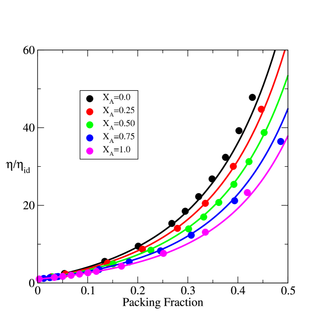
Figure 1: Shear viscosity (normalized to the ideal gas value) versus packing fraction for a bulk mixture at different values of the composition $X_{A}=n^{A}(n_{A}+n_{B})$ of hard spheres of diameter ratio $\sigma_{BB}/\sigma_{AA}=2$ . The viscosity decreases with the concentration $X_{A}$. The continuous curves represent the values obtained with the theoretical formula, whereas the symbols refer to the numerical values obtained from our LBM computer simulations.

The measured decay time is found to have the same temporal decay for both species, and the resulting viscosity curves are reported in Fig. 1. The data are compared with the analytical expression for the decay time obtained by solving the linearized hydrodynamic equations and using the theoretical viscosity of eq. (41). Notice that the viscosity increases monotonically with the packing fraction $\xi_{3}$ of the system and depends on the molar fraction $X_{A}$. At fixed packing fraction, the larger the concentration of the big particles the larger is the viscosity.

The agreement between numerical and analytical data is remarkable. At large packing fraction, a degree of departure from the analytical data indicates the major role played by the collisional integral that apparently is not fully captured by the numerical quadratures. This is an effect of the discretization and of the linear interpolation employed in order to compute some off-lattice points used in the calculation of the surface integrals. From the viewpoint of numerical stability, the range of packing fraction handled in simulation shows that the method is stable up to packing fractions of $\xi_{3}<0.4$, rendering the approach usable in many experimental condensed matter contexts. In proximity of hard walls and under strong flow conditions, the numerical stability range reduces to packing fraction below $\xi_{3}\sim 0.3$.

IV Flow in a slit-like pore. Toy model.

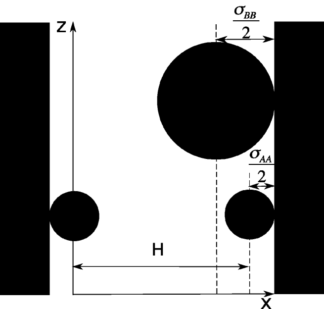
Figure 2: Sketchy view of the system. The walls, parallel to the $yz$ plane are located at positions $x=-\sigma_{AA}/2$ and $x=H+\sigma_{AA}/2$, the flow occurs along the vertical $z$ direction. The direction $y$ is normal to the figure.

We now consider a binary mixture of particles of equal masses and different sizes ($\sigma_{AA}<\sigma_{BB}$) confined in a narrow slit-like pore represented by two parallel smooth plates having infinite area and separated by a distance $H+\sigma_{AA}$ (see fig. 2). The walls are parallel to the $yz$ plane and a flow along the $z$ direction is induced by the presence of a uniform external field, ${\bf F}$, also directed along $z$. Since $H$ is the typical size of the system, $u$ the average flow velocity and $\eta$ the viscosity, the Reynolds number is $Re=\rho uH/\eta$. In the small $Re$ regime, flows have negligible inertia forces. The viscous and pressure forces should be in approximate balance and a reduction, similar to the one occurring between the macroscopic Navier-Stokes and the Stokes equation, takes place also at the present microscopic level of description.

The first remark is that, besides being small in systems of microscopic size and in the limit of low flow velocities, the non linear term in the momentum equation vanishes. In fact, if one imposes the boundary conditions typical of a Poiseuillle flow, in a straight channel, it vanishes due to symmetry.

We rewrite the l.h.s. of eq. (10) as:

$$\partial_{t}[\rho^{\alpha}({\bf r},t)u^{\alpha}_{j}({\bf r},t)]+\nabla_{i}\Bigl{(}\rho^{\alpha}({\bf r},t)u^{\alpha}_{i}({\bf r},t)u^{\alpha}_{j}({\bf r},t)-\rho^{\alpha}({\bf r},t)w^{\alpha}_{i}({\bf r},t)w^{\alpha}_{j}({\bf r},t)\Bigl{)}$$

$$=u^{\alpha}_{j}({\bf r},t)\Bigl{[}\partial_{t}\rho^{\alpha}({\bf r},t)+\nabla_{i}(\rho^{\alpha}({\bf r},t)u^{\alpha}_{i}({\bf r},t))\Bigl{]}+\rho^{\alpha}\Bigl{[}\partial_{t}u^{\alpha}_{j}+u^{\alpha}_{i}({\bf r},t)\nabla_{i}u^{\alpha}_{j}({\bf r},t)\Bigl{]}-\nabla_{i}[\rho^{\alpha}w_{i}w_{j}].$$

The first parenthesis in the r.h.s. is zero due to the continuity equation of species $\alpha$, the second parenthesis is also zero due to the geometry of the problem and the stationarity of the flux, and the last term vanishes because ${\bf w}$ is directed along $z$ and $\rho^{\alpha}$ varies only along $x$.

The flow induced by the presence of uniform fields parallel to the walls is characterized by velocities along the $z$ direction ${\bf u}^{\alpha}=(0,0,u^{\alpha}_{z}(x))$ obeying the following set of stationary equations for each species:

$$\sum_{\beta}\int d{\bf r}^{\prime}H_{ij}^{\alpha\beta}({\bf r},{\bf r}^{\prime})[{\bf u}^{\beta}_{j}({\bf r}^{\prime})-{\bf u}^{\beta}_{j}({\bf r})]-\frac{1}{n^{\alpha}}\nabla_{j}\pi^{\alpha}_{ij}=\nabla_{i}\mu_{int}^{\alpha}({\bf r})+\sum_{\beta}\gamma^{\alpha\beta}_{ij}({\bf r})[{\bf u}^{\alpha}_{j}({\bf r})-{\bf u}^{\beta}_{j}({\bf r})]-F_{i}^{\alpha}.$$

In order to gain insight into the problem, we first set up and solve a toy model, obtained from the full model under some crude approximation. We replace the true non-uniform density profiles by two slabs of constant densities, $n_{A},n_{B}$, respectively:

$$n^{A}(x) = n_{A}\theta(x)\theta(H-x)$$ (49)

$$n^{B}(x) = n_{B}\theta(x-a)\theta(H-a-x).$$

As shown in ref. Melchionna2009 the kinetic contribution to the viscosity due to the individual species is $\eta^{(K)}_{AA}=\frac{k_{B}T}{\omega}n_{A}$, while the collisional part is given by formula (41) . Notice that the above prescription for the kinetic contribution to the viscosity is a consequence of our single time relaxation ansatz. Let us introduce the abbreviations:

$$\eta_{AA}=\Bigl{(}\eta^{(K)}_{AA}+\eta^{(C)}_{AA}\Bigl{)}\,,\qquad\eta_{BB}=\Bigl{(}\eta^{(K)}_{BB}+\eta^{(C)}_{BB}\Bigl{)},\qquad\qquad\tilde{\eta}_{A}=(\eta_{AA}+\eta^{(C)}_{BA})\,,\qquad\tilde{\eta}_{B}=(\eta_{BB}+\eta^{(C)}_{AB}).$$ (51)

When the two species have different diameters, the smaller species can approach the wall up to a distance $\sigma_{AA}/2$, whereas the larger $B$ species can only reach the distance $\sigma_{AA}/2+a$, where $a=(\sigma_{BB}-\sigma_{AA})/2$. In the following, we take $H>2a$ and measure distances, $x$, from the position of closest approach of particles $A$ to the wall as illustrated in Fig. 2.

We now determine the velocity profiles consistent with our toy model. In the central region $a<x<(H-a)$ we obtain the following coupled differential equations for the partial velocities:

$$\eta_{AA}\partial_{x}^{2}u^{A}_{z}(x)+\eta_{AB}\partial_{x}^{2}u^{B}_{z}(x)=\Gamma[u^{A}_{z}(x)-u^{B}_{z}(x)]-F_{z}^{A}n^{A}$$ (52)

$$\eta_{BB}\partial_{x}^{2}u^{B}_{z}(x)+\eta_{AB}\partial_{x}^{2}u^{A}_{z}(x)=-\Gamma[u^{A}_{z}(x)-u^{B}_{z}(x)]-F_{z}^{B}n^{B}$$ (53)

with

$$\Gamma=n^{A}\gamma^{AB}=\frac{8}{3}\sqrt{2\pi K_{B}T\mu_{AB}}\sigma_{AB}^{2}g_{AB}n^{A}n^{B}.$$ (54)

In the excluded layer for the big spheres, that is for $x<a$ or $x>(H-a)$, the equations read:

$$\eta_{AA}\,\partial_{x}^{2}u^{A}_{z}(x)=-F_{z}^{A}n^{A}\,,\qquad u_{z}^{B}(x)=0.$$ (55)

The solution with boundary conditions of zero velocity $u_{z}^{A}$ at $x=0$ and $x=H$, together with zero velocity $u_{z}^{B}$ at $x=a$ and $x=H-a$, and continuous $u^{A}_{z}$ at $x=a$, reads:

$$u^{A}(x)=\frac{F_{z}^{A}n^{A}}{\eta_{AA}}\frac{(H-x)x}{2},\quad x<a,\quad x>(H-a)$$ (56)

while for $a<x<(H-a)$ is given by:

$$u_{z}^{A}(x) = \frac{F_{z}^{A}n^{A}+F_{z}^{B}n^{B}}{\tilde{\eta}_{A}+\tilde{\eta}^{B}}\bigl{(}\frac{(H-x)x}{2}-\frac{(H-a)a}{2}\bigl{)}+C_{A}\bigl{(}\cosh(\lambda(x-H/2))-\cosh(\lambda(a-H/2))\bigl{)}$$ (57)

$$+ \frac{F_{z}^{A}n^{A}}{\eta_{AA}}\frac{(H-a)a}{2}$$

and

$$u_{z}^{B}(x)=\frac{F_{z}^{A}n^{A}+F_{z}^{B}n^{B}}{\tilde{\eta}_{A}+\tilde{\eta}^{B}}\Bigl{(}\frac{(H-x)x}{2}-\frac{(H-a)a}{2}\Bigl{)}+C_{B}\bigl{(}\cosh(\lambda(x-H/2))-\cosh(\lambda(a-H/2))\bigl{)}$$ (58)

with

$$\lambda^{2}=\Gamma\Bigl{(}\frac{\tilde{\eta}_{A}+\tilde{\eta}_{B}}{\eta_{BB}\eta_{AA}-(\eta_{AB})^{2}}\Bigl{)}$$ (59)

and

$$C_{A}=\frac{\tilde{\eta}_{B}}{\tilde{\eta}_{A}+\tilde{\eta}_{B}}\Bigl{(}\frac{1}{\Gamma}\frac{F_{z}^{A}n^{A}\tilde{\eta}_{B}-F_{z}^{B}n^{B}\tilde{\eta}_{A}}{\tilde{\eta}_{A}+\tilde{\eta}_{B}}+\frac{F_{z}^{A}n^{A}}{\eta_{AA}}\frac{(H-a)a}{2}\Bigl{)}\frac{1}{\cosh(\lambda(a-H/2))}$$ (60)

$$C_{B}=-\frac{\tilde{\eta}_{A}}{\tilde{\eta}_{B}}C_{A}.$$ (61)

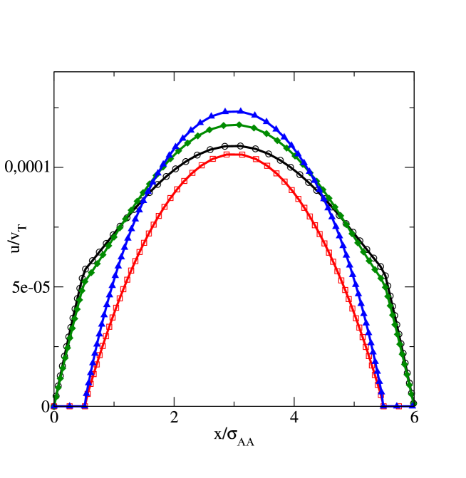
Figure 3: Velocity profiles of the two species for a channel of width $H=6\sigma_{AA}$ and load $F=0.001k_{B}T/\sigma_{AA}$, according to the toy model. The ratio of the diameters of the spheres $\sigma_{BB}/\sigma_{AA}=2$. Velocity of species A (open black circles) and of species B (red squares) at bulk composition $X_{A}=0.25$ and packing fraction $\xi_{3}=0.084$. Velocity profile of species A (green diamonds) and of species B (blue triangles ) at bulk composition $X_{A}=0.75$ and packing fraction $\xi_{3}=0.073$.

The main result of this illustrative model is the presence of different velocity profiles for the two species. The velocity profile of the bigger particles is generally lower than the corresponding profile of the smaller particles, because B effectively sees a narrower slit, so that the confinement effect resulting in a Poiseuille parabolic-like profile is more relevant than for the other species. The velocity difference between species remains finite in the center of the pore. Fig. 3 displays the velocity profiles of the two components for two different values of the composition and at low packing fraction. We will see below that even such a simplified model is able to capture some important features which are better studied by means of our full numerical method.

V LBM numerical results

In the present section we solve numerically the equations for the phase space distributions and study the associated steady state properties. The most interesting applications of our method are those which regard truly inhomogeneous situations where one observes the interplay between the microscopic structure and the flow properties. The small amount of material in the confined region makes experimental probing of confined fluid extremely difficult and thus numerical methods are welcome.

V.1 Profiles.

We reconsider the Poiseuille problem of the previous section using the full power of our theory to obtain the density and velocity profiles of the two components when a uniform field parallel to the plates is applied.

The available region for each hard sphere can be computed according to the density profiles that show where the centers of the spheres can range. Given that the sphere radii are multiples of the mesh spacing, the extrema of the available region can only fall on a mesh point. In this respect, the values of $H$ are equal to $7,13$ and $29$ mesh-points for the three channels, that is $H/\sigma_{AA}=1.75,3.25$ and $7.25$ respectively. On the other hand, for the velocity profiles, we have added a mesh spacing on the left and right extrema to account for the non-slip boundary condition as imposed via the bounce-back scheme in the numerical method. When looking at the intervals from the velocity point of view, they look wider.

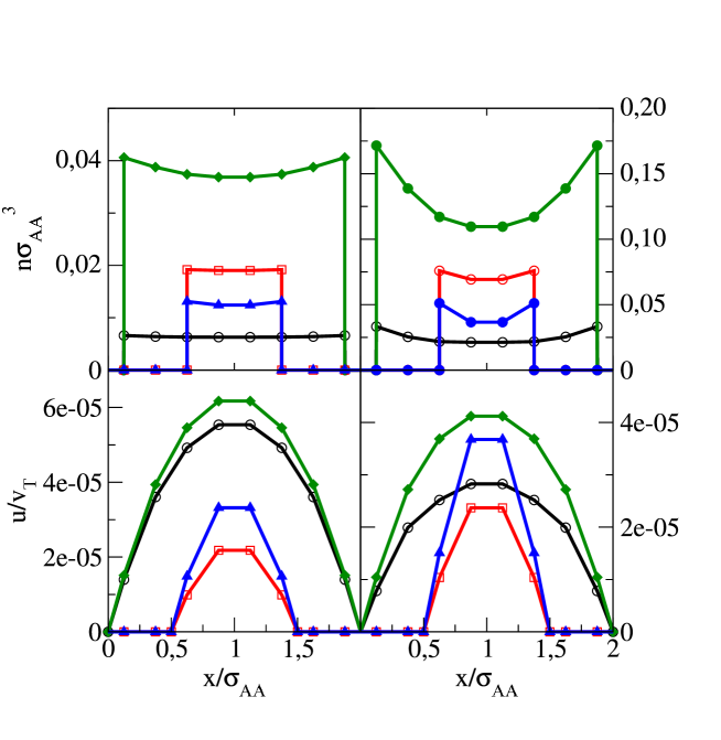
Figure 4: Numerical results for a channel of width $H/\sigma_{AA}=1.75$ and load $F=10^{-6}k_{B}T/\sigma_{AA}$. The spheres ratio of diameters is $\sigma_{BB}/\sigma_{AA}=2$. Upper left panel: Density profile of species A (open black circles) and of species B (red squares) at bulk composition $X_{A}=0.25$ and packing fraction $\xi_{3}=0.084$. Density profile of species A (green diamonds) and of species B (blue triangles ) at bulk composition $X_{A}=0.75$ and packing fraction $\xi_{3}=0.073$. Lower left panel: Velocity of species A (open black circles) and of species B (red squares) at bulk composition $X_{A}=0.25$ and packing fraction $\xi_{3}=0.084$. Velocity profile of species A (green diamonds) and of species B (blue triangles ) at bulk composition $X_{A}=0.75$ and packing fraction $\xi_{3}=0.073$. Upper right panel: Density profile of species A (open black circles) and and of species B (red squares) at bulk composition $X_{A}=0.25$ and packing fraction $\xi_{3}=0.42$. Density profile of species A (green diamonds) and of species B (blue triangles ) at bulk composition $X_{A}=0.75$ and packing fraction $\xi_{3}=0.26$. Lower right panel: Velocity of species A (open black circles) , of species B (red squares) at bulk composition $X_{A}=0.25$ and packing fraction $\xi_{3}=0.42$, velocity of species A (green diamonds) and of species B (blue triangles ) at bulk composition $X_{A}=0.75$ and packing fraction $\xi_{3}=0.26$.

Fig. 4 displays results for the density and velocity profiles for each species in a channel of width $H=1.75\sigma_{AA}$ for a mixture of particles with diameters $\sigma_{AA}=4$ and $\sigma_{BB}=8$ in two different cases: packing fraction $\xi_{3}=0.084$ and composition $X_{A}=0.25$ and packing fraction $\xi_{3}=0.073$ and composition $x_{A}=0.75$. In the upper left panel the mixture is almost a gas and the density profiles for both compositions considered do not display any significant structure, whereas in the lower left panel the velocity profiles have nearly parabolic shapes, each species having its own curvature. One may conclude that in such a regime the flow behavior of the confined fluid is Poiseuille-like. As we increase the packing fraction to $\xi_{3}=0.42$ (composition $X_{A}=0.25$) and packing fraction $\xi_{3}=0.26$ (composition $X_{A}=0.75$), we observe the behavior reported in the right panels of Fig. 4. The large species $B$ is unable to display significant peaks, due to the small plate separation that inhibits the formation of two layers of $B$ particles. The small species, instead, starts developing some density enhancement in the proximity of the walls (upper right panel). The velocity profiles instead still bear a parabolic behavior with the smaller species always being faster than the bigger species.

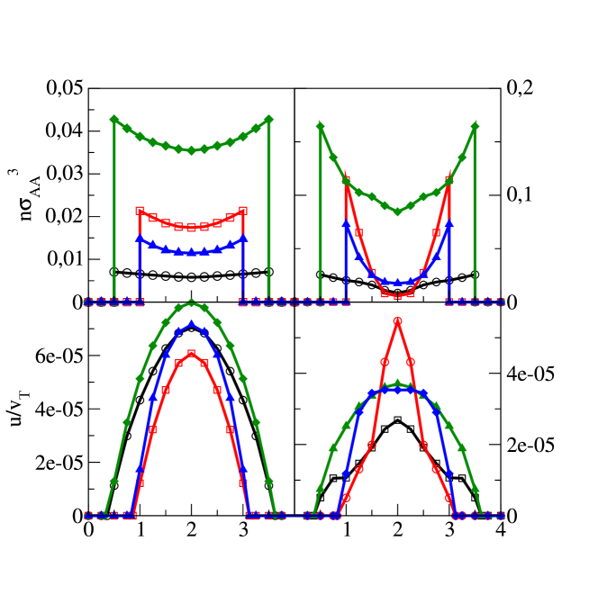
Figure 5: Numerical results for a channel of width $H/\sigma_{AA}=3.25$ and load $F=10^{-6}k_{B}T/\sigma_{AA}$. The ratio of the diameters of the spheres is $\sigma_{BB}/\sigma_{AA}=2$ . The symbols used in the four panels correspond to the same values of packing and concentration as those employed in figure 4.

In Fig. 5 we consider the same state conditions but a wider slit, $H=3.25\sigma_{AA}$, such that more than one layer of particles B can fill the gap. In the low packing region, at $\xi_{3}=0.073$ and at $\xi_{3}=0.084$ (upper left panel), both density profiles are rather flat and the associated velocity profiles do not display significant structure, the smaller particles being faster (lower left panel). As we consider larger packing fractions, $\xi_{3}=0.42$ and composition $X_{A}=0.25$, we observe a stronger structure in the large particles than in the small particles. The other packing fraction, $\xi_{3}=0.26$ (composition $X_{A}=0.75$), also produces some significant peak structure at the walls for the large particles, but the small particles have a rather flat density profile. The small HS are somehow enslaved by the large component as far as the structure is concerned. In the velocity profiles (lower right panel) we observe that the $B$ component for $X_{A}=0.25$ has a higher velocity than the small counterpart near the center-line of the slit. This effect is determined by packing: small particles have more room near the walls while large particles move faster near the center-line.

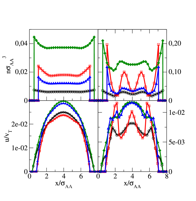
Figure 6: Channel of width $H/\sigma_{AA}=7.25.$ The symbols in the four panels correspond to the same conditions as those employed in figure 4.

In Fig. 6 we consider a channel with $H=7.25\sigma_{AA}$. In the low packing region (left panels), there is not significant structure, the velocity profiles are Poiseuille-like and display the same trend as in the corresponding panel of Figs. 4 and 5. More interesting is the situation at higher packing, shown in the upper right panel. When $\xi_{3}=0.42$ and $X_{A}=0.25$ the large particles display four well defined peaks, while the small particles have a flatter structure. Correspondingly, the velocities of the two species (lower right panel) are anti-correlated with the density profiles, the largest velocities being attained where the density displays local minima. Also the velocity profiles at such large packing fraction show an inversion, that is the larger species has the larger velocity. The other case considered for $\xi_{3}=0.26$, $X_{A}=0.75$ displays a less pronounced structure and nearly no oscillations in the velocity profiles.

To conclude, the density profiles are rather sensitive to the composition and show the characteristic enhancement near the walls as packing increases. On the contrary, we have not found a sensitive dependence of the density profiles on the applied load. The velocity profiles for moderate packing fractions have shapes reminiscent of the parabolic Poiseuille-like profiles, with the velocity of the larger species being smaller at low packing , in agreement with the prediction of the toy model of the previous section.

V.2 Coarse grained observables.

Besides considering the microscopic aspect represented by the various profiles, it is of interest to analyze some average properties, such as the volumetric flow of each component and the selectivity, quantities which are more easily measurable in experiments. We define the volumetric flow rate of each species as:

$$Q^{\alpha}\equiv{\cal A}\int_{0}^{H}dxn^{\alpha}(x)u^{\alpha}(x)$$ (62)

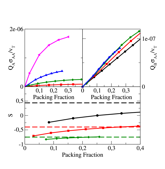
Figure 7: Volumetric flow rates for species A (upper left panel) and B (upper right panel) and selectivity function S (lower panel) as a function of the packing fraction for a channel of width $H=2\sigma_{AA}$ and $X_{A}=0.5$. For the sake of comparison we plotted the lines obtained assuming a simple Poiseuille type of behavior of the system as explained in the text.

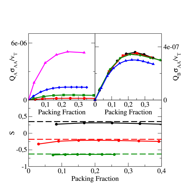
Figure 8: Volumetric flow rates for species A (upper left panel) and B (upper right panel) and selectivity function S (lower panel) as a function of the packing fraction for a channel of width $H=2\sigma_{AA}$ and $X_{A}=0.5$. For the sake of comparison we plotted the lines obtained assuming a simple Poiseuille type of behavior of the system as explained in the text.

where ${\cal A}$ is the area of the plates. In the upper panels of Figs. 7 and 8 we display how these quantities vary with the packing fraction, $\xi_{3}$, for a fixed value of the mixture composition, $X_{A}$. In the lower panel we display how the selectivity, S, defined as

$$S\equiv\frac{Q^{B}-Q^{A}}{Q^{A}+Q^{B}}$$ (63)

varies with the packing at fixed composition.

We first observe that the volumetric flows at low densities increase almost linearly with packing . In general, the volumetric flow of the small species for equal composition ($X_{A}=0.5$) is larger for the small species, on account of the larger effective volume available. If packing increases further, the volumetric flow decreases. Such a feature has the following explanation: in the low density region, $Q^{\alpha}$ increases almost linearly with packing, but as $\xi_{3}$ becomes larger it determines a quadratic increase in viscosity and thus a decrease of the velocity of the fluid in the pore. As a result, there exists an optimal value of the packing for which the volumetric flow is maximum. The peak shifts towards larger values of the packing as the pore becomes larger. Interestingly, such a non-monotonic behavior is captured also by the toy model of section IV . The results suggest that particles could be separated by their size. Hydrodynamic chromatography, instead, exploits the Poiseuille velocity profile in channels rauscher .

VI Conclusions and perspectives

To summarize, we have proposed a new theoretical method to study mixtures under confinement by using concepts derived from both DFT and LBM. The method has been applied to recover bulk properties such as the shear viscosity, and to study inhomogeneous situations, such as the flow in a slit-like channel of molecular thickness. Whereas MD simulations provides a complete microscopic picture for molecular level mechanisms at the price of a demanding computer time, the present method offers an efficient alternative in terms of CPU-time and high numerical versatility.

We have extended the kinetic model described in refs. Brey ; Melchionna2009 to a multicomponent system. The formalism enables us to compute not only the transport coefficients of fluid mixtures, but also to investigate inhomogeneous dynamical properties. We have verified that the numerical solution is in agreement with the values of viscosity predicted by our theory. In addition, we have considered the dynamics of a mixture of particles of different size confined between two parallel plates. Under high confinement, different species display different velocity profiles. We also found non-trivial behavior when the plate separation becomes so narrow that the harshly repulsive forces among the particles and with the confining walls come into play.

We wish to comment that our approach relies on the validity of the local equilibrium approximation and is corroborated by the observation that both local thermodynamic and hydrodynamic theories appear to be reliable up to surprisingly small wavelengths. At smaller scales, both conditions break down and a transition to a genuinely molecular regime takes place. Compared to previous approaches LADM ; Pozhar ; Pozhar2 , our method contains two main ideas which in our opinion render it a workable scheme: the simplified kinetic kernel (15) and the numerical scheme based on the LBM techniques. Very fast numerical solutions can be obtained along these lines and complex geometries can be handled with great simplicity and good analytical insight.

In developing the numerical algorithm via a generalized version of the Lattice Boltzmann method, we did not take into account temperature variations across the system because we wanted to maintain the methodology as simple as possible. The non isothermal extension of the algorithm is doable, but this would require to include Hermite polynomials up to fourth order (that is, 127 mesh neighbors in the collisional part of the algorithm), in order to guarantee numerical stability and physical accuracy. In the future, we plan to handle this aspect.

Before concluding we wish to add that several applications of our theory can be envisaged to the study of fluids in nanospaces. Among others we mention just a few:

a) the spreading of a highly concentrated region in flow conditions and of the competition between the advection and molecular diffusion Bruus ;

b) the transport of different molecular species in a channel of varying width and the influence of the size and/or mass on the dynamical properties rauscher ;

c) the entropic, Asakura-Osawa interactions with walls and the interplay between advection and diffusion. When particles of different size are present one expects that the larger particles experience a larger attraction towards the walls, the so called effective entropic force Evans1999 ; Crocker . At low Reynolds number, the scenario should not be greatly modified, but the issue is worth to be considered with some care;

d) the dynamics of menisci formed in narrow slits between two coexisting liquid phases vanswol ;

e) driven flows past chemically, physically heterogeneous substrates, a mechanism which could enhance mixing Balasz ;

f) since the equilibrium phase diagram of substances under confinement is shifted with respect to bulk conditions, a similar dynamical effect is expected and could be used to obtain specific properties Evans1987 ;

g) cylindrical pores are known to lead to strong, non-trivial size selectivity, which is highly sensitive to the pore width Simonejeanpierre . It would be very interesting to exploit our model in such a geometry.

Appendix A The connection with the chemical potential

In this appendix we give a proof of formula (35). To this purpose let us consider the r.h.s. of the momentum equation (10) for species $\alpha$. At equilibrium the l.h.s. of eq. (10) vanishes together with the drag and the viscous contributions, so that we obtain the condition:

$$k_{B}T{\bf\nabla}n^{\alpha}({\bf r},t)-n^{\alpha}({\bf r},t){\bf F}^{\alpha}({\bf r},t)=n^{\alpha}({\bf r},t){\bf F}^{\alpha,mf}({\bf r},t)$$ (64)

Under the adiabatic hypothesis, we assume the non-equilibrium positional pair correlations to be given by the equilibrium pair correlations Tarazona ; ArcherEvans evaluated when the instantaneous density profiles assume the values $n^{A}({\bf r},t)$ and $n^{B}({\bf r},t)$. The force ${\bf F}^{\alpha,mf}({\bf r})$ can be expressed as

$${\bf F}^{\alpha,mf}({\bf r})=-\int d{\bf r}^{\prime}\sum_{\beta}g_{\alpha\beta}({\bf r},{\bf r}^{\prime})n^{\beta}({\bf r}^{\prime}){\bf\nabla}U^{\alpha\beta}(|{\bf r}-{\bf r}^{\prime}|)$$ (65)

where we have used the property of the hard sphere potential:

$$\int d{\bf r}^{\prime}n^{\beta}({\bf r}^{\prime})g_{\alpha\beta}({\bf r},{\bf r}^{\prime})\nabla_{r}U_{hs}^{\alpha\beta}(|{\bf r}-{\bf r}^{\prime}|)=-k_{B}T\int d{\bf r}^{\prime}n^{\beta}({\bf r}^{\prime})g_{\alpha\beta}({\bf r},{\bf r}^{\prime})\delta(|{\bf r}-{\bf r}^{\prime}|-\sigma_{\alpha\beta})\frac{{\bf r}-{\bf r}^{\prime}}{|{\bf r}-{\bf r}^{\prime}|}$$ (66)

in order to recast the surface integral over the sphere of radius $\sigma_{\alpha\beta}$ eq.(35) into a volume integral. Substituting the result (64) into eq. (65) we obtain the Born-Green-Yvon relation Evans1 . We now compare the r.h.s. of eq. (64) with the exact equilibrium relation

$$k_{B}T{\bf\nabla}n^{\alpha}({\bf r})-n^{\alpha}({\bf r}){\bf F}^{\alpha}({\bf r})=k_{B}Tn^{\alpha}({\bf r})\int d{\bf r}^{\prime}\sum_{\beta}c_{\alpha\beta}({\bf r},{\bf r}^{\prime}){\bf\nabla}^{\prime}n^{\beta}({\bf r}^{\prime})$$

$$=-n^{\alpha}({\bf r}){\bf\nabla}\frac{\delta{\cal F}_{int}}{\delta n^{\alpha}({\bf r})}=-n^{\alpha}({\bf r}){\bf\nabla}\mu_{int}^{\alpha}({\bf r})$$ (67)

where ${\cal F}_{int}$ is the non-ideal contribution to the free energy functional, $-k_{B}Tc_{\alpha\beta}({\bf r},{\bf r}^{\prime})=\frac{\delta^{2}{\cal F}_{int}}{\delta n^{\alpha}({\bf r})\delta n^{\beta}({\bf r}^{\prime})}$ is the Ornstein-Zernike direct correlation function and $-{\bf\nabla}\mu^{\alpha}_{int}$ is the force arising from the interactions with the other fluid particles on a particle located at ${\bf r}$ hansen . By equating the r.h.s. terms of eqs. (65) and (67, we conclude that eq. (35) holds.

Finally, notice that eq. (67) can be rewritten as

$$k_{B}T{\bf\nabla}\ln n^{\alpha}({\bf r})+{\bf\nabla}\mu^{\alpha}_{int}({\bf r})={\bf F}^{\alpha}({\bf r})$$ (68)

that is, in thermal and mechanical equilibrium the net force on a fluid particle at position ${\bf r}$ must vanish. This occurs when the entropic force, represented by the first term, being the resultant of the attractive and repulsive forces exerted on a molecule at ${\bf r}$ from all the other molecules (the second term on the l.h.s.) and the external force (on the r.h.s.) compensate exactly.

Appendix B The discretization procedure

A crucial goal of the present work is to achieve the solution of the coupled integro-differential equations for non-ideal mixtures by means of a suitable numerical scheme. In this work, we consider the Lattice Boltzmann method as the reference framework that enables us to solve the kinetic equation in bulk conditions and under confinement, in particular when the confining geometry is highly non-trivial. The main asset of the LBM is to work directly with the distribution functions by accomplishing a spectral decomposition of the distribution in velocity space via a Hermite representation. In this way, the three-dimensional velocity space is reduced to a handful of sampling points and the three-dimensional real space is discretized over a Cartesian mesh. The resulting distribution function is transformed into a reduced set of populations. The phase space evolution is thus rewritten as an efficient updating algorithm where the streaming operator has the form of a forward Euler updating step. The LBM approach has been previously employed to solve the collisional dynamics of the single-component hard-sphere fluid and provided robust solutions up to packing fraction $<0.35$ Melchionna2009 .

The LBM is a very general framework to handle the evolution of generic kinetic equations and does not depend in any specific way on the form of the collisional kernel LBgeneral . We exploit this generality to solve the collisional dynamics encoded by eq. (15), where non-local structural forces appear as surface integrals, and retain the simple LBM picture of updating the populations. In addition, the BGK kernel of eq. (15) also depends on the Hermite representation via the equilibrium distribution. A second-order expansion of the distribution function, corresponding to a Hermite representation to second order, is usually employed in one-component LBM implementations shanchen ; martys ; heluo ; shanhe .

The distribution function of each species is discretized in velocity space and the continuous phase space distribution is replaced by a $Q$-dimensional array, $f^{\alpha}({\bf r},{\bf v},t)\rightarrow f^{\alpha}_{p}({\bf r},t)$ where $p=1,\dots,Q$ labels discrete velocities ${\bf c}_{p}$. The $Q$ discrete velocities connect neighboring mesh points on a lattice and mirror the hop of particles between mesh points, generally augmented by a null vector ${\bf c}_{0}$ accounting for particles at rest. The form of the lattice velocities ${\bf c}_{p}$ depends on the order of accuracy of the method and reflects into the required Hermite order shanyuanchen .

In essence, the LBM dynamics is achieved by a rearrangement of populations over spatial shifts via an explicit update arising from the following approximation to the streaming operator,

$$\partial_{t}f_{p}({\bf r},t)+{\bf c}_{p}\cdot\partial_{{\bf r}}f_{p}({\bf r},t)\simeq\frac{f_{p}({\bf r}+{\bf c}_{p}\Delta t,t+\Delta t)-f_{p}({\bf r},t)}{\Delta t}$$ (69)

where $\Delta t$ is the time-step. We choose the mesh classified as D3Q19, that is, containing $19$ discrete velocities connecting first and second neighbors of a cubic lattice and overall achieving second-order Hermite accuracy. We choose equal masses for the hard-sphere species so that the thermal velocity is the same for both species and given by $v_{T}=1/\sqrt{3}$. An extension of the present method to different masses can be easily obtained by using the method described in ref. Zhaoli . The updating step for the populations is compactly written as

$$f^{\alpha}_{p}({\bf r}+{\bf c}_{p},t+\Delta t)=\bar{f}^{\alpha}_{p}({\bf r},t)$$ (70)

where ${\bar{f}}^{\alpha}_{p}({\bf r},t)$ is the post-collisional population of species $\alpha$, containing the effect of the BGK relaxation and the hard-core collisions, written as

$${\bar{f}}^{\alpha}_{p}({\bf r},t)={\bar{f}}^{bgk,\alpha}_{p}({\bf r},t)+{\bar{f}}^{hs,\alpha}_{p}({\bf r},t)$$ (71)

The BGK contribution to the post-collisional population has the form

$${\bar{f}}^{bgk,\alpha}_{p}({\bf r},t)=(1-\omega\Delta t)f^{\alpha}_{p}({\bf r},t)+\omega\Delta t\psi^{\alpha}_{\perp,p}({\bf r},t)$$ (72)

where

$$\psi^{\alpha}_{\perp,p}({\bf r},t)=w_{p}n^{\alpha}({\bf r},t)\left[1+\frac{c_{pi}u^{\alpha}_{i}({\bf r},t)}{v_{T}^{2}}+\frac{(c_{pi}c_{pj}-v_{T}^{2}\delta_{ij})\left(v_{T}^{2}\delta_{ij}+2u^{\alpha}_{i}({\bf r},t)u_{j}({\bf r},t)-u_{i}({\bf r},t)u_{j}({\bf r},t)\right)}{2v_{T}^{4}}\right]$$ (73)

and

$$\psi^{\alpha}_{p}({\bf r},t)=w_{p}n^{\alpha}({\bf r},t)\left[1+\frac{c_{pi}u_{i}({\bf r},t)}{v_{T}^{2}}+\frac{(c_{pi}c_{pj}-v_{T}^{2}\delta_{ij})u_{i}({\bf r},t)u_{j}({\bf r},t)}{2v_{T}^{4}}\right].$$ (74)

The $w_{p}$ are the $Q$ weights normalized to unity that arise from the Hermite expansion LBgeneral . Formula (74) is a low-Mach ($O[Ma^{3}]$) expansion of the local Maxwellian corresponding to the barycentric velocity for a mixture of equal masses

$${\bf u}({\bf r},t)={\sum_{\alpha}n^{\alpha}{\bf u}^{\alpha}({\bf r},t)\over\sum_{\alpha}n^{\alpha}({\bf r},t)}$$ (75)

with

$$n^{\alpha}({\bf r},t) = \sum_{p}f_{p}^{\alpha}({\bf r},t)$$

$$n^{\alpha}({\bf r},t){\bf u}^{\alpha}({\bf r},t) = \sum_{p}{\bf c}_{p}f_{p}^{\alpha}({\bf r},t)$$ (76)

The hard-sphere post-collisional contribution is

$${\bar{f}}^{hs,\alpha}_{p}({\bf r},t)=-w_{p}\left[\frac{c_{pi}C^{(\alpha)}_{i}({\bf r},t)}{v_{T}^{2}}+\frac{(c_{pi}c_{pj}-v_{T}^{2}\delta_{ij})u_{i}({\bf r},t)C^{(\alpha)}_{j}({\bf r},t)}{v_{T}^{4}}\right].$$ (77)

The collisional integral is approximated via the following real-space quadrature

$${\bf C}^{(\alpha)}({\bf r},t)=\sum_{\beta}{\bf C}^{\alpha\beta}({\bf r},t)= -4\pi\sum_{\beta}\sigma_{\alpha\beta}^{2}\sum_{q}W_{q}{\bf k}_{q}g_{\alpha\beta}({\bf r}+{1\over 2}\sigma_{\alpha\beta}{\bf k}_{q},t)n_{\alpha}({\bf r},t)n_{\beta}({\bf r}+\sigma_{\alpha\beta}{\bf k}_{q},t)\times$$ (78)

$$\Bigl{(}v_{T}^{2}-2\sqrt{\frac{2v_{T}^{2}}{\pi}}{\bf k}_{q}\cdot[{\bf u}^{\beta}({\bf r}+\sigma_{\alpha\beta}{\bf k}_{q},t)-{\bf u}^{\alpha}({\bf r},t)]\Bigl{)}$$

where ${\bf k}_{q}$ are the nodes of the quadrature over a spherical surface abramovitzstegun and $W_{q}$ the associated quadrature weights. We choose a 18-points quadrature that is exact for quadratic integrands. The quadrature nodes on the unit sphere are the six on-axis points $(\pm 1,0,0)$, $(0,\pm 1,0)$ and $(0,0,\pm 1)$ and twelve points along the diagonals $(\pm\sqrt{2},\pm\sqrt{2},0)$, $(\pm\sqrt{2},0,\pm\sqrt{2})$ and $(0,\pm\sqrt{2},\pm\sqrt{2})$. Correspondingly, the quadrature weights are $W_{q}=1/15$ for the on-axis points and $W_{q}=1/30$ for the diagonal points. It should be borne in mind that the quadrature points do not necessarily fall on the mesh. For instance, if the the HS radius is an integer and one considers intraspecies collisions, there are only six quadrature nodes that fall on the mesh while twelve nodes along the diagonals do not. In order to sample the fluid density and velocity on off-mesh points, we employ a trilinear interpolation scheme NUMRECIPES . It is clear that the accuracy of the collisional integrals improve for larger HS diameters, since the eight mesh points employed in the trilinear interpolation fall closer to the spherical surface. The same type of consideration applies for the interspecies integral and, in all circumstances, for the midpoint rule employed to estimate the radial distribution function via the Carnahan-Starling expression eq. (44). In our numerical applications, we applied a trilinear interpolation for any off-mesh quadrature nodes and midpoints for the radial distribution function, and chose HS diameters to be even numbers in order to minimize the number of off-mesh interpolations.

In solving eq. (15) with the LBM approach, we need to control the numerical error introduced by the discretization procedure over velocity, space and time variables. It is well-known that for one-component, uncorrelated fluids LBM bears three types of error as compared to the analytical solution of the incompressible Navier-Stokes equation. The first error depends on the mesh spacing $\Delta x$ and decays quadratically with $\Delta x$. In presence of hard boundaries, and in particular with curved fluid-wall interfaces that are approximated as staircase geometries, the accuracy degrades to linear dependence with the mesh spacing. The second type of error depends quadratically on the time-step $\Delta t$. Finally, the so-called compressibility error arises from the fact that LBM does not exactly enforce a non-zero divergence of the velocity field, with a resulting error that depends quadratically on the Mach number. As a side effect, the time-step error also degrades linearly with $\Delta t$. These three types of error can be made arbitrarily small by changing $\Delta x$, $\Delta t$ and the mass unit while keeping fixed the physical value of the mesh spacing, kinematic viscosity and mass density. In order to minimize the composite error, the mesh spacing is typically the parameter that is reduced, by negotiating with the numerical effort needed to resolve local morphological details and flow pattern. A concomitant effect of the space-time discretization is the effective reduction of the kinematic viscosity arising from a negative viscosity of numerical origin, $-\frac{v_{T}^{2}\Delta t}{2}$, that depends on the specific form of the lattice employed, such as D3Q19 in our case. The numerical contribution to viscosity is evaluated via a Chapman-Enskog analysis with the outcome that the effective viscosity can be controlled to arbitrary accuracy LBgeneral . For the case of correlated dynamics, the viscosity due to the finite-time propagation enters with the same numerical value of the uncorrelated case, as shown in our previous publication Melchionna2009 .

The extension of the LBM to non-ideal fluids, such as the binary mixture described in this paper, carries the same types of error as for the uncorrelated case. The BGK contribution to the mixture dynamics, encoded by the kernel eq. (15), generates the same type of numerical error as for the single-component case. The issue of resolving the atomic-scale structural correlations critically depends on the rapidly varying oscillations of the density profiles, as much as on the current and higher moments profiles. The profiles need to be resolved at spatial scale smaller than the molecular radius $\Delta x<\min_{\alpha}\sigma_{\alpha\alpha}/2$. When confronting with experiments performed on nanoscopic systems, the computational load needed to solve the kinetic equation requires a number of mesh points that scales as $\sim\sigma_{\alpha\alpha}^{3}$. The same argument applies when resolving the temporal evolution, with a time-step that must be smaller than the typical collision time, $\Delta t\leq\min_{\alpha}\sigma_{\alpha\alpha}/v_{T}$. Regarding the additional compressibility arising in LBM, the error plays a minor role as compared to the highly compressible nature of fluids at molecular scale. The low-Mach numbers often employed in nanofluidics, condensed-matter conditions further alleviates this problem.

In addition to the standard error terms, the computation of the collisional integrals eq. (78) introduces a further source of error. It is a simple exercise to show that for a uniform system the diagonal points in the quadratures produce the collisional contribution to viscosity. Therefore, the numerical error on the collisional viscosity are mostly due to the off-lattice location of the quadrature points and the employed trilinear interpolation scheme. The level of accuracy of viscosity can be controlled in a systematic way and the theoretical curve can be recovered to an excellent level. Our numerical results indicate that, once the molecular spatial scale is resolved to account for the microscopic flow patterns, the error due to the quadratures becomes negligible.

Lattice nodes adjacent to the walls obey collision rules different from those characterizing bulk nodes. We have adopted the so called bounce-back collision rule which states that the velocity of a particle incident on a wall is reversed after the collision.

- (1) W. Sparreboom, A. van den Berg and J. C. T. Eijkel Nature Nanotechnology 4, 713, (2009).
- (2) R.B. Schoch, J.Han, P. Renaud, Rev.Mod.Phys. 80, 839 (2008).
- (3) R. Evans, in Fundamentals of Inhomogeneous Fluids, ed. D. Henderson, Dekker, New York, (1992), ch. 3.
- (4) D. Nicholson and S.K. Bathia, Molecular simulation 35, 109, (2009).
- (5) P. Kerkhof and M. Geboers, AIche Journal 51, 87 (2005).
- (6) M. Majumder, N. Chopra, R. Andrews and B.J. Hinds, Nature 438 , 44 (2005).
- (7) M. Rauscher and S. Dietrich, Annual Review of Materials Research 38, 143 (2008).
- (8) Z. Guo, T. S. Zhao, and Y. Shi, Phys. Fluids 18, 067107 (2006).
- (9) S. Chapman and T.G. Cowling The mathematical Theory of Non-uniform Gases 3rd ed. (Cambridge University Press, Cambridge 1970).
- (10) S.R. De Groot and P. Mazur Non-Equilibrium Thermodynamics. New York, NY: Dover Publications; 1984.
- (11) J.H. Ferziger, H.G. Kaper, Mathematical Theory of Transport Processes in gases, Noth-Holland, Amsterdam, 1972.
- (12) E. Piña, L.S. Colin and P. Goldstein, Physica A 217, 87 (1995).
- (13) M. K. Tham and K. E. Gubbins,J. Chem. Phys. 55, 268 (1971).
- (14) P. L. Bhatnagar, E. P. Gross, and M. Krook, Phys. Rev. 94, 511 (1954).
- (15) E. P. Gross, and M. Krook, Phys. Rev. 102, 593 1956.
- (16) V. Garzo, A. Santos and J.J. Brey, Phys.Fluids A 1, 380 (1989).
- (17) P. Andries, K. Aoki and B. Perthame J. Stat. Phys. 106, 993 (2002).
- (18) V. Sofonea and R.F. Sekerka, Physica A 299, 494 (2001).
- (19) S. Succi, The lattice Boltzmann equation for fluid dynamics and beyond, 1st edition , Oxford University Press, (2001).
- (20) B.B.Hamel, Phys.Fluids 8, 418 (1965).
- (21) L.S. Luo and S. Grimaji, Phys. Rev E 66, 035301 (2002); Phys. Rev E 67, 036302 (2003).
- (22) Z. Guo and T.S. Zhao, Phys. Rev. E 68, 035302 (2003) and Phys. Rev. E 71, 026701 (2005).
- (23) P. Asinari Physics of Fluids, 17 , 067102 (2005).
- (24) A. Xu, Phys. Rev. E 71, 066706 (2005).
- (25) R. Evans, Adv. Phys. 28, 143 (1979).
- (26) U. Marini Bettolo Marconi and P.Tarazona, J. Chem. Phys. 110, 8032 (1999) and J.Phys.: Condens. Matter 12, 413 (2000).
- (27) A.J. Archer and R. Evans, J. Chem. Phys. 121, 4246 (2004).
- (28) H. Lowen, J.Phys. Condens.Matt 14, 11897 (2002).
- (29) P. Español and C. Thieulot, J. Chem. Phys. 118, 9109 (2003).
- (30) H. van Beijeren and M.H. Ernst, Physica A, 68, 437 (1973), 70, 225 (1973).
- (31) W. Sung and G. Stell, J. Chem.Phys. 77, 4636 (1982).
- (32) U. Marini Bettolo Marconi and P. Tarazona, J. Chem. Phys. 124, 164901 (2006), U. Marini Bettolo Marconi and S.Melchionna, J. Chem. Phys. 126, 184109 (2007).
- (33) U. Marini Bettolo Marconi, P.Tarazona and F. Cecconi, J. Chem. Phys. 126, 164904 (2006) and F.Cecconi , F.Diotallevi, U.Marini Bettolo Marconi and A. Puglisi, J. Chem. Phys. 120 35 (2004).
- (34) J. W. Dufty, A. Santos, and J. Brey, Phys. Rev. Lett. 77, 1270 (1996) and A.Santos, J.M. Montanero, J.W. Dufty and J.J. Brey, Phys.Rev. E 57, 1644 (1998).
- (35) S. Melchionna and U. Marini Bettolo Marconi, Europhys.Lett 81, 34001 (2008).
- (36) U. Marini Bettolo Marconi and S.Melchionna, J. Chem. Phys. 131, 014105 (2009).
- (37) U. Marini Bettolo Marconi and S.Melchionna, J. Phys.: Condens. Matter 22, 364110 (2010).
- (38) X. Shan and H. Chen, Phys. Rev. E 47, 1815 (1993); X. Shan and H. Chen, Phys. Rev. E 49, 2941 (1994).
- (39) X. Shan and G. Doolen Phys. Rev. E 54, 3614 (1996).
- (40) J.J.Magda, M.V. Tirrel and H.T. Davis, J.Chem. Phys. 83, 1888 (1985).
- (41) L.A. Pozhar and K.E. Gubbins, J.Chem.Phys. 94, 1367 (1991).
- (42) L.A. Pozhar, Phys. Rev. E 61, 1432 (2000).
- (43) J.P. Hansen and I.R. McDonald, Theory of Simple Liquids Academic Press, Oxford, (1990).
- (44) J.D. Ramshaw Am. J. Phys. 70, 508 ( 2002) .
- (45) M. Lopez de Haro, E.G.D. Cohen and J.M.Kincaid, J.Chem.Phys. 78, 2746 (1983).
- (46) H.C. Longuet-Higgins and J.A. Pople J.Chem.Phys. 25, 884 (1956).
- (47) J. Fischer and M. Methfessel Phys. Rev. A 22, 2836 (1980).
- (48) S.Sokolowski and J. Fischer, Mol.Phys. 70, 1097 (1990).
- (49) T.Boublik, J.Chem.Phys. 53, 471 (1970).
- (50) G.A. Mansoori, N.F. Carnahan, K.E. Starling, T.W. Leland, J.Chem.Phys. 54, 1523 (1971).
- (51) C.N. Likos, Phys. Rep. 348, 267 (2001).
- (52) Y. Rosenfeld, Phys.Rev.Lett. 63, 980 (1989) and Y. Rosenfeld, M. Schmidt, H. Lowen, and P. Tarazona Phys. Rev. E 55, 4245 (1997) .
- (53) H. Bruus, Theoretical Microfluidics, Oxford U.P., New York, 2008.
- (54) B. Gotzelmann, R. Evans, S. Dietrich, Phys. Rev. E 57, 6785 (1998).
- (55) J.C. Crocker, J.A. Matteo, A.D. Dinsmore, A.G. Yodh, Phys. Rev. Lett. 82, 4352 (1999).
- (56) I. Bitsanis, J.J. Magda, M. Tirrell, H.T . Davies J.Chem.Phys. 87, 1733 (1987).
- (57) A. C. Balazs, R. Verberg, C.N. Pooley and O. Kuksenok, Soft Matter 1, 44, (2005).
- (58) R. Evans and U. Marini Bettolo Marconi, J. Chem. Phys. 86, 7138 (1987).
- (59) D. Goulding, J.P. Hansen and S. Melchionna Phys. Rev. Lett. 85, 1132 (2000) .
- (60) U.Marini Bettolo Marconi and F. van Swol, Europhysics Letters 8, 531 (1989) and Phys. Rev. A 39, 4109 (1989).
- (61) N.S. Martys, X. Shan and H. Chen Phys. Rev. E 58, 6855 (1998).
- (62) X. He and L.-S. Luo Phys. Rev. E 55, R6333 (1997).
- (63) X. Shan and X. He Phys. Rev. Lett. 80, 65 (1998).
- (64) X. Shan, X.-F.Yuan and H. Chen J.Fluid.Mech. 550, 413 (2006).
- (65) M. Abramowitz and I. A. Stegun Handbook of Mathematical Functions, 9th edition (Dover, New York, 1972).
- (66) W.H. Press, B.P. Flannery, S.A. Teukolsky, W.T. Vetterling, Numerical recipes (Cambridge University Press, Cambridge, 2007).