Magneto-acoustic wave propagation and mode conversion in a magnetic solar atmosphere: comparing results from the CO⁵BOLD code with ray theory.

Abstract

We present simulations of magneto-acoustic wave propagation in a magnetic, plane-parallel stratified solar model atmosphere, employing the CO⁵BOLD-code. The tests are carried out for two models of the solar atmosphere, which are similar to the ones used by Cally (2007) and Schunker and Cally (2006). The two models differ only in the orientation of the magnetic field. A qualitative comparison shows good agreement between the numerical results and the results from ray theory. The tests are done in view of the application of the present numerical code for the computation of energy fluxes of propagating acoustic waves into a dynamically evolving magnetic solar atmosphere. For this, we consider waves with frequencies above the acoustic cut-off frequency.

1 Introduction

Investigations by Rosenthal et al. (2002) and Bogdan et al. (2003) have shown that the concept of mode conversion is crucial for understanding the propagation of magneto-acoustic waves in the magnetic solar atmosphere. Thus, various MHD-codes have been developed to study linear and non-linear magneto-acoustic wave propagation in stellar atmospheres. This is done either by linearization of the equations around an initial atmospheric configuration (Cameron, Gizon & Duvall, 2008) or by solving the non-linear equation for the deviations from the initial state of the atmosphere. The latter approach was used by Khomenko & Collados (2006) and by Shelyag et al. (2009) for the study of wave propagation within and in the environment of a sunspot. Steiner et al. (2007) have considered wave propagation in a convectively unstable atmosphere that contained a network magnetic element, which was part of the dynamical evolution. For this they did not compute the deviation from an initial state: instead they computed the evolution of the entire, nonstationary stratification twice, once with the wave generating perturbation and once without it. The wave was made visible by subtraction of the numerical solution without the perturbation from that including the perturbation. This method has the advantage that it allows us to use a previously existing, well tested code that was specifically developed for the simulation of dynamical magneto-convective processes including a realistic equation of state and radiative transfer with realistic opacities without the need of major changes. It also enables us to follow the wave propagation in a dynamically evolving atmosphere and not only as a deviation from an initial, static state. However this method has the disadvantage to be prone to numerical inaccuracies. In fact, the results by Steiner et al. (2007) show spurious velocities in the region of strong magnetic fields (low plasma-$\beta$).

Meanwhile, we have improved the accuracy of the method and the code used by Steiner et al. (2007). In this paper we carry out a few calculations for testing the correct behavior of magneto-acoustic wave propagation and mode conversion. This is necessary as is not obvious in advance that a numerical scheme for the solution of the system of MHD equations would correctly reproduce the process of mode conversion. To this aim we use the solutions presented by Schunker and Cally (2006) and Cally (2007) as a test case for our MHD-code. Using a magnetically modified version of the solar Model S of Christensen-Dalsgaard et al. (1996), they studied the wave propagation and mode conversion analytically as well as numerically.

2 Numerical setup

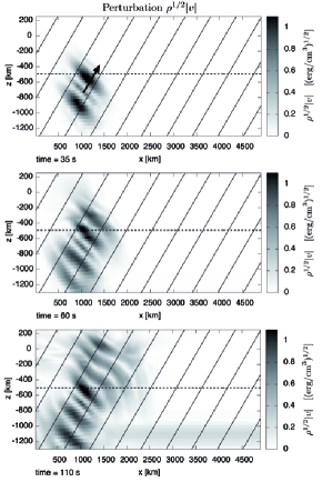
Figure 1: Velocity perturbation scaled with the density, $\rho^{1/2}|v|$, for different time steps. The magneto-acoustic wave propagates from the source (piston) located at $(x,z)=(1000~{}\mathrm{km},-750~{}\mathrm{km})$. The position of the piston and the direction of the excited wave front is indicated by the arrow in the top panel. The horizontal dashed line shows the equipartition layer, where the sound speed equals the Alfvén speed, $c_{\mathrm{s}}=c_{\mathrm{a}}$. The tilted vertical lines represent magnetic field lines.

The simulations are carried out using the CO⁵BOLD-code (Freytag, Steffen & Dorch, 2002; Schaffenberger et al., 2005, 2006), which solves the magnetohydrodynamic equations for a fully compressible gas including radiative transfer and a realistic equation of state.
The model atmosphere corresponds to the top part of Model S (Christensen-Dalsgaard et al., 1996) interpolated onto the grid of the simulation domain. Superimposed on the model atmosphere is a homogenous magnetic field with a field strength of 3000 G. In the first case of our investigations the magnetic field is tilted by an angle $\alpha=$ 30^∘ to the vertical axis. In the second case the orientation of the magnetic field with respect to the vertical axis is $\alpha=$ -30^∘. The atmosphere is then evolved for some time without applying any perturbations to settle to the quasi-hydrostatic state compatible with the present discretization.
The vertical extent of the simulation domain covers a range of 1700 km, of which 1300 km are below and 400 km are above optical depth unity. The horizontal extent of the atmosphere is 4900 km. In the vertical direction an adaptive grid with 58 cells is used. The grid resolution at the bottom of the simulation domain is 46 km while the resolution for the photosphere is 7 km. The horizontal direction is covered by 122 cells with a constant resolution of 40 km.
Transmitting boundary conditions are applied in the lateral and in the vertical direction. The magnetic field is kept constant at a specific angle to the vertical. This ensures that the magnetic field keeps its given orientation. Magneto-acoustic waves are excited using a piston, which is implemented as a small, gaussian shaped perturbation to the pressure gradient in the momentum equation. The center of the piston is placed at $(x,z)=(\mathrm{1000~{}km},-\mathrm{750~{}km})$ and the full width at half maximum of the gaussian is 200 km. The piston continuously launches sinusoidal waves with a monochromatic frequency of $f_{0}=20$ mHz. Although, lower frequencies would be more practical for actual detections in the solar case, the relatively high frequency was chosen for a good visualization of the mode transmission and conversion. Here, we are interested in propagating waves and not in frequencies near or below the cut-off frequency. One can expect a similar behavior of the wave propagation for all frequencies above the acoustic cut-off frequency, according to Khomenko & Collados (2006) and references therein, so that the 20 mHz waves should be a good representation for all waves above $\approx 5$ mHz.
The initial wave vector has an angle of 30^∘ to the vertical direction. Thus, for the first case the initial wave vector is parallel to the orientation of the magnetic field vector while in the second case the angle of incidence of the wave vector to the magnetic field vector (the “attack angle”) is about 60^∘. The piston is placed at a depth where plasma-$\beta\gg 1$. Thus, the excited waves are predominantly acoustic.
In the next section we will show how the magnetic field affects the propagation of magneto-acoustic waves.

3 Wave propagation in inclined magnetic fields

3.1 Small attack angle

First we consider the case where the magnetic field in the solar atmosphere is inclined by 30^∘ to the vertical direction. Thus, the movement of the piston is parallel to the magnetic field. This setup corresponds to the investigated case presented in the top panel of Fig. 3 in Cally (2007) except that we use a stronger magnetic field and high frequency waves.

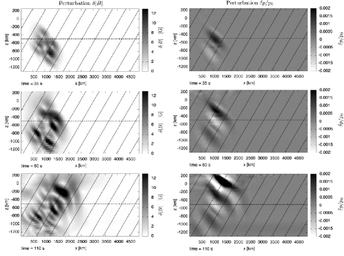
Figure 2: Left column: perturbation $\delta|B|$ of the magnetic field strength. Right column: pressure perturbation, $\delta p/p_{0}$, normalized to the local pressure. The horizontal line represents the equipartition layer and the tilted lines represent the magnetic field lines.

Fig. 1 shows the wave propagation of the magneto-acoustic wave for the velocity scaled with the density for different snapshots. In velocity, both magneto-acoustic waves, the slow and the fast mode, can be followed since both cause velocity perturbations. However, the different modes are not easily distinguishable. In order to follow the wave propagation of the slow mode only, which is predominantly an acoustic wave, the perturbation of the gas pressure is plotted in the right column of Fig. 2. As mentioned in Sect. 2, the wave is launched by the piston as a predominantly acoustic wave. Upon reaching the equipartition layer where the Alfvén speed reaches the sound speed, $c_{a}=c_{s}$, the acoustic wave is mostly transmitted, however it changes from the fast to the slow branch. The slow mode, which is predominantly an acoustic wave, is then guided along the field lines into the higher layers of the atmosphere as can be seen in the pressure perturbation. The evolution of the magnetic field perturbation is plotted in the left column of Fig. 2. Although the wave is launched parallel to the magnetic field vector, because of the gradient of the sound speed in the convection zone the wave vector is tilted gradually in more vertical direction as the wave travels towards the photosphere. Hence, at the equipartition layer the wave vector and magnetic field vector comprise a small angle, allowing only a small amount of the wave energy to be converted into a fast magneto-acoustic wave. This fast mode then gets turned around at the bottom of the photosphere because of the high gradient in Alfvén speed. However, most of the energy remains in the acoustic wave, which then reaches the higher layers of the atmosphere.

3.2 Large attack angle

In the second case, which we consider here, the magnetic field is inclined by -30^∘ to the vertical direction. The wave vector of the incident wave however stays the same as in the first case. Thus, the wave field comprises a large attack angle with the magnetic field. This case corresponds to the bottom panel of Fig. 3 in Cally (2007). Fig. 3 shows the perturbation of the pressure and the perturbation of the magnetic field.

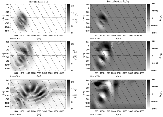
Figure 3: Left column: perturbation of the magnetic field strength, $\delta|B|$. Right column: perturbation of the pressure, $\delta p/p_{0}$, for different time steps. Note, that the plots in the last row can not be compared directly, since the plots show different snapshots (left plot at $t=185$ s; right plot at $t=100$ s). The last snapshot for $\delta|B|$ shows that the wave has undergone complete refraction and travels back to the solar interior.

At the equipartition layer the wave front again splits into two parts, whereby this time the fast magneto-acoustic wave receives more energy. The wave front that consists of the slow magneto-acoustic wave is again guided along the field lines into the higher solar atmosphere, as is visible from the pressure perturbation plotted in the right column of Fig. 3. The second and more dominant wave front is the fast magneto-acoustic wave emerging from the equipartition layer. Again, because of the high gradient of the Alfvén speed, the wave is refracted and turns around towards the solar interior.

3.3 Comparison of the acoustic flux for both cases

In order to demonstrate how mode conversion is affected by the attack angle, the vertical acoustic wave flux $F_{\mathrm{ac,z}}=\delta p*v_{z}$ is calculated. A comparison of the vertical acoustic flux for both cases, small and large attack angle, is plotted in Fig. 4 for the same time at $t=100$ s. When the angle between the wave vector and the magnetic field vector is small, most of the energy of the wave remains acoustic. The lower panel shows the case with the large attack angle. Only little acoustic energy is transmitted by the slow magneto-acoustic wave, visible in the upper left hand corner of the lower plot. The refracted acoustic flux is due to the nature of the magneto-acoustic wave, which causes non-vanishing gas pressure perturbations for both the fast and the slow modes. The fast mode however, is primarily dominated by the magnetic pressure. The acoustic flux is less than for the case where incident waves propagate parallel to the magnetic field.
Thus, most of the acoustic flux is transmitted when the wave vector and magnetic field vector are parallel at the equipartition layer. A large attack angle causes a major fraction of the wave energy to convert from acoustic to magnetic. Hence, it is not transported into the higher layers of the solar atmosphere because of the refraction of the fast mode.

4 Conclusions

Our results compare favorably with the wave propagation path and mode conversion as derived from ray conversion theory (Schunker and Cally, 2006; Cally, 2007) using a numerical code, which solves the magnetohydrodynamic equations for an ideal, compressible medium without any special precautions for the treatment of mode conversion. This gives us some confidence to apply the present code to more complex atmospheric configurations. In particular, the present method can be used to track waves into a dynamically evolving, convectively unstable atmosphere.
The amount of acoustic energy that is transmitted into the solar atmosphere depends strongly on the angle between the local wave vector and the magnetic field vector at the equipartition layer. Thus, this specific layer in the atmosphere acts as a filter where the slow and fast magneto-acoustic waves are separated and only the acoustic flux of the slow magneto-acoustic wave reaches the higher layers of the atmosphere.

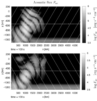
Figure 4: Vertical acoustic flux, $F_{\mathrm{ac,z}}$, for both test cases. Top: acoustic flux for the atmosphere with the wave vector almost parallel to the magnetic field. Bottom: acoustic flux for the case of the large attack angle.

Schunker and Cally (2006) and Cally (2007) also test the wave propagation for vertical magnetic fields. Due to the limited space, we omit these results here, but note that their and our results qualitatively agree.