YITP-10-84, IHES/P/10/34

Seiberg-Witten curve via generalized matrix model

Kazunobu Maruyoshi¹ and Futoshi Yagi²

¹Yukawa Institute for Theoretical Physics, Kyoto University, Kyoto 606-8502, Japan
²Institut des Hautes $\acute{E}$tudes Scientifiques, 91440, Bures-sur-Yvette, France

Abstract

We study the generalized matrix model which corresponds to the $n$-point toric Virasoro conformal block. This describes four-dimensional ${\mathcal{N}}=2$ $SU(2)^{n}$ gauge theory with circular quiver diagram by the AGT relation. We first verify that the generalized matrix model is obtained from the perturbative calculation of the Liouville correlation function. We then derive the Seiberg-Witten curve for ${\mathcal{N}}=2$ gauge theory as a spectral curve of the generalized matrix model.

1 Introduction

Recently, an interesting conjecture has been proposed in [1] that there are two equivalent ways for describing two M5-branes wrapped on a Riemann surface. One of the ways is a four-dimensional ${\mathcal{N}}=2$ superconformal $SU(2)$ quiver gauge theory, which is constructed depending on the number of genus and punctures of the Riemann surface [2, 3]. The other is the Liouville theory defined on that Riemann surface. The proposal, which is often called AGT conjecture [1], is that the Nekrasov partition function [4] of such quiver gauge theory can be reproduced by the $n$-point conformal block of the Virasoro algebra, where $n$ is the number of punctures. This conjecture has been generalized to the higher rank gauge group [5, 6, 7, 8], non-conformal case [9, 10, 11], and to the case in the presence with the surface and loop operators [12]–[24]. ( See also [25, 26] for the M-theory considerations.) A proof has been given in [27] and [28] for $SU(2)$ gauge theory with adjoint and ($N_{f}=0,1,2$) fundamental hypermultiplets by using the recursion relation [29, 30, 31, 32].

It was discussed in [33] that the AGT conjecture for the case on a sphere can be understood through a matrix model. The matrix model expression of the conformal block on a sphere is given by reinterpreting the Dotsenko-Fateev integral representation of it as the (beta-deformed) matrix integral [34, 35] with a logarithmic potential. When the central charge $c=1+6Q^{2}$ ($Q=b+1/b$) equals one, or equivalently, $b=i$, the conformal block is represented by the usual matrix model. The matrix model technique, in particular large $N$ limit, is useful to show that the gauge theory result can be reproduced [36, 37, 38, 39]. (See also [40] for $1/N$ correction.) It has been discussed that direct integral calculation leads to the instanton ($q$-)expansion of the Nekrasov partition function (and the corresponding expansion of the conformal block) [41, 42, 43, 44, 45, 46, 47].

While the understanding of the AGT conjecture for a sphere through the matrix model has been developed, a counterpart for a Riemann surface with higher genus is not yet fully understood. In this paper, we study the following integral:

$$Z=\int\prod_{i=1}^{N}dz_{i}\prod_{i<j}\theta_{*}(z_{i}-z_{j})^{-2b^{2}}\exp\left(-\frac{b}{g_{s}}\sum_{j=1}^{N}\left(\sum_{k=1}^{n}2m_{k}\log\theta_{*}(z_{j}-w_{k})+4\pi iaz_{j}\right)\right),$$ (1.1)

where the function $\theta_{*}(z)$ is defined in terms of the Jacobi theta function $\theta_{1}(z|\tau)$ and the Dedekind eta function $\eta(\tau)$ as $\theta_{*}(z)\equiv q^{-1/12}\theta_{1}(z|\tau)/\eta(\tau)$ with the fixed modulus $q=e^{2\pi i\tau}$ of the torus. This integral is an extension of the beta-deformed matrix model corresponding to the conformal block on the sphere to that on the torus with $n$ punctures, where $z-w$ is replaced by $\theta_{*}(z-w)$ [33]. A closely related free field representation for toric conformal block is discussed in [48].

Although this integral cannot be written in terms of a usual matrix integral, it can be seen as a “generalized matrix model”, whose “eigenvalues” $z_{i}$ live on the torus. Rigorously speaking, the integral is defined on the cover of the torus because the integrand itself is not completely doubly periodic. However, the positions of cuts, at which the eigenvalues are placed, are indeed doubly periodic. When we regard the integral variables $z_{i}$ as the eigenvalues, the product of theta functions $\prod_{i<j}\theta_{*}(z_{i}-z_{j})^{-2b^{2}}$ can be regarded as a counterpart of the Vandermonde determinant. This form is expected from the propagator of the two-dimensional free theory on a torus. The parameters $m_{k}$ are the momenta of the vertex operators while $w_{k}$ are their insertion points. The parameter $a$ and the filling fractions are identified as the internal momenta in the conformal block. The parameters in the integral are related as

$$\sum_{k=1}^{n}m_{k}+bg_{s}N=0$$ (1.2)

due to the momentum conservation law.

The AGT conjecture indicates that the $n$-point conformal block on a torus is related to the ${\mathcal{N}}=2$ superconformal $SU(2)^{n}$ gauge theory with a circular quiver diagram. The parameters $m_{k}$ are identified with the masses of the bifundamental hypermultiplets and the internal momenta of the conformal block correspond to the Coulomb moduli parameters. We see that such relation can be partially understood through the integral (1.1) in the large $N$ limit: On one hand, we show that the integral is derived from the perturbative calculation of the correlation function of the Liouville theory. On the other hand, we confirm that the spectral curve of the integral can be identified with the Seiberg-Witten curve of the quiver gauge theory.

The organization of this paper is as follows. In section 2, we review the M-theory construction of the four-dimensional superconformal $SU(2)^{n}$ gauge theory and see the M-theory curve which describes the low energy effective theory of the gauge theory. In section 3, we see that the integral representation (1.1) is derived from the Liouville $n$-point correlation function on a torus by perturbative calculation. We then discuss that the proposed integral (1.1) corresponds to the toric conformal block. In section 4, we consider the large $N$ spectral curve of the integral and identify it with the curve obtained in section 2. We conclude with discussions in section 5.

2 M-theory curve of $SU(2)$ quiver gauge theory

In this paper, we consider ${\mathcal{N}}=2$ superconformal $SU(2)^{n}$ gauge theory with circular quiver. This type of quiver gauge theory can be constructed as a worldvolume theory of D4-branes suspended between NS5-branes in type IIA string theory [2], as depicted in figure 1. The D4-branes occupy the $x^{0,1,2,3}$ and $x^{6}$ directions and the NS5-branes occupy $x^{0,1,2,3}$ and $x^{4,5}$. The $x^{4,5}$ coordinates are combined into the complex one $v=x^{4}+ix^{5}$. The difference of the $v$-coordinates of D4-branes in neighboring intervals of the NS5-branes is identified with the mass parameter of the bifundamental hypermultiplet. The $x^{6}$ direction is compactified and is periodic.

Figure 1: Brane configuration of the $SU(2)^{4}$ gauge theory with circular quiver. The D4-branes are suspended between the NS5-branes.

The curve which describes the low energy effective theory of this quiver gauge theory can be obtained by the M-theory up-lift by adding periodic $x^{10}$ direction and considering the hypersurface in $v,z=x^{6}+ix^{10}$ space. Since both the $x^{6}$ and $x^{10}$ directions are compactified, these represent a torus $E$. We denote this torus by Weierstrass form

$$y^{2}=4x^{3}-g_{2}x-g_{3},$$ (2.1)

where these coordinates are related to $z$ in terms of Weierstrass elliptic function as $x=\wp(z)$ and $y=\wp^{\prime}(z)$. The curve in $X=\mathbb{C}\times E$ which the M5-brane wraps on is identified with the Seiberg-Witten curve. For the $SU(2)^{n}$ case, the form of it is $F(x,y,v)=0$ with

$$F(x,y,v)=v^{2}-f_{1}(x,y)v+f_{2}(x,y).$$ (2.2)

The positions of $n$ NS5-branes are translated in M-theory to the points in the torus $E$ in which $f_{1}$ and $f_{2}$ have simple poles [2]. The residues of $f_{1}$ are interpreted as the mass parameters $m_{k}$ of the bifundamentals. (When we discuss poles or residues, we use the local coordinate $z=x^{6}+ix^{10}$.)

Note that the above consideration corresponds to the case where the total sum of the hypermultiplet masses vanishes:

$$\sum_{k=1}^{n}m_{k}=0.$$ (2.3)

In order to include the most generic case with non-zero sum $m$ of the masses, we have to consider non-trivial bundle $X_{m}\rightarrow E$ such that $x^{6}\rightarrow x^{6}+2\pi R$, $v\rightarrow v+m$, rather than the trivial bundle $X$. By this choice, the constraints on $f_{1}$ and $f_{2}$ are as follows: let $p_{k}\in E$ ($k=1,\ldots,n$) be the positions of the singularities coming from the NS5-branes. Then, $f_{1}$ and $f_{2}$ have order $1$ and $2$ poles respectively at, say $p_{1}$, and have simple poles at $p_{2},\ldots,p_{n}$. (Note that the sum of the residues of $f_{1}$ should vanish and therefore the residue at $p_{1}$ of $f_{1}$ is $-\sum_{k=2}^{n}m_{k}$.) Furthermore, the double pole of $f_{2}$ at $z_{1}$ disappears when we use a good coordinate $\tilde{v}=v+\frac{m}{4}\frac{y}{x}$.

However, as pointed out in [3], the problem can be simplified by eliminating the linear term in $v$ and writing the curve as follows

$$v^{2}=\phi_{2},$$ (2.4)

where we have shifted as $v\rightarrow v+\frac{f_{1}}{2}$ and therefore $\phi_{2}=\frac{f_{1}^{2}}{4}-f_{2}$. It follows from the above constraints that $\phi_{2}$ has double poles at $p_{1},p_{2},\ldots,p_{n}$ and the coefficients are simply the mass parameters $m_{k}^{2}$. The Coulomb branch parameters are included in less singular terms: we can introduce $n-1$ parameters $c_{k}$ by adding the functions which have simple poles at $p_{k}$ because the sum of the $c_{k}$ should vanish. We are also free to add the constant term in $\phi_{2}$. These correspond to $n$ Coulomb moduli parameters. Indeed, the most singular part of $\phi_{2}$ can be represented by $\wp(z)$ and the less singular part is by elliptic $\zeta$ function: $\wp=-\frac{d}{dz}\zeta$. Therefore, the curve is $v^{2}=\phi_{2}$ with

$$\phi_{2}=\sum_{k=1}^{n}m_{k}^{2}\wp(z-z_{k})+\sum_{k=1}^{n}c_{k}\zeta(z-z_{k})+A,$$ (2.5)

where $z_{k}$ are the values of the local coordinate $z=x^{6}+ix^{10}$ at the points $p_{k}$. This curve can be seen as a double cover of the torus with $n$ punctures whose positions are $z=z_{k}$. The Seiberg-Witten one form is represented by $vdz$.

3 From Liouville theory to generalized matrix model

In [1], it has been proposed that the $n$-point conformal block on a torus can be identified with the Nekrasov partition function of ${\mathcal{N}}=2$ quiver gauge theory discussed in the previous section. This relation for a torus was further studied in [51, 27]. The identification of the parameters of the two is as follows: the momenta of the vertex operators, the internal momenta and the complex structure moduli correspond, respectively, to the mass parameters of the hypermultiplets, the Coulomb moduli and the gauge coupling constants in the gauge theory. The Liouville correlation function can be obtained by integrating the contribution from the three-point function and the conformal block over the internal momenta. In this section, we explain how the integral representation (1.1) appears from the full correlation function, based on the discussion of [52, 33].

The $n$-point function of the Liouville theory on a torus is formally given by the following path integral

$$A\equiv\left<\prod_{k=1}^{n}e^{2m_{k}\phi(w_{k},\bar{w}_{k})}\right>_{{\rm Liouville\,\,on}\,\,T^{2}}=\int{\mathcal{D}}\phi(z,\bar{z})e^{-S[\phi]}\prod_{k=1}^{n}e^{2m_{k}\phi(w_{k},\bar{w}_{k})},$$ (3.1)

where the Liouville action is given by

$$S[\phi]=\int d^{2}z\sqrt{-g}\left(\frac{1}{4\pi}\partial_{a}\phi\partial^{a}\phi+\mu e^{2b\phi}\right),$$ (3.2)

under the flat background metric. We choose the insertion points $w_{k}$ such that they satisfy

$$\sum_{k=1}^{n}m_{k}w_{k}=0,$$ (3.3)

which does not break generality due to the translational invariance of the torus.

We divide the Liouville field into the zero mode and the fluctuation $\phi(z,\bar{z})=\phi_{0}+\tilde{\phi}(z,\bar{z})$. By integrating over $\phi_{0}$, we obtain

$$A = \frac{\mu^{-\sum_{k=1}^{n}\frac{m_{k}}{b}}}{2b}\Gamma\left(\sum_{k=1}^{n}\frac{m_{k}}{b}\right)\int{\mathcal{D}}\tilde{\phi}(z,\bar{z})e^{-S_{0}[\tilde{\phi}]}\left(\int d^{2}z\,\,e^{2b\tilde{\phi}(z,\bar{z})}\right)^{-\sum_{k}\frac{m_{k}}{b}}\prod_{k=1}^{n}e^{2m_{k}\tilde{\phi}(w_{k},\bar{w_{k}})},$$ (3.4)

where $S_{0}$ is the free scalar field action. When

$$N\equiv-\sum_{k=1}^{n}\frac{m_{k}}{b}\in\mathbb{Z}_{\geq 0},$$ (3.5)

the correlator diverges due to the factor $\Gamma(-N)$. Up to this divergent factor, the $n$-point correlation function $A$ is given by a perturbation from the free theory

$$A = \frac{\mu^{N}}{2b}\Gamma\left(-N\right)\int_{T^{2}}\prod_{i=1}^{N}d^{2}z_{i}\left\langle\prod_{i=1}^{N}:e^{2b\phi(z_{i},\bar{z}_{i})}:\,\,\prod_{k=1}^{n}:e^{2m_{k}\phi(w_{k},\bar{w}_{k})}:\right\rangle_{{\rm free\,\,on}\,\,T^{2}}.$$ (3.6)

The condition (3.5) ensures the momentum conservation in the free theory.

The $\ell$-point function of the free theory on a torus is given by

$$\left\langle\prod_{i=1}^{\ell}:e^{ik_{i}\phi(z_{i},\bar{z}_{i})}:\right\rangle_{{\rm free\,\,on}\,\,T^{2}}=iC_{T^{2}}^{X}(\tau)(2\pi)\delta(\sum_{i}k_{i})\prod_{i<j}\left|\eta(\tau)^{-3}\theta_{1}\left(z_{ij}|\tau\right)\exp\left[-\frac{\pi({\rm Im}z_{ij})^{2}}{\tau_{2}}\right]\right|^{k_{i}k_{j}},$$

(3.7)

where $z_{ij}\equiv z_{i}-z_{j}$, $\tau$ is the modulus of the torus, $\tau_{2}$ is its imaginary part, and $C_{T^{2}}^{X}=(4\pi^{2}\tau_{2})^{-\frac{1}{2}}|\eta(\tau)|^{-2}$. It factorizes into holomorphic and anti-holomorphic parts by introducing an additional integral as [54, 55, 53]

$$\left\langle\prod_{i=1}^{\ell}:e^{ik_{i}\phi(z_{i},\bar{z}_{i})}:\right\rangle_{{\rm free\,\,on}\,\,T^{2}}$$ (3.8)

$$=2i|\eta(\tau)|^{-2}\delta(\sum_{i}k_{i})\int^{\infty}_{-\infty}da\left|\left(\prod_{i<j}\left(\frac{\theta_{1}\left(z_{ij}|\tau\right)}{\eta(\tau)^{3}}\right)^{\frac{k_{i}k_{j}}{2}}\right)q^{a^{2}}\exp\left(-2\pi i\sum_{j=1}^{\ell}k_{j}z_{j}a\right)\right|^{2},$$ (3.9)

where $q=\exp(2\pi i\tau)$. We recover (3.7) by explicitly carrying out the Gaussian integral over $a$. This expression is more suitable for associating the Liouville $n$-point function to the holomorphic generalized matrix model.

Here, we introduce

$$\theta_{*}(z)\equiv q^{-1/12}\frac{\theta_{1}(z|\tau)}{\eta(\tau)}=2\sin(\pi z)\prod_{m=1}^{\infty}(1-e^{2\pi iz}q^{m})(1-e^{-2\pi iz}q^{m})$$ (3.10)

where $q=\exp(2\pi i\tau)$ is fixed, for later convenience. Using the explicit expression (3.9) for (3.6), we find that the $n$-point function $A$ of the Liouville theory reduces to the following integral

$$A = C(\tau,m_{k},b)\prod_{1\leq k<l\leq n}\left|\theta_{*}(w_{kl})\right|^{-4m_{k}m_{l}}\int^{i\infty}_{-i\infty}da\,\,|q|^{-2a^{2}}\int_{T^{2}}\prod_{i=1}^{N}d^{2}z_{i}$$ (3.12)

$$\qquad\left|\exp\left[-2b\sum_{i=1}^{N}\sum_{k=1}^{n}m_{k}\log\theta_{*}\left(z_{i}-w_{k}\right)-2b^{2}\sum_{1\leq i<j\leq N}\log\theta_{*}(z_{ij})-4\pi iba\sum_{i=1}^{N}z_{i}\right]\right|^{2},$$

where $w_{ij}\equiv w_{i}-w_{j}$, and we have introduced the factor in front of the $z$ integral as

$$C(\tau,m_{k},b)\equiv\frac{\mu^{N}\Gamma(-N)}{b}\delta(0)|\eta(\tau)|^{-2}|q^{-1/24}\eta(\tau)|^{-4\sum_{k}m_{k}{}^{2}-4b^{2}N}.$$ (3.13)

The discussion above is valid even for finite $N$. However, it is not straightforward to factorize the integrals over the torus into holomorphic and anti-holomorphic integrals for generic $N$. In order to proceed to the next step, we evaluate the integral (3.12) in the large $N$ limit. From the momentum conservation (3.5), we see that $m_{k}={\cal O}(N)$ as $b={\cal O}(1)$. Although the integral variable $a$ runs over the whole range of imaginary numbers, dependence on $a$ of the exponent appears when $a={\cal O}(N)$. We see that all the three terms in the exponent in (3.12) are all ${\cal O}(N^{2})$. In the large $N$ limit, the integral (3.12) is evaluated at the critical points of the exponent of the integrand. The conditions for the criticality of the exponent are given by

$$\sum_{k=1}^{n}m_{k}\frac{\theta_{*}^{\prime}(z_{i}-w_{k})}{\theta_{*}(z_{i}-w_{k})}+b\sum_{j\neq i}\frac{\theta_{*}^{\prime}(z_{ij})}{\theta_{*}(z_{ij})}+2\pi ia=0$$ (3.14)

where $\theta_{*}^{\prime}(z)\equiv\partial_{z}\theta_{*}(z)$. The conditions obtained from the $\bar{z}_{i}$-derivatives are just the complex conjugate of (3.14). It is remarkable that the conditions for criticality are separated into holomorphic and anti-holomorphic equations, which indicates that the integrals over the torus in (3.12) can be factorized into holomorphic and anti-holomorphic integrals in the large $N$ limit.

If we do not have the second term in (3.14), we have $n$ possible critical points for each variable $z_{i}$, assuming that the parameters $m_{k}$ are generic. We expect that the $n$ critical points are “diffused” to form line segments due to the second term, similarly to the case of the usual large $N$ matrix model. Then, the solutions of (3.14) are labelled by the filling fraction $\nu_{k}=bg_{s}N_{k}$, in which $N_{k}$ out of $N$ variables $z_{i}$ take the value on the $k$-th line segment. Here, we have introduced the parameter $g_{s}$, where $g_{s}N$ is finite in the large $N$ limit, for later convenience.

We define the contributions from the solution labelled by $\{\nu_{k}\}$ to the holomorphic integral as

$$Z(q,w_{k},m_{k},a,\nu_{k}) \equiv \int\prod_{i=1}^{N}dz_{i}\prod_{1\leq i<j\leq N}\theta_{*}(z_{ij})^{-2b^{2}}$$ (3.15)

$$~{}~{}~{}~{}~{}~{}\exp\left(-\frac{b}{g_{s}}\sum_{i=1}^{N}\left(\sum_{k=1}^{n}2m_{k}\log\theta_{*}(z_{i}-w_{k})+4\pi iaz_{i}\right)\right),$$

where we have rescaled the parameters as $m_{k}\rightarrow m_{k}/g_{s}$ and $a\rightarrow a/g_{s}$. The paths of the integrals are defined such that only the solution of (3.14) labelled by the fixed filling fractions $\{\nu_{k}\}$ contributes to the integrals. By regarding the factor $\prod_{1\leq i<j\leq N}\theta_{*}(z_{ij})^{-2b^{2}}$ as the generalization of the Vandermonde determinant, we see that the holomorphic integral (3.15) is “the generalized matrix model” with the action

$$W(z)=\sum_{k=1}^{n}2m_{k}\log\theta_{*}(z-w_{k})+4\pi iaz.$$ (3.16)

The integral in (3.12) is then obtained by integrating (3.15) and its complex conjugate over the filling fractions. Thus, in the large $N$ limit, the $n$-point function $A$ of the Liouville theory can be written as

$$A = \int^{i\infty}_{-i\infty}da\int d\nu_{1}\cdots d\nu_{n-1}$$ (3.17)

$$\left|\left(q^{-1/24}\eta(\tau)\right)^{-2\sum_{k}m_{k}{}^{2}/g_{s}^{2}}\left(\prod_{1\leq k<l\leq n}\theta_{*}(w_{kl})^{-2m_{k}m_{l}/g_{s}^{2}}\right)q^{-a^{2}/g_{s}^{2}}Z(q,w_{k},m_{k},a,\nu_{k})\right|^{2}\!\!\!\!,$$ (3.18)

where we have used that $C(\tau,m_{k},b)$ is approximated as $\left|q^{-1/24}\eta(\tau)\right|^{-4\sum_{k}m_{k}{}^{2}/g_{s}^{2}}$.

The total $n$ parameters, $a$ and the independent filling fractions $\nu_{1},\cdots,\nu_{n-1}$, can be identified with the $n$ internal momenta $\alpha_{1},\cdots,\alpha_{n}$ in the conformal block ${\mathcal{B}}(q,w_{k},m_{k},\alpha_{k})$ [33]. Under this identification, we see from (3.18) that $Z(q,w_{k},m_{k},a,\nu_{k})$ corresponds to the conformal block as well as the holomorphic contribution from the three-point functions.

In the next section, we relate the generalized matrix model (3.15) with the ${\mathcal{N}}=2$ quiver gauge theory in the previous section. Before going into it, let us see the remaining parts in (3.18) here. As discussed in [1], the gauge coupling constants $q_{i}=\exp(2\pi i\tau_{i})$ ($i=1,\cdots,n$) of the $SU(2)^{n}$ quiver gauge theory is related to the modulus $q=\exp(2\pi i\tau)$ of the torus and the insertion points $w_{i}$ of the $n$-point function of the Liouville theory as

$$q_{1}=e^{2\pi i(w_{1}-w_{2})},\quad q_{2}=e^{2\pi i(w_{2}-w_{3})},\quad\cdots,\quad q_{n-1}=e^{2\pi i(w_{n-1}-w_{n})},\quad q_{1}q_{2}\cdots q_{n}=q.$$ (3.19)

Using (3.10) and the definition for the Dedekind eta function $q^{-1/24}\eta(\tau)=\prod_{m=1}^{\infty}(1-q^{m}),$ the factor in front of $Z(q,w_{k},m_{k},a,\nu_{k})$ in (3.18) is rewritten in terms of $q_{i}$ as

$$\left(q^{-1/24}\eta(\tau)\right)^{-2\sum_{k}m_{k}{}^{2}/g_{s}^{2}}\prod_{1\leq k<l\leq n}\theta_{*}(w_{kl})^{-2m_{k}m_{l}/g_{s}^{2}}$$ (3.20)

$$=\prod_{k<l}\left((iq_{k}\cdots q_{l-1})^{m_{k}m_{l}/g_{s}^{2}}\right)\prod_{i=1}^{n}\prod_{k=0}^{\infty}\left(1-q_{i}q_{i+1}\cdots q_{i+k}\right)^{-2m_{i}m_{i+k+1}/g_{s}^{2}}$$ (3.21)

where the subscripts of $m_{i}$ and $q_{i}$ are considered modulo $n$. This factor has a close form as the $U(1)$ factor, which is explicitly written in [1]. Furthermore, the factor $q^{-a^{2}/g_{s}^{2}}$ in (3.18) corresponds to the tree level contribution to the prepotential.

In this section, we have derived the generalized matrix model from the Liouville correlation function by explicitly carrying out the perturbative calculation. In [33], it was discussed that the action (3.16) of the generalized matrix model is also expected from a geometrical argument in topological string theory in the context of the AGT conjecture.

4 Spectral curve of the generalized matrix model

In this section, we derive the spectral curve of the generalized matrix model, which is introduced in the previous section:

$$\exp\left(-\frac{1}{g_{s}^{2}}{\cal F}\right)=\int\prod_{i=1}^{N}d\lambda_{i}\exp\left(-\frac{b}{g_{s}}\sum_{i=1}^{N}W(\lambda_{i})+\sum_{i<j}\log\left(\theta_{*}(\lambda_{i}-\lambda_{j})\right)^{-2b^{2}}\right),$$ (4.1)

where $W(\lambda)$ is given by (3.16). As stated previously, the paths of the integrals are determined such that they realize the given filling fractions. For generic parameters, the action $W(\lambda)$ has $n$ critical points. In order to make the discussion as generic as possible, we will calculate it with a generic action with $n$ critical points and, at the final stage, substitute its specific form (3.16). We will see that the Seiberg-Witten curve (2.4) with (2.5) appears as the spectral curve of this generalized large $N$ matrix model.

In the large $N$ limit, the problem of the integration in (4.1) reduces to calculation of the critical point of its exponent. The prepotential is given by

$$-\frac{1}{g_{s}^{2}}{\cal F}=-\frac{b}{g_{s}}\sum_{i}W(\lambda_{i})-\sum_{i\neq j}b^{2}\log\theta_{*}(\lambda_{i}-\lambda_{j}),$$ (4.2)

where each eigenvalue satisfies the condition of criticality

$$0=\frac{1}{g_{s}}W^{\prime}(\lambda_{i})+2b\sum_{j(\neq i)}\frac{\theta_{*}^{\prime}(\lambda_{i}-\lambda_{j})}{\theta_{*}(\lambda_{i}-\lambda_{j})}.$$ (4.3)

It is natural to assume that the eigenvalues are distributed around the critical points of $W(\lambda)$ but in the form of line segment, similarly to the usual matrix model. We denote these line segments as $C_{k}$ where $k=1,\cdots n$. We do not assume that $C_{k}$ are on a real axis. However, we assume that $C_{k}$ do not include the singular points $w_{\ell}$, at which the action $W(\lambda)$ diverges. Suppose that $N_{k}$ eigenvalues are on the line segment $C_{k}$, where $N_{k}$ satisfies $\sum_{k=1}^{n}N_{k}=N$.

Here, we introduce the density of eigenvalues $\rho(\lambda)$ which has non-zero value only on the line segment $C_{k}$. Outside of these regions, we define that $\rho(\lambda)=0$. The density of eigenvalues is normalized as $\int_{C_{k}}d\lambda\rho(\lambda)=bg_{s}N_{k}\equiv\nu_{k}$. Using the variables introduced above, the prepotential and the condition for criticality are written as

$${\cal F}=\int_{\sum_{k}C_{k}}d\lambda\rho(\lambda)W(\lambda)+\int_{\sum_{k}C_{k}}d\lambda^{\prime}\int_{\sum_{k}C_{k}}d\lambda\rho(\lambda)\rho(\lambda^{\prime})\log\theta_{*}(\lambda-\lambda^{\prime}),$$ (4.4)

$$0=W(\lambda)^{\prime}+2\int_{\sum_{k}C_{k}}d\lambda^{\prime}\rho(\lambda^{\prime})\frac{\theta_{*}^{\prime}(\lambda-\lambda^{\prime})}{\theta_{*}(\lambda-\lambda^{\prime})},$$ (4.5)

respectively.

In order to solve this, we define the resolvent as

$$R(z)\equiv\int_{\sum_{k}C_{k}}d\lambda\,\rho(\lambda)\frac{\theta_{*}^{\prime}(z-\lambda)}{\theta_{*}(z-\lambda)}.$$ (4.6)

Since the behavior of the theta function around the zeros is $\theta_{*}(\varepsilon)\sim C\varepsilon+{\cal O}(\varepsilon^{3})$, $\theta_{*}^{\prime}(\varepsilon)\sim C+{\cal O}(\varepsilon^{2})$ for small $\varepsilon$, the structure of the singularity is similar to that of the usual matrix model if we focus on the fundamental region of the torus. The resolvent has cuts at the line segments $C_{k}$. Also, the filling fractions are obtained by integrating the resolvent along the cuts as

$$\nu_{k}=\frac{1}{2\pi i}\oint_{C_{k}}dzR(z).$$ (4.7)

The significant difference from the usual hermitian matrix model is that the resolvent has pseudo periodicity due to the theta function. Using the identity

$$\frac{d}{dz}\log\theta_{*}(z+m+n\tau,\tau)=-2\pi in+\frac{d}{dz}\log\theta_{*}(z,\tau),$$ (4.8)

which holds for arbitrary integer $m$ and $n$, the pseudo periodicity of the resolvent is shown to be given as

$$R(z+m+n\tau)=R(z)-2\pi inbg_{s}N.$$ (4.9)

We see that the resolvent is completely periodic for the $A$-cycle, which is parallel to the real axis, but some constant is added for the $B$-cycle. This pseudo periodicity gives great restriction on the possible form of the resolvent below.

On the line segments $C_{k}$, the resolvent is expected to behave as

$$R(z+i\varepsilon e^{i\varphi(z)})+R(z-i\varepsilon e^{i\varphi(z)})=2\int_{\sum_{k}C_{k}}d\lambda^{\prime}\rho(\lambda^{\prime})\frac{\theta_{*}^{\prime}(z-\lambda^{\prime})}{\theta_{*}(z-\lambda^{\prime})}=-W^{\prime}(z),$$ (4.10)

$$R(z+i\varepsilon e^{i\varphi(z)})-R(z-i\varepsilon e^{i\varphi(z)})=\oint_{z}d\lambda^{\prime}\rho(\lambda^{\prime})\frac{\theta_{*}^{\prime}(z-\lambda^{\prime})}{\theta_{*}(z-\lambda^{\prime})}=-2\pi i\rho(z),$$ (4.11)

where we take real number $\varepsilon$ infinitely small and $\varphi(z)$ is properly defined such that $z+i\varepsilon e^{i\varphi(z)}$ or $z-i\varepsilon e^{i\varphi(z)}$ does not go across the cuts $C_{k}$ when $z$ moves along $C_{k}$. The integral in (4.10) is principal integration, which is given as an average of integral along the path above the singularity and that below the singularity. The resolvent should be determined such that (4.10) and (4.11) are satisfied for $z\in C_{k}$, together with the periodicity (4.9).

A candidate of the solution for (4.10) is

$$R_{0}(z)=-\frac{1}{2}W^{\prime}(z).$$ (4.12)

However, it does not reproduce the correct structure of singularity expressed in (4.11). We need singular contributions:

$$R(z)=R_{0}(z)+R(z)_{\rm sing},$$ (4.13)

where (4.10) and (4.11) impose

$$R(z+i\varepsilon e^{i\varphi(z)})_{\rm sing}+R(z-i\varepsilon e^{i\varphi(z)})_{\rm sing} = 0.$$ (4.14)

$$R(z+i\varepsilon e^{i\varphi(z)})_{\rm sing}-R(z-i\varepsilon e^{i\varphi(z)})_{\rm sing} = -2\pi i\rho(z).$$ (4.15)

The above discussion is valid for generic action $W(z)$. In the following, we use the concrete form (3.16) to determine the resolvent $R(z)$. Since $R_{0}(z)$ is given by

$$R_{0}(z)=-\sum_{k=1}^{n}m_{k}\frac{d}{dz}\log\theta_{*}(z-w_{k})-2\pi ia,$$ (4.16)

we see that its pseudo periodicity is given by

$$R_{0}(z+m+n\tau)=R_{0}(z)-2\pi inbg_{s}N,$$ (4.17)

where we used the identity (4.8) and the momentum conservation (3.5). (Note that the parameters $m_{k}$ and $a$ have been rescaled.) Remarkably, the pseudo periodicity (4.17) for $R_{0}(z)$ exactly agrees with that of the resolvent $R(z)$ in (4.9). Therefore, we find that $R(z)_{\rm sing}$ is exactly doubly periodic.

On one hand, we find that the resolvent $R(z)$ has no singularity except for the cuts in the regions $C_{k}$ from the definition (4.6). On the other hand, we see from the explicit form (4.16) that $R_{0}(z)$ has simple poles at $z=w_{k}+m+n\tau$ and their residues are $-m_{k}$. Therefore, $R(z)_{\rm sing}$ must have both the cuts in the regions $C_{k}$ and simple poles with residues $m_{k}$ at $z=w_{k}+m+n\tau$.

From (4.14), we see that the sign of $R(z)_{\rm sing}$ changes when crossing the cut. Thus, $R(z)_{\rm sing}^{2}$ has no such discontinuity and all the cuts disappear. Since $R(z)_{\rm sing}^{2}$ has double poles at $z=w_{k}+m+n\tau$, the Laurent expansion of $R(z)_{\rm sing}^{2}$ at $z=w_{k}$ has not only $(z-w_{k})^{-2}$ terms but also $(z-w_{k})^{-1}$ terms due to contact terms. We denote the coefficients of such terms as $c_{k}$. Such doubly periodic function is uniquely determined, up to adding a constant, as a linear combination of the Weierstrass $\zeta$ function, which has one simple pole in the fundamental region, and of the Weierstrass $\wp$ function, which has one double pole in the fundamental region. This uniqueness is followed from the Liouville theorem, which ensures that a function holomorphic on the whole complex plane is only the constant function. In other words, we cannot add non-trivial function to the doubly periodic function without changing its structure of singularity.

From the discussion above, we have derived that $R(z)_{\rm sing}{}^{2}$ must be of the form

$$\left(R(z)+\frac{1}{2}W^{\prime}(z)\right)^{2}=R(z)_{\rm sing}{}^{2}=\sum_{k=1}^{n}m_{k}^{2}\wp(z-w_{k})+\sum_{k=1}^{n}c_{k}\zeta(z-w_{k})-C.$$ (4.18)

where the coefficients $c_{k}$ satisfy the condition

$$\sum_{k=1}^{n}c_{k}=0$$ (4.19)

so that (4.18) is doubly periodic. This is the spectral curve of the generalized matrix model. This spectral curve (4.18) coincides with the form of the Seiberg-Witten curve (2.4) with (2.5).

4.1 One-point function

In the following, we concentrate on the case of one-point function and determine the constant in the spectral curve under the approximation that $|a|$ is large enough. The spectral curve (4.18) for $n=1$ reduces to

$$R(z)_{\rm sing}{}^{2}=m^{2}\wp(z)-C,$$ (4.20)

where we used the condition (4.19). From (4.15), the density of eigenvalue is written as

$$\rho(\lambda)=(\pm)\frac{1}{\pi i}\sqrt{m^{2}\wp(\lambda)-C},$$ (4.21)

where the sign should be determined so that $-i\rho(\lambda)d\lambda$ is positive real on the integral path $C_{1}$.

The equation of motion (4.5) for $n=1$ reduces to

$$m\frac{\theta_{*}^{\prime}(\lambda)}{\theta_{*}(\lambda)}+2\pi ia+\int_{C_{1}}d\lambda^{\prime}\rho(\lambda^{\prime})\frac{\theta_{*}^{\prime}(\lambda-\lambda^{\prime})}{\theta_{*}(\lambda-\lambda^{\prime})}=0.$$ (4.22)

Now, suppose that $ia\gg 1$. In order that the eigenvalues satisfy the equation of motion, at least either the first or the third term of (4.22) must be large enough to compensate the second term. The first term becomes large if an eigenvalue is placed close to the singularity $\lambda=0$. The third term becomes large if the distribution $\rho(\lambda^{\prime})$ takes large value around the pole $\lambda^{\prime}=\lambda$ of the integrand. Since $\rho(\lambda^{\prime})$ is constrained by the normalization condition

$$\int_{C_{1}}d\lambda^{\prime}\rho(\lambda^{\prime})=bg_{s}N,$$ (4.23)

$\rho(\lambda^{\prime})$ must take large value only around the region close to $\lambda^{\prime}=\lambda$ and rapidly decrease as it goes apart in this case. However, since $\rho(\lambda^{\prime})$ is given by (4.21), this occurs only if $\lambda$ is close to the singularity $\lambda=0$. Thus, in any case, every eigenvalue $\lambda$ must be distributed very close to the singularity $\lambda=0$. In other words, the cut $C_{1}$ of the resolvent is placed very close to the singularity $z=0$ and its length is very short.

When $\lambda\sim 0$, the eigenvalue density (4.21) can be approximated as

$$\rho\sim(\pm)\frac{m}{\pi i}\sqrt{\frac{1}{\lambda^{2}}-c^{2}},$$ (4.24)

where we put $C\equiv m^{2}c^{2}$ for future convenience. Therefore, in this approximation, the endpoints $a_{1}$, $b_{1}$ of the cut $C_{1}$ ($\rho(a_{1})=\rho(b_{1})=0$) are

$$a_{1},b_{1}\sim\pm\frac{1}{c}.$$ (4.25)

Also, the equation of motion (4.22) can be approximated as

$$\frac{m}{\lambda}+2\pi ia+\int_{C_{1}}d\lambda^{\prime}\frac{\rho(\lambda^{\prime})}{\lambda-\lambda^{\prime}}=0.$$ (4.26)

Since the solution of the classical equation of motion is given by

$$\lambda=\frac{im}{2\pi a},$$ (4.27)

it is expected that the cut $C_{1}$ is placed around this point. Taking account the symmetry, most natural possibility is that the endpoints $a_{1},b_{1}=\pm 1/c$ are on the real axis and the path $C_{1}$ goes beyond the origin as in figure 3.

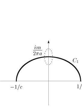
Figure 2: Path $C_{1}$

Figure 3: Path $C_{1}^{\prime}$

For later calculation, we analytically continue the eigenvalue density $\rho(\lambda)$, which has non-zero value only on the cut, to the whole complex plane and we denote it as $\tilde{\rho}(z)$. However, if we define $\tilde{\rho}(z)$ by the function in (4.24) under the usual convention that the function $f(z)=\sqrt{z}$ has cut on the negative real axis, it changes the sign across the imaginary axis. Since the original eigenvalue function $\rho(\lambda)$ does not have such discontinuity on $C_{1}$, we rewrite (4.24) and define $\tilde{\rho}(z)$ as

$$\tilde{\rho}(z)\equiv\frac{m}{\pi iz}\sqrt{1-(cz)^{2}},$$ (4.28)

so that it is smooth on the path $C_{1}$. The sign was determined so that $-i\tilde{\rho}(z)$ is positive at $z\sim im/a$.

At this stage, let us check the normalization condition (4.23). By using the analytically continued function (4.28), we can change the path of the integral from $C_{1}$ to $C_{1}^{\prime}$ as in figure 3 because there are no cuts or singularity between the path $C_{1}$ and $C_{1}^{\prime}$. Then, we can explicitly calculate the integral as

$$\int_{C_{1}}d\lambda\rho(\lambda) = \int_{-1/c}^{\varepsilon}dz\tilde{\rho}(z)+\int_{z=\varepsilon e^{i\theta},\theta:\pi\to 0}dz\tilde{\rho}(z)+\int_{\varepsilon}^{1/c}dz\tilde{\rho}(z)$$ (4.29)

$$= \int_{0}^{1/c}dz[\tilde{\rho}(z)+\tilde{\rho}(-z)]-\frac{1}{2}\times 2\pi i\,{\rm Res}_{z=0}\,\,\tilde{\rho}(z)$$ (4.30)

$$= -m.$$ (4.31)

Thus, taking account the momentum conservation $bg_{s}N+m=0,$ we find that the normalization (4.23) is satisfied for arbitrary $c$ and imposes no constraints.

We now use the equation of motion (4.26) at $\lambda=1/c$, which is the endpoint of the cut $C_{1}$.

$$cm+2\pi ia+\int_{C_{1}}d\lambda^{\prime}\frac{\rho(\lambda^{\prime})}{1/c-\lambda^{\prime}}=0.$$ (4.32)

By changing the path of the integral similarly to the previous calculation and by using (4.28), we find that the integral in the equations of motion can be explicitly calculated to give

$$\int_{C_{1}}d\lambda^{\prime}\frac{\rho(\lambda^{\prime})}{1/c-\lambda^{\prime}}=-(1+i)mc.$$ (4.33)

Thus, we have determined the coefficient $c$ as

$$c=\frac{2\pi a}{m},$$ (4.34)

which indicates $C=(2\pi a)^{2}$. Thus, the spectral curve (4.20) is

$$R(z)_{\rm sing}^{2}=m^{2}\wp(z)-(2\pi a)^{2}.$$ (4.35)

In the limit $|a|\gg|m|$, it is straightforward to check that

$$\int_{\beta}R(z)_{\rm sing}=2\pi im,~{}~{}~{}~{}~{}~{}\int_{\gamma}R(z)_{\rm sing}=2\pi ia,$$ (4.36)

where $\beta$ is the small cycle around the origin while $\gamma$ is the $A$-cycle of the torus. These are the expected property, which the Seiberg-Witten curve should satisfy. Thus, we have shown that the spectral curve of the generalized matrix model coincides with the Seiberg-Witten curve including the constant term in this limit.

5 Conclusion and discussion

In this paper, we have studied the generalized matrix model, which is a Dotsenko-Fateev type integral representation of the toric conformal block. This generalized matrix model is shown to be naturally derived from the perturbative calculation of the $n$-point function of the Liouville theory on the torus.

We have shown that the Seiberg-Witten curve of the corresponding gauge theory is derived from the generalized matrix model as a spectral curve. We have confirmed that the constants of the spectral curve of the generalized matrix model with $n=1$ agrees with those of the Seiberg-Witten curve for ${\mathcal{N}}=2^{*}$ theory in a large internal momentum limit. Our results suggest that the AGT relation between the Liouville theory on a torus and the four dimensional ${\cal N}=2$ quiver gauge theory can be understood through the generalized matrix model.

One of the future directions is to determine the undetermined constants in the spectral curve in more generically. Then, we go on to the next step to calculate the prepotential and compare the results with the conformal block or with the Nekrasov partition function.

Other direction is to consider a finite $N$ correction. We have seen the large $N$ limit has played an essential role to derive the generalized matrix model from the Liouville $n$-point function. Thus, such an extension seems to be quite non-trivial. In a sphere case, it is known that the matrix expression for the conformal block is valid even for finite $N$ [40] – [47]. So, it would be quite interesting to study whether such an expression is possible also for the torus case. In particular, the derivation of the loop equation would strongly help to calculate finite $N$ partition function [56, 57, 58].

The generalized matrix model which we have considered in this paper can be seen as an elliptic extension of the Selberg integral. The properties of this have been studied in [59, 60]. It would be interesting to study the generalized matrix model from this direction.

References

- [1] L. F. Alday, D. Gaiotto and Y. Tachikawa, “Liouville Correlation Functions from Four-dimensional Gauge Theories,” Lett. Math. Phys. 91, 167 (2010) [arXiv:0906.3219 [hep-th]].
- [2] E. Witten, “Solutions of four-dimensional field theories via M-theory,” Nucl. Phys. B 500, 3 (1997) [arXiv:hep-th/9703166].
- [3] D. Gaiotto, “N=2 dualities,” arXiv:0904.2715 [hep-th].
- [4] N. A. Nekrasov, “Seiberg-Witten Prepotential From Instanton Counting,” Adv. Theor. Math. Phys. 7, 831 (2004) [arXiv:hep-th/0206161].
- [5] N. Wyllard, “ conformal Toda field theory correlation functions from conformal N=2 SU(N) quiver gauge theories,” JHEP 0911, 002 (2009) [arXiv:0907.2189 [hep-th]].
- [6] A. Mironov and A. Morozov, “On AGT relation in the case of U(3),” Nucl. Phys. B 825, 1 (2010) [arXiv:0908.2569 [hep-th]].
- [7] S. Kanno, Y. Matsuo, S. Shiba and Y. Tachikawa, “N=2 gauge theories and degenerate fields of Toda theory,” Phys. Rev. D 81, 046004 (2010) [arXiv:0911.4787 [hep-th]].
- [8] S. Kanno, Y. Matsuo and S. Shiba, “Analysis of correlation functions in Toda theory and AGT-W relation for SU(3) quiver,” arXiv:1007.0601 [hep-th].
- [9] D. Gaiotto, “Asymptotically free N=2 theories and irregular conformal blocks,” arXiv:0908.0307 [hep-th].
- [10] A. Marshakov, A. Mironov and A. Morozov, “On non-conformal limit of the AGT relations,” Phys. Lett. B 682, 125 (2009) [arXiv:0909.2052 [hep-th]].
- [11] M. Taki, “On AGT Conjecture for Pure Super Yang-Mills and W-algebra,” arXiv:0912.4789 [hep-th].
- [12] L. F. Alday, D. Gaiotto, S. Gukov, Y. Tachikawa and H. Verlinde, “Loop and surface operators in N=2 gauge theory and Liouville modular geometry,” JHEP 1001, 113 (2010) [arXiv:0909.0945 [hep-th]].
- [13] N. Drukker, J. Gomis, T. Okuda and J. Teschner, “Gauge Theory Loop Operators and Liouville Theory,” JHEP 1002, 057 (2010) [arXiv:0909.1105 [hep-th]].
- [14] N. Drukker, D. Gaiotto and J. Gomis, “The Virtue of Defects in 4D Gauge Theories and 2D CFTs,” arXiv:1003.1112 [hep-th].
- [15] F. Passerini, “Gauge Theory Wilson Loops and Conformal Toda Field Theory,” JHEP 1003, 125 (2010) [arXiv:1003.1151 [hep-th]].
- [16] C. Kozcaz, S. Pasquetti and N. Wyllard, “A & B model approaches to surface operators and Toda theories,” JHEP 1008, 042 (2010) [arXiv:1004.2025 [hep-th]].
- [17] L. F. Alday and Y. Tachikawa, “Affine SL(2) conformal blocks from 4d gauge theories,” arXiv:1005.4469 [hep-th].
- [18] T. Dimofte, S. Gukov and L. Hollands, “Vortex Counting and Lagrangian 3-manifolds,” arXiv:1006.0977 [hep-th].
- [19] K. Maruyoshi and M. Taki, “Deformed Prepotential, Quantum Integrable System and Liouville Field Theory,” arXiv:1006.4505 [hep-th].
- [20] M. Taki, “Surface Operator, Bubbling Calabi-Yau and AGT Relation,” arXiv:1007.2524 [hep-th].
- [21] H. Awata, H. Fuji, H. Kanno, M. Manabe and Y. Yamada, “Localization with a Surface Operator, Irregular Conformal Blocks and Open Topological String,” arXiv:1008.0574 [hep-th].
- [22] C. Kozcaz, S. Pasquetti, F. Passerini and N. Wyllard, “Affine sl(N) conformal blocks from N=2 SU(N) gauge theories,” arXiv:1008.1412 [hep-th].
- [23] K. Hosomichi, S. Lee and J. Park, “AGT on the S-duality Wall,” arXiv:1009.0340 [hep-th].
- [24] T. S. Tai, “Uniformization, Calogero-Moser/Heun duality and Sutherland/bubbling pants,” arXiv:1008.4332 [hep-th].
- [25] G. Bonelli and A. Tanzini, “Hitchin systems, N=2 gauge theories and W-gravity,” Phys. Lett. B 691, 111 (2010) [arXiv:0909.4031 [hep-th]].
- [26] L. F. Alday, F. Benini and Y. Tachikawa, “Liouville/Toda central charges from M5-branes,” arXiv:0909.4776 [hep-th].
- [27] V. A. Fateev and A. V. Litvinov, “On AGT conjecture,” JHEP 1002, 014 (2010) [arXiv:0912.0504 [hep-th]].
- [28] L. Hadasz, Z. Jaskolski and P. Suchanek, “Proving the AGT relation for antifundamentals,” JHEP 1006, 046 (2010) [arXiv:1004.1841 [hep-th]].
- [29] A. B. Zamolodchikov, “Conformal Symmetry In Two-Dimensions: An Explicit Recurrence Formula For The Conformal Partial Wave Amplitude,” Commun. Math. Phys. 96, 419 (1984).
- [30] A. Marshakov, A. Mironov and A. Morozov, “Zamolodchikov asymptotic formula and instanton expansion in N=2 SUSY QCD,” JHEP 0911, 048 (2009) [arXiv:0909.3338 [hep-th]].
- [31] R. Poghossian, “Recursion relations in CFT and N=2 SYM theory,” JHEP 0912, 038 (2009) [arXiv:0909.3412 [hep-th]].
- [32] L. Hadasz, Z. Jaskolski and P. Suchanek, “Recursive representation of the torus 1-point conformal block,” arXiv:0911.2353 [hep-th].
- [33] R. Dijkgraaf and C. Vafa, “Toda Theories, Matrix Models, Topological Strings, and N=2 Gauge Systems,” arXiv:0909.2453 [hep-th].
- [34] V. S. Dotsenko and V. A. Fateev, “Conformal algebra and multipoint correlation functions in 2D statistical models,” Nucl. Phys. B 240, 312 (1984); V. S. Dotsenko and V. A. Fateev, “Four Point Correlation Functions And The Operator Algebra In The Two-Dimensional Conformal Invariant Theories With The Central Charge C1,” Nucl. Phys. B 251, 691 (1985).
- [35] A. Marshakov, A. Mironov and A. Morozov, “Generalized matrix models as conformal field theories: Discrete case,” Phys. Lett. B 265, 99 (1991); S. Kharchev, . A. Marshakov, A. Mironov, A. Morozov and S. Pakuliak, “Conformal Matrix Models As An Alternative To Conventional Multimatrix Models,” Nucl. Phys. B 404, 717 (1993) [arXiv:hep-th/9208044].
- [36] H. Itoyama, K. Maruyoshi and T. Oota, “The Quiver Matrix Model and 2d-4d Conformal Connection,” Prog. Theor. Phys. 123, 957 (2010) [arXiv:0911.4244 [hep-th]].
- [37] T. Eguchi and K. Maruyoshi, “Penner Type Matrix Model and Seiberg-Witten Theory,” JHEP 1002, 022 (2010) [arXiv:0911.4797 [hep-th]].
- [38] R. Schiappa and N. Wyllard, “An threesome: Matrix models, 2d CFTs and 4d N=2 gauge theories,” arXiv:0911.5337 [hep-th].
- [39] T. Eguchi and K. Maruyoshi, “Seiberg-Witten theory, matrix model and AGT relation,” arXiv:1006.0828 [hep-th].
- [40] M. Fujita, Y. Hatsuda and T. S. Tai, “Genus-one correction to asymptotically free Seiberg-Witten prepotential from Dijkgraaf-Vafa matrix model,” JHEP 1003, 046 (2010) [arXiv:0912.2988 [hep-th]].
- [41] A. Mironov, A. Morozov and S. Shakirov, “Matrix Model Conjecture for Exact BS Periods and Nekrasov Functions,” JHEP 1002, 030 (2010) [arXiv:0911.5721 [hep-th]].
- [42] A. Mironov, A. Morozov and S. Shakirov, “Conformal blocks as Dotsenko-Fateev Integral Discriminants,” Int. J. Mod. Phys. A 25, 3173 (2010) [arXiv:1001.0563 [hep-th]].
- [43] H. Itoyama and T. Oota, “Method of Generating q-Expansion Coefficients for Conformal Block and N=2 Nekrasov Function by beta-Deformed Matrix Model,” Nucl. Phys. B 838, 298 (2010) [arXiv:1003.2929 [hep-th]].
- [44] A. Mironov, A. Morozov and A. Morozov, “Matrix model version of AGT conjecture and generalized Selberg integrals,” arXiv:1003.5752 [hep-th].
- [45] A. Morozov and S. Shakirov, “The matrix model version of AGT conjecture and CIV-DV prepotential,” arXiv:1004.2917 [hep-th].
- [46] A. Morozov and S. Shakirov, “From Brezin-Hikami to Harer-Zagier formulas for Gaussian correlators,” arXiv:1007.4100 [hep-th].
- [47] H. Itoyama, T. Oota and N. Yonezawa, “Massive Scaling Limit of beta-Deformed Matrix Model of Selberg Type,” arXiv:1008.1861 [hep-th].
- [48] G. Felder, “BRST Approach to Minimal Methods,” Nucl. Phys. B 317, 215 (1989) [Erratum-ibid. B 324, 548 (1989)].
- [49] N. Seiberg and E. Witten, “Monopoles, duality and chiral symmetry breaking in N=2 supersymmetric QCD,” Nucl. Phys. B 431, 484 (1994) [arXiv:hep-th/9408099].
- [50] R. Donagi and E. Witten, “Supersymmetric Yang-Mills Theory And Integrable Systems,” Nucl. Phys. B 460, 299 (1996) [arXiv:hep-th/9510101].
- [51] V. Alba and A. Morozov, “Non-conformal limit of AGT relation from the 1-point torus conformal block,” arXiv:0911.0363 [hep-th].
- [52] M. Goulian and M. Li, “Correlation functions in Liouville theory,” Phys. Rev. Lett. 66 (1991) 2051.
- [53] E. D’Hoker and D. H. Phong, “The Geometry of String Perturbation Theory,” Rev. Mod. Phys. 60, 917 (1988).
- [54] E. P. Verlinde and H. L. Verlinde, “Multiloop Calculations in Covariant Superstring Theory,” Phys. Lett. B 192, 95 (1987).
- [55] R. Dijkgraaf, E. P. Verlinde and H. L. Verlinde, “C = 1 Conformal Field Theories on Riemann Surfaces,” Commun. Math. Phys. 115 (1988) 649.
- [56] J. Ambjorn, L. Chekhov, C. F. Kristjansen and Yu. Makeenko, “Matrix model calculations beyond the spherical limit,” Nucl. Phys. B 404, 127 (1993) [Erratum-ibid. B 449, 681 (1995)] [arXiv:hep-th/9302014].
- [57] G. Akemann, “Higher genus correlators for the Hermitian matrix model with multiple cuts,” Nucl. Phys. B 482, 403 (1996) [arXiv:hep-th/9606004].
- [58] B. Eynard and N. Orantin, “Invariants of algebraic curves and topological expansion,” arXiv:math-ph/0702045.
- [59] G. Felder, L. Stevens, and A. Varchenko, “Elliptic Selberg Integrals and Conformal Blocks,” arXiv:math/0210040 [math.QA].
- [60] V. P. Spiridonov, “Elliptic Hypergeometric Integrals,” arXiv:math/0303205 [math.CA].