A positive-weight next-to-leading order simulation of weak boson pair production.
Abstract:
In this article we describe simulations of , and production based on the positive weight next-to-leading-order (NLO) matching scheme, Powheg, in the Herwig++ event generator. Building on earlier efforts within the Herwig++ framework, the simulation includes a full description of truncated showering effects, required to correctly model soft, wide angle, emissions in angular-ordered parton showers. We utilize simple relations among each of the diboson cross sections, holding to , in constructing the simulation. Spin correlation effects are also included in the decays of the vector bosons at the tree order. A large part of this work is concerned with a full and thorough validation of the simulations through comparisons with alternative methods and calculations.
1 Introduction
The production of electroweak gauge boson pairs is a subject of significant interest in collider physics. Weak boson pair production was first studied in detail at LEP2, at centre-of-mass energies of up to [1, 2, 3, 4, 5], with the aim of precisely measuring the boson mass and with a view to directly probing and testing the non-Abelian character of the Standard Model gauge structure. In the period 1996-2000 approximately 40000 and 1000 events were recorded by the four LEP experiments [6]. At the Tevatron and production have also been the focus of extensive analysis by the CDF and D0 collaborations [7, 8, 9, 10, 11, 12, 13, 14, 15], albeit with an estimated factor of twenty less diboson events per experiment, based on their most recent publications. Recently the observation of production has also been reported by CDF and D0.
Although all of these LEP2 and Tevatron measurements are in agreement with Standard Model predictions, it is generally considered that should non-Standard Model physics play a role in this process, its effects will be manifest greater at greater energy scales. In particular, the effects of anomalous and triple gauge boson couplings, are predicted to grow with the invariant mass of the gauge boson pair [16]. Thus, even though fewer events will be recorded, the high energy data still being accumulated by CDF and D0 combined, has the potential to surpass the sensitivity of the LEP2 data to such effects. At the LHC the inclusive cross section for vector boson pair production is around a factor of ten higher than at the Tevatron, moreover, the luminosity is also substantially higher. It is then expected that in the near future very large quantities of high energy weak boson pairs will be recorded by the LHC experiments and that the non-Abelian nature of the weak bosons will be tested with a new level of vigor. To facilitate such precision tests theoretical predictions, ideally in the form of fully exclusive Monte Carlo simulations, should be made as accurate as possible.
Aside from being an interesting process in its own right, weak boson pair production deserves to be thoroughly understood given its role as an important background in many searches for currently undiscovered particles, most notably the Higgs boson. Notwithstanding the fact that the latest Tevatron analysis excludes, at the 95% confidence level, the Standard Model Higgs boson from having a mass in the range GeV [17], if the mass is above GeV the Higgs boson will primarily decay into or pairs [18, 19, 20, 21, 22]. Moreover, alternative models with extended Higgs sectors can yield large branching fractions for charged Higgs bosons decaying into pairs [23]. pair production is also a problematic background in studies of strong scattering [24] and in many supersymmetry search channels, specifically, those associated with a trilepton final state and missing transverse energy [25, 26, 27]. As with the dedicated studies of weak boson pair production discussed above, the discovery potential of these ongoing and imminent analyses depends heavily on the quality of the theoretical inputs.
In general, the main source of uncertainty associated with leading order theoretical predictions for hadronic collisions comes in the form of next-to-leading order QCD corrections. Next-to-leading order (NLO) QCD corrections to , and production were first calculated and studied in the early nineties by two separate groups [28, 29, 30, 31, 32, 33]. Some years later these results were improved upon by Dixon et al, who performed the calculations at the level of helicity amplitudes, thus providing full knowledge of the corrections to these processes including the leptonic decays of the massive vector bosons [34, 35]. Further improvements were made by Campbell and Ellis who extended the results of the latter work beyond the narrow width approximation, including contributions from singly resonant Feynman diagrams and interference effects between intermediate bosons and photons[36].
Following these results, in the early part of the last decade, a number of ground breaking developments took place in the field of Monte Carlo event generator research, most significantly, the invention of the CKKW(-L) and MLM algorithms, combining parton shower simulations together with those based on tree level matrix elements [37, 38, 39, 40, 41, 42] and, separately, the Mc@nlo [43] and Powheg [44, 45] formalisms for consistently including fully differential NLO corrections in parton shower simulations. In fact the Mc@nlo formalism was first successfully demonstrated through the simulation of pair production and the first public release of the program comprised of , and production, two years after the work of Campbell and Ellis. An impressive number of important Standard Model processes can now be simulated with the Mc@nlo program [46, 47, 48, 49], in addition, the modeling of unstable particle production has been enhanced through the inclusion of full spin correlations in the leading order and real contributions by the method developed in Ref. [50]. Nowadays a similar number of processes may also be simulated with publicly available programs based on the alternative Powheg formalism [51, 52, 53, 54, 55, 56, 57, 58, 59], first realized in the case of hadroproduction in 2006 [60].
Lately significant steps have been taken in the direction of automating the Mc@nlo and Powheg methods [61, 59, 62]. The most recent of these efforts features Powheg simulations of and production, integrating the calculation of Campbell and Ellis within the framework of the Sherpa event generator [62]. This simulation therefore includes singly resonant contributions, in particular interference effects in and pair hadroproduction, which are not included in the program discussed here. For reasons of technical simplicity, greatly increased computational efficiency, and minded to best utilize the existing Herwig++ infrastructure, e.g. the facility to include higher order QCD and QED corrections to the decays of vector bosons, we have based our work on the original calculations of Frixione et al. [28, 32, 33], as in Mc@nlo, valid in the double pole approximation.
We also note that many important collider physics analyses, such as the study of the di-vector boson signal [8, 11, 10, 63, 64, 65, 66, 67] and anomalous triple gauge boson couplings [10, 68, 69], employ invariant mass cuts on the vector boson decay products – almost always to bosons – which generally reduces the singly resonant contributions to negligible levels. The same is true of Higgs boson searches involving final-states comprising of bosons [70]. In the case of the boson the same invariant mass cuts around the boson decay products are not necessary since, in the case of the , the singly resonant contributions are only able to become sizable through interference. Thus, in pair production the singly resonant terms are subject to a simple Breit-Wigner suppression. Accordingly, the program presented here can be applied to the simulation of pair production for study as a signal process and as a background to Higgs boson production, as an alternative to the Mc@nlo program [13, 71, 72, 73]. Furthermore, as is usually the case in higher order calculations involving unstable particles, an ad hoc scheme is adopted in Ref. [36] to include the width of the vector bosons which, in this case, mistreats the singly resonant parts, particularly in the doubly resonant region. Nevertheless, it is incumbent upon us to point out that should analyses not include some form of cut on boson decay products, limiting, in particular, interference contributions, the matrix elements of Campbell and Ellis will continue to provide a good description of the production and decay processes, whereas those used here, like those of the underlying LO Herwig++ simulation, will fail. Analyses not employing such cuts are typical of general searches for physics beyond the Standard Model e.g. the search for SUSY in the trilepton channel, for which singly resonant contributions are expected to add around 15% to the doubly resonant background 111A study of the impact of singly resonant diagrams on such an analysis can be found in Ref. [36]..
In what follows we present an application of the Powheg method to Monte Carlo simulations of weak boson pair production within the Herwig++ event generator [74, 75], including a full validation. In Sect. 2 we briefly recall the basic Powheg algorithm and give details concerning how the NLO cross section is organized in a form amenable to its implementation; the section closes with a discussion of the associated NLO matrix elements [28, 32, 33], noting exact relations between the , , and next-to-leading order cross sections. In Section 3 we describe the key points in the simulation process, including the implementation of truncated and vetoed parton showers, occurring after the hardest emission has been generated. In Section 4 we show results from our implementation, comparing it to two independent NLO programs, Mcfm and Mc@nlo, before summarizing our findings in Sect. 5.
2 Hardest emission cross sections
The starting point for all Powheg simulations is the so-called hardest emission cross section, specifically, a matching between the constituents of the exact NLO differential cross section and the corresponding leading-log resummed cross section implicit in parton shower simulations [44]. For simple processes, such as the one we are considering, it can be written simply as
| (1) |
where are Born variables, which fully determine the kinematics of leading order configurations, and are radiative variables, parametrizing the kinematics of the hardest emission with respect to . and are the leading and next-to-leading order differential cross sections respectively, while is simply the bare, tree level, real emission cross section. The function may be expressed as
| (2) |
being the finite combination of, unresolvable, soft emission and virtual loop corrections, while corresponds to the remaining, regularized, real emission corrections. The Powheg Sudakov form factor for the hardest emission, , is defined as
| (3) |
where tends to the transverse momentum of the emitted parton in the soft and collinear limits. Emissions for which are considered as being unresolvable. In the ensuing subsections we give details concerning the components of the hardest emission cross section for the case of weak boson pair production (Eq. 1) , focusing on the function and its regularization.
2.1 Kinematics and phase space
In this subsection we begin by giving details regarding our parametrization of the kinematics for the hadroproduction of a pair of weak vector bosons, with and without the emission of an additional radiated parton. For both classes of event we denote the momenta of the partons incident from the directions by , while those of the weak bosons are labelled and . In discussing three-body, real emission, contributions the momentum of the additional, radiated, parton is denoted . Also, since we shall frequently refer to the sum of the weak boson momenta, we define .
The parametrization of our two- and three-body kinematics is taken to be identical to that in Refs. [28, 32, 33]. To this end we first define precisely what we mean by the rest frame of the vector boson pair. In the context of three-body events, for and collisions, we shall use this term to refer to the frame in which the vector bosons are balanced in their three-momenta, with the incoming quark defining the axis and the transverse momentum of the other initial-state parton defining the axis; for collisions the gluon replaces the quark in defining the axis. For genuine two-body events the latter criterion, concerning the definition of the axis, is omitted since for such events and are naturally acolinear.
We now introduce a set of Born variables and a set of radiative variables , clearly defined as follows:
-
- the invariant mass squared of the vector boson pair
-
- the rapidity of the weak boson pair in the lab frame
-
- the polar angle of in the rest frame of the vector boson pair
-
- the azimuthal angle of in the rest frame of the vector boson pair
-
- the ratio where, as usual,
-
- the cosine of the polar angle of momentum in the partonic
-
centre-of-mass frame
Both and range between and . Given a set of Born variables one can readily construct the momenta in the lab frame for two-body reactions, while augmenting these with a set of radiative variables enables one to fully reconstruct radiative processes in the lab frame. For the latter case explicit expressions for the momenta in the rest frame of the vector boson pair are given in Ref. [32]. Since these are unwieldy, yet straightforward, we do not reproduce them here. When reconstructing the three-body events using the aforesaid formulae, all particles are then returned to the lab frame by applying the following Lorentz transformation, , to each one:
| (4) |
The first component of this transformation, , is a rotation of angle in the plane, where is the transverse momentum of the vector boson system in the lab and partonic centre-of-mass frames:
| (5) |
Following a transverse Lorentz boost, , is carried out such that the momentum of the stationary vector boson system, , becomes , where we have defined . Lastly a longitudinal boost, , gives the vector boson system rapidity , returning all particles to the lab frame and completing the momentum reconstruction. Note that the ultimate step in the generation of all Powheg events involves randomizing the azimuthal orientation.
The final kinematic quantities we wish to declare are the momentum fractions of the incoming partons with respect to the beam particles. These are not independent degrees of freedom but functions of and, in the case of three-body final-states, . Taking to represent the momenta of the parent beam hadrons, the momentum fractions are defined according to the relation , whereupon it follows that
| (6) |
with being the hadronic centre-of-mass energy. Note that for genuine two-body final states, namely those corresponding to leading order and virtual contributions, the limit is clearly implied in the evaluation of the all kinematics quantities, including the momentum fractions i.e. for such final states .
Having described the parameterization of the kinematics we move to specify the integration measures in the two- and three-body phase spaces, for non-radiative and radiative events respectively. With these definitions in hand the phase space for the leading-order process can then be written as
| (7) |
where the two-body phase space measure for the vector boson system. In the centre-of-mass frame of , using conventional dimensional regularization, with dimensions
| (8) |
where is the magnitude of the three momentum of either weak boson in their rest frame.
To parametrize the three-body phase space we factorize it into a product of two two-body phase spaces for the reactions and , by inserting the identity in the form of an integral over a delta function defining as . In this way we may readily write the phase space measure as
| (9) |
where222An irrelevant overall factor has been dropped in writing since it is equal to .
| (10) |
and
| (11) |
The constant appears due to the use of dimensional regularization, it is given by
| (12) |
We emphasize that both and range between and , hence . It is also worth noting that and .
Since we restrict ourselves to processes for which the NLO corrections contain at most soft and initial-state collinear singularities, the product of with the squared real emission matrix elements will be finite throughout the radiative phase space. With this in mind, following Refs. [28, 76], we extract a factor of from and then expand it in powers of , to give
| (13) |
in which
| (14) | |||||
| (15) | |||||
| (16) |
where and , and being the masses of the weak vector bosons. The -distributions appearing in Eqs. 15 and 16 are defined according to the relation
| (17) |
for any sufficiently regular test function : in this case, the product of with the real emission matrix elements.
For completeness, we note that the kinematic boundaries are
| (18) |
with given by
| (19) |
In order to ease the numerical implementation of the distributions we map the variable into , defined according to
| (20) |
Whereas the integration domain was dependent on , the integral simply ranges from to .
2.2 Differential cross section
In this section we enumerate the various contributions to the NLO differential cross section. These are obtained by simply considering the product of the matrix elements with the phase space measures as written in Eq. 7 and Eqs. 9-17, exploiting simplifications arising in the soft and collinear limits to integrate out radiative variables. The discussion here is rather similar to that in our earlier work [56], including some minor changes and clarifications, indeed the formulae in that article were derived with the current application in mind, so we shall be brief.
In the following we shall refer to the parton types incident from the and directions as and respectively. We denote the parton distribution function (PDF) for a parton of type inside a beam hadron traveling in the direction by , where is the factorization scale. For brevity we then introduce the luminosity function, , as the product of the PDFs associated to and :
| (21) |
The leading order contribution to the differential cross section is given by the product of the leading order spin and colour averaged squared amplitude, , together with the luminosity function and flux factor:
| (22) |
In all cases, due to the universal nature of the infrared divergences in the one-loop amplitudes, the virtual corrections to can be generically written in the form
| (23) |
where the first term is universal and divergent, with given by
| (24) |
while the second is process dependent and finite as . For completeness, we define the bare virtual cross section and function by analogy to the corresponding leading order quantities:
| (25) |
The differential cross sections for the real emission processes, , take the following general form
| (26) |
For each flavour combination we consider these corrections to comprise of three components, corresponding to the three terms , and in the phase space Jacobian, Eqs. 14-16. We shall refer to these components as the soft, collinear, and hard / resolved contributions to the cross section.
The squared matrix elements for the real emission processes, in which a gluon is emitted from an initial-state quark or antiquark, factorize in the limit that the gluon is soft according to
| (27) |
Thus, for the integrand in Eq. 26 is entirely independent of the radiative phase space and it becomes trivial to integrate over . In doing this one finds the following expression for the soft contribution to the differential cross section:
| (28) |
All other sources of real corrections involve the emission of a quark or antiquark from external initial-state gluons, as such they do not contribute to the cross section in the soft limit; by contrast to the case of gluon emission, the matrix elements for such processes are regular in the limit , hence when they multiply the factor of in (Eq. 13) the result is zero.
We shall now turn our attention to the collinear limits. Since the real emission corrections to the process we are considering do not involve internal gluon lines, in the limit the spin averaged squared matrix elements factorize trivially according to333In Eqs. 27 and 29 we show only the leading term in since all others ultimately vanish due to the factor of in Eq. 13.
| (29) |
where or for respectively and denotes the type of the emitted parton. Considering only those terms in the phase space Jacobian proportional to we then obtain the following expression for the collinear contribution to the cross section
| (30) | |||||
where in the case that parton splits to produce parton , and for the case that parton branches to produce . The functions are the bare Altarelli-Parisi splitting kernels in dimensions, explicit expressions for which can be found throughout the literature e.g. Refs. [77, 56], while denotes their regularized counterparts (Appendix A); the soft-collinear cross section, , is entirely due to the term present in the latter. Lastly we declare to be the ratio of the luminosity function evaluated at with respect to that found in the leading order cross section viz
| (31) |
The singular parts of the collinear contribution proportional to the regularized Altarelli-Parisi functions, , are exactly canceled by collinear counterterms in the scheme, thus they play no further role in our discussion.
Finally, considering the third part of the phase space Jacobian, we have that the hard / resolved contribution to the real emission cross section is given by
| (32) | |||||
| (33) |
Combining all of the various pieces together we are able to write the next-to-leading order differential cross section as
| (34) |
where the second term is given by the finite sum of the bare virtual corrections, , the soft real emission contributions, , and the soft-collinear contributions, . The function is comprised of the remaining collinear and hard / resolved real emission corrections,
| (35) | |||||
Although it is not explicitly stated above, a summation over all contributing channels and flavour combinations is implied. Furthermore, in the case of the and initiated real emission corrections, one of the terms proportional to in the function should be omitted, either if is a gluon, or if is a gluon, since collinear branchings of the initial-state quarks do not occur in those processes.
2.3 Matrix elements
As noted in the introduction the simulation described in this article uses the NLO QCD calculations for , and production of Frixione et al. [28, 32, 33]. We have observed that these computations share a common underlying structure which we have exploited here. In particular we find that all production matrix elements, leading-order, real and virtual, are simply related to the corresponding production matrix elements by the following replacements:
| (36) |
where the quantities on the left are written using the notation of the production publication [32] and those on the right use that of the article [28]. In the latter work and denote the left handed couplings of the boson to up- and down-type quarks, is the boson coupling to quark flavours and , while is the trilinear gauge coupling . In Ref. [28] and are the vector and axial-vector couplings of the bosons to the colliding quarks.
We also find that the matrix elements are simply related to those of production by
| (37) |
where on the left denotes the relevant Cabibbo-Kobayashi-Maskawa matrix element in production, while on the right is used to refer to the flavour of the colliding quarks (up- or down-type). The functions and are the coefficients of those parts of the matrix elements corresponding to s-channel trilinear gauge-boson graphs interfering with themselves and with t-channel graphs respectively.
The validity of these relations was examined analytically using Mathematica444A Mathematica file detailing these checks for all cross section formulae in Refs. [28, 32, 33] is available from the author on request. These checks also reveal that, in both cases, all matrix elements satisfy additional symmetries involving the momenta of the final state vector bosons before the last transformation, / , is carried out; further exploration of this point is beyond the scope of this work.. In our simulation we have employed the matrix elements of Ref. [32] for production and applied the transformations in Eqs. 36 and 37 to these when generating and production events respectively. The correctness of relations Eqs. 36 and 37 at NLO is tested again, numerically, by comparing to alternative calculations in Mcfm and Mc@nlo.
We attribute the fact that these relations hold at the NLO level to the deceptively simple Dirac structure in the real and virtual corrections. In the beginnings of Refs. [28, 32, 33] it is observed that, for both sets of radiative corrections, all of the Dirac traces can be expressed in the form , where and are constants and is an arbitrary string of matrices, excluding . In the case of the virtual corrections the term never contributes to the final trace: it leads to a term proportional to the antisymmetric Levi-Civita tensor, for which there are not enough linearly independent momenta available to give rise to a non-vanishing contribution. Similarly, in the case of the real corrections this term gives a purely imaginary contribution, where a real part must be taken. In fact, it is remarked in Refs. [32, 33] that the NLO and cross sections could be considered to have arisen from a fictious theory, with suitably redefined vector couplings and no axial ones.
Although the results in [28, 32, 33] were updated in Ref. [34, 35], at the end of the event generation process we simulate the decays of the vector bosons according to either the full or tree order matrix elements, using basically the same procedure as is adopted in several other Mc@nlo and Powheg simulations [47, 48, 50, 51, 57, 78]. The and particle helicity amplitudes were constructed using the C++ libraries present in ThePEG event generator tool kit [79], based on the Helas formalism [80]; in practice we have implemented these matrix elements as a convolution of the and particle production spin density matrices with particle decay matrices (Sect. 3.2). We have checked that the corresponding and ‘undecayed’ matrix elements reproduce the results obtained with those in Refs. [28, 32, 33], however, since the latter are considerably faster to evaluate we refrain from using them until the last step of the hardest emission event generation i.e. the vector boson decays. Further details of the decay simulation procedure are deferred to Section 3.
3 Event generation
In this section we describe the steps by which the event simulation is carried out in practice: the generation of the hardest emission about a underlying Born configuration, the decays of the vector boson pairs according to particle matrix elements, and the subsequent parton showering.
3.1 Hardest radiation generation
The first step in the simulation process involves generating a set of Born variables, , and hence a kinematic configuration, according to the function (Eqs. 2 and 34). The function is numerically implemented directly according to the formulae given in Section 2, having applied the transformation in Eq. 20 to . To this end we generate a set of Born and radiative variables by sampling Eq. 34 using a VEGAS based algorithm [79], the are then simply discarded, leaving distributed according to the integral with respect to , in other words .
With in hand we proceed to generate the hardest radiation according to the square bracketed term in Eq. 1. The exponent in the Powheg Sudakov form factor Eq. 3 consists of an integral over a sum of terms,
| (38) |
one for each real emission process, being equal to with the plus and regularization prescriptions omitted. Here, in implementing the generation of , we have opted not to generate and directly but rather we re-express the integration measure in terms of and , where is rapidity of the hardest emission in the hadronic centre-of-mass system. Making this change of variables removes the slightly awkward -function in Eq. 3, replacing it by a lower bound on the integration over . The distribution of the radiative variables viz. the square bracketed term in Eq. 1, is then sampled using the veto algorithm [81].
With the resulting set of Born and radiative variables we may then fully reconstruct the kinematics of the hardest emission events directly using the general formulae given in Ref. [32]. Alternatively in the rare event that , where in this work we have chosen , the emission is considered to be unresolvable, in which case only the kinematics are reconstructed before proceeding to the next step of the event generation.
Finally we note that in generating for the hardest emission we have used as the factorization scale in the PDFs and the renormalization scale in the strong coupling constant, in accordance with the DDT formulation of the Sudakov form factor [82, 60]. This completes the generation of the hardest emission kinematics according to Equation 1.
3.2 Spin correlations and vector boson decays
Having generated a set of kinematics we now calculate and store the production spin density matrix, , from the associated tree order helicity amplitudes, where the pairs of indices and label the helicities of each vector boson in the amplitudes and conjugate amplitudes respectively. These helicity amplitudes were constructed using the C++ libraries present in ThePEG event generator tool kit [79], based on the Helas formalism [80]. A set of two-body decay kinematics are then generated for each vector boson, isotropic in their rest frames, from which corresponding decay matrices and are calculated and contracted with the production matrix element. The decay kinematics are then kept provided
| (39) |
where is a random number in the range , while and correspond to the traces of the decay matrices. If the decay kinematics are rejected the process is repeated, using newly generated sets of momenta for the decay products, until the inequality in Eq. 39 is satisfied. By generating the decays of the vector bosons in this way, breaking the process down into a process followed by two-body decays, we avoid the more intensive operation of computing the full body helicity amplitudes and summing over helicity amplitudes repeatedly. Lastly, we note that for the tiny fraction of events in which the same procedure is applied to generate the decay kinematics, albeit using the helicity amplitudes of the leading order process to compute the production spin density matrix as opposed to those of the processes.
3.3 Truncated and vetoed parton showers
In order to shower the hardest emission configurations, we first compute a set of parton shower branching kinematics, , corresponding to the hard radiation. More specifically, we precisely determine the Herwig++ branching variables [83] which would have been assigned to exactly this momentum configuration had it been generated by initiating the parton shower from the underlying Born configuration555 For technical details and formulae pertaining to this inverse reshuffling procedure we refer the reader to Refs. [54, 84]. . Having ascertained how the hardest emission event may be reproduced by the usual parton shower apparatus, we return to the underlying Born configuration and proceed as follows:
-
•
the external leg deemed to have produced the hardest emission is evolved from the default shower starting scale to that of , with the imposition that intervening branchings conserve flavour and have transverse momenta less than : the truncated shower [44].
-
•
the set of branching parameters is then inserted in this shower.
-
•
the evolution continues down to the cut-off scale, vetoing any emissions with transverse momenta greater than : the vetoed shower.
-
•
the non-emitting leg is evolved from the default shower starting scale down to the cut-off scale with a further vetoed shower.
In the event that the hardest emission occurs in a region of phase space inaccessible to the parton shower, i.e. the wide angle / high dead zone [83], subsequent emissions will have sufficient resolving power to see the widely separated emitters individually. It follows that no truncated shower is then required, since this models coherent, large angle emission from more collimated configurations of partons, and so we proceed directly to the vetoed shower.
4 Results
In the following we present predictions from our Powheg simulations in comparison with results obtained by independent calculations and alternative methods. The main aim of this work is to provide a robust validation of the simulations, such that they may be considered suitable for use in real physics analyses.
All of the attendant tests have been carried out at nominal Tevatron and LHC centre-of-mass energies, respectively, 1.96 and 14 TeV. In all programs we have elected to use the MRST2002 NLO PDF set [85] interfaced through the LHAPDF package [86]. To analyze jet structure in the events we have used the -jet measure with the parameter set to [87, 88], as implemented in the FastJet jet finder package [89], to carry out the associated clustering.
4.1 Inclusive observables
In order to check the calculation of the Powheg differential cross section and functions, Eqs. 1-2, we have compared our predictions for total cross sections and numerous inclusive observables against those of the NLO Monte Carlo calculator Mcfm [36, 90, 91]. Since Mcfm computes these quantities in fixed order perturbation theory and since we wish to test the various components of the simulation systematically, the Powheg results shown here have been obtained at the parton level, prior to showering. In other words, the predictions from our simulations here solely reflect the implementation of the hardest emission cross section, Eq. 1.
To facilitate these investigations we have chosen to work with a fixed value of 100 GeV for the renormalization and factorization scales in both Mcfm and the functions in the Powheg simulations. Again, in order to have a meaningful comparison with Mcfm we have run it in a mode where the narrow width approximation is assumed, moreover, we have arranged for each program to use the same vector boson decay channels.
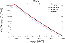
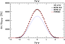
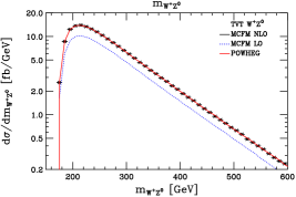
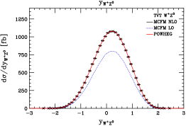
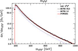
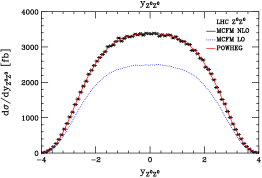
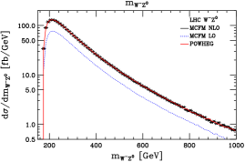
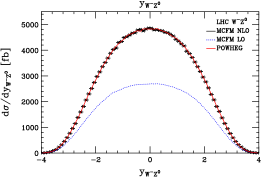
On the left of Fig. 1 we show the invariant mass of the weak boson system, , one of the Born variables for this process, for which there is excellent agreement between the Powheg result and that of Mcfm. Predictions for the Born variable, on the right-hand side of Fig. 1, are also seemingly indistinguishable from the corresponding Mcfm results. Recall that in the Powheg framework the Born variables are exactly preserved in the process of generating the hardest emission: they are distributed purely according to the function. Consequently, if the Powheg simulations and the underlying NLO calculations are implemented correctly these Born variables must agree exactly with fixed order NLO predictions. The results in Figure 1 already therefore constitute a very sensitive test of our implementation.
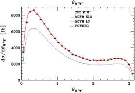
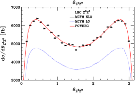
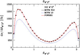
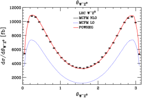
The distribution of the third Born variable is strongly reflected in Figure 2, which shows the polar angle between the incident parton traveling in the direction and the first of the produced vector bosons in their rest frame; in and production these are taken to be the and bosons respectively. This quantity is different to the Born variable in that the latter is defined as the polar angle of the first vector boson with respect to the quark in and collisions, and the gluon in collisions, which may or may not be traveling in the direction in the lab. Nevertheless, since this variable is fully inclusive and a close relative of the Born variable, , the level of agreement shown here between the Powheg and Mcfm predictions provides further strong assurance as to the correctness of our implementation. We add that we have also examined rapidity and pseudorapidity distributions of the individual vector bosons from our programs (not shown) which, like those in Figures 1 and 2, exhibit no discernible deviations from those given by Mcfm.
In Figure 3 we have displayed a number of distributions sensitive to the details of the decays of the vector bosons, specifically, the polar angle of one of the leptons produced by one of the decaying, resonant, vector bosons in its rest frame and, separately, the corresponding transverse momentum spectra. In all cases the agreement between our predictions and those of Mcfm is remarkably good. It is interesting to note that although our simulation only includes spin correlation effects in the leading order and real emission contributions to the cross section, it nevertheless reproduces very well the distributions predicted by Mcfm, which also includes the effects of NLO virtual corrections at the level of the spin correlations. Corroborating evidence for such behaviour can be found in the work of Grazzini [92, 93], whose calculations dealt with full NLO corrections to spin correlation matrices together with soft gluon resummation effects.
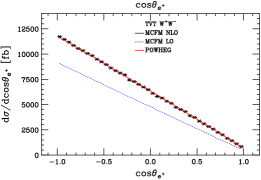
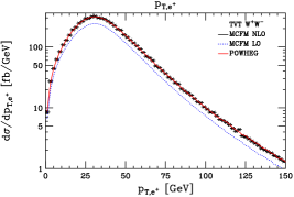
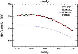
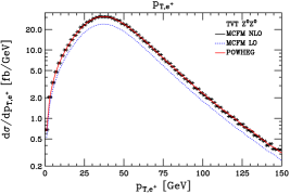
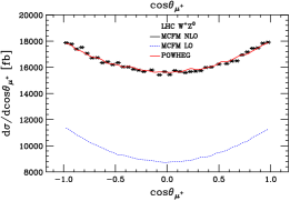
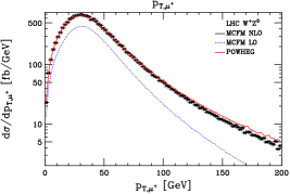
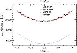
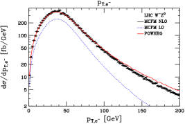
Actually, at Tevatron energies we find that the leading order production spin density matrix, calculated using the underlying Born kinematics , yields more-or-less identical distributions to those shown in Figure 3, on the contrary, at the LHC this somewhat naive procedure produces distributions close in shape to the leading order prediction, which is markedly different to the NLO one. These observations are very much in keeping with others in the literature [50], suggesting that virtual corrections to spin correlation matrices are typically small, whereas real emission corrections (which are generally larger at the LHC than at the Tevatron) can lead to sizeable effects.
Finally we wish to draw attention to the tails of the lepton distributions. In Figure 3 we see that for distributions forecast at Tevatron energies the Powheg and Mcfm predictions agree very well over the whole spectrum, whereas at the LHC we see that the two distributions overlap identically in the low region but in the high region the Powheg result is approximately 30% above that of Mcfm.
In fact this level of disagreement with respect to fixed order NLO predictions, in this region of phase space, is not unexpected. Events in which the final-state leptons have very high transverse momenta will, by their nature, typically contain associated high energy QCD radiation; this fact is substantiated by the shape of the corresponding leading order predictions shown in the blue dotted lines. Recall that, in the Powheg hardest emission cross section, the term responsible for the generation of the radiative variables is not simply equal to the NLO real emission cross section, but rather the NLO real emission cross section multiplied by a factor and the Sudakov form factor. In the high limit the latter factor tends to one, hence, Powheg events with high transverse momentum are generated according to the NLO real emission cross section multiplied by . Loosely speaking this factor is characteristic of the NLO total cross section K-factor, thus one expects the rate of events including high emissions to be different in Powheg with respect to a pure NLO calculation by such an amount (different by terms beyond NLO accuracy). This is indeed what we observe in Figure 3. Finally we add that the Born variables are unique exceptions to this reasoning since they are fully preserved, by construction, when radiation is generated, hence, unlike other inclusive observables the Born variables will always exactly equal the NLO prediction, regardless of whether the events are associated to high emissions or not.
4.2 Exclusive observables
In this section we shift the focus of our validation onto observables which more directly assess the generation of the hardest emission (Sect. 3.1) and additional radiation arising from the subsequent vetoed and truncated showers (Sect. 3.3). To this end we compare our results to two different approaches, namely, the default angular-ordered parton shower simulation in Herwig++ and also Mc@nlo v3.4 [94]. Since the latter program matches the same NLO matrix elements with the older Herwig parton shower [95, 96] it is formally of equivalent accuracy to our Powheg simulation, on the other hand, the former includes only LO matrix elements, hence, it is anticipated that it will fail to adequately model high radiation.
All of the results presented in this subsection, from each of the three approaches, were obtained at the parton level, after parton showering. The predictions from our Powheg simulation within Herwig++ are displayed as red dashed lines, while those of Mc@nlo and Herwig++ with the Powheg feature disabled are shown as black and blue dotted lines respectively.
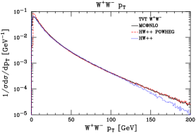
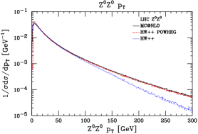
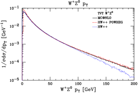
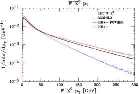
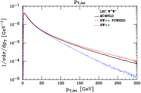
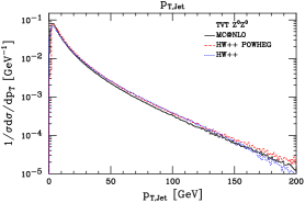
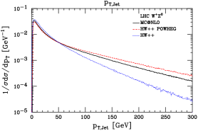
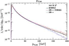
Figures 4 and 5 exhibit the transverse momentum spectra of the di-vector boson system and the hardest emitted jet. These distributions directly reflect the dependence of the hardest emission cross section Eq. 1, modulo small smearing effects due to the truncated and vetoed parton showers. All three approaches are seen to agree well in the low regions, where the parton shower approximation is expected to be reliable. In the high regions one can see that in all cases the parton shower by itself underestimates the production rate with respect to Mc@nlo and Powheg, moreover, we note that the degree to which it is underestimated is worse at LHC energies, than at the Tevatron, where the available phase space is more constrained (cf. Fig. 1).
In general the degree of overlap between the Mc@nlo and Powheg results is quite good, with differences between the two sets of predictions only being noticeable in the high tails for LHC energies. Such behavior has already been observed, and its nature well documented, in publications concerning other Powheg simulations [55, 56]; it is basically a further manifestation of the effect discussed at the end of Section 4.1, namely, that the distribution of the hardest emission in the Powheg method (Eq. 1) is given by multiplied by the NLO real emission cross section, whereas in Mc@nlo it is given by the real emission cross section alone. It follows that the Powheg predictions tend to exceed those of Mc@nlo and fixed order calculations when is large, by a factor of the order of the NLO total cross section K-factor. In keeping with this one sees that the relative differences seen in the tails of the transverse momentum spectra reflect the size of the relevant K-factors (cf. Fig. 1) and, accordingly, they are somewhat larger at the LHC than at the Tevatron.
Note that within the Powheg formalism it is possible to introduce so-called damping factors [55], which act in such a way as to reduce the effects of the multiplicative term, leading to cross sections in the high domain closer to those of fixed order calculations. However, there is no theoretical motivation to implement, or not to implement such damping, since the contribution from this factor, in the regions of phase space corresponding to high emission, is formally subleading – the differences with respect to Mc@nlo and fixed order predictions being indicative of the associated theoretical uncertainties.
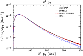
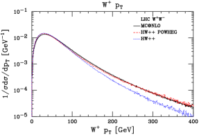
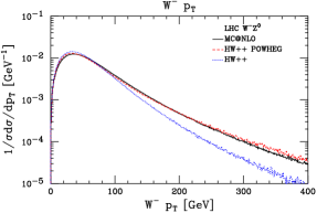
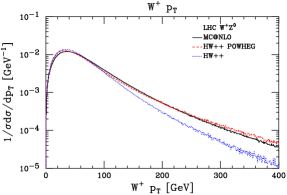
In Figure 6 we plot the transverse momentum spectra of individual vector bosons in each of the weak boson pair production channels, at nominal LHC energies only. In contrast to the transverse momentum spectrum of the diboson system, in fixed order perturbation theory this observable receives contributions at leading order for all values of . Thus one expects that any differences between the leading and next-to-leading parton shower predictions should be small, of order . It is then remarkable that these distributions show the next-to-leading order parton shower predictions, in good agreement with one another, exceeding the leading order parton shower prediction by up to a factor of four at high .
This curious result has already been noted and investigated in the original calculation of the fixed order NLO corrections to production in Ref. [32]. The same effect was subsequently observed in the case of production and subject to the same analysis in Ref. [33]. The detailed studies carried out in these publications conclude that the enhancement seen at high is greatly dominated by contributions arising from initiated real emission corrections. The reason for this large contribution was considered to be twofold. Firstly, it was noted that the luminosity for the channel was more than one order of magnitude greater than that of the channel at the LHC; secondly, in reactions, when the radiated quark and one of the weak bosons are produced with sufficiently high transverse momenta, the other weak boson may be produced as a ‘soft’ emission from the recoiling quark – a process which carries a large logarithmic enhancement factor, . It is further noted in Ref. [33] that fewer partonic subprocesses can participate in this enhancement mechanism in the case of production than in production, accordingly, we observe that the magnitude of the effect is somewhat smaller in the latter case.
Having studied several spectra we now turn to examine other distributions sensitive to the generation of the radiative variables and subsequent parton showering. As noted in earlier works concerning Higgs boson production, Ref. [56], the rapidity correlation between the leading jet and the recoiling colourless system is an interesting observable to examine from this point of view: for the case of a single hard emission the rapidity correlation can be expressed purely in terms of . In order to provide some additional physical insight regarding the nature of this quantity, we note that in the limit where the radiated parton is produced in the region perpendicular to the colliding beam partons, in the partonic centre-of-mass frame
| (40) |
where denotes the polar angle of the emitted parton in that frame. Furthermore, when the radiated parton is emitted along the directions, tends to .
In Figure 7 we show predictions for distributions in production and production at the Tevatron and LHC respectively. For each process we have considered how the results are affected by varying the cut on the leading jet. The general trends seen in these plots are qualitatively the same as those obtained in Higgs boson production and Higgs boson production in association with a boson [56], so too are our conclusions relating to them.
We remind the reader that, in general, parton shower Monte Carlo programs may not populate the full real emission phase space, resulting in so-called dead-zones. This is certainly true of the Herwig and Herwig++ simulations. The presence of dead zones in the real emission phase space follows directly from the scale choice used to initiate the parton shower evolution666For explicit phase space computations and maps concerning the origin of dead zones and their connection to the choice of the initial evolution scales see Refs. [83, 56, 97]., moreover, they are typically located in regions of phase space associated with high emissions. In Herwig and Herwig++ the dead zone for the first emission in processes such as this, comprised of a single initial-state colour dipole, is centred on , moreover, the angular breadth of the dead zone increases symmetrically and monotonically about this point with the energy of the emitted radiation (see e.g. Fig. 7 of Ref. [56]). The dip feature seen in the ordinary parton shower results (blue dots) directly reflects the angular characteristics of this unpopulated region of phase space: in all cases, as the cut on the leading jet increases the dip becomes broader and deeper.
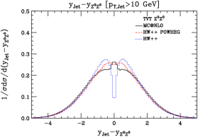
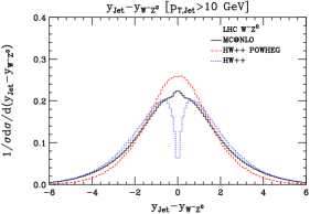
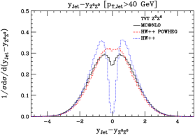
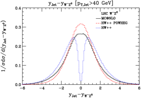
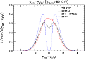
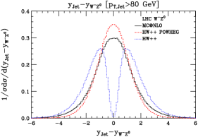
Since Mc@nlo and Powheg aim to fully include NLO corrections within the parton shower simulation, they naturally populate all of the real emission phase space. In keeping with this, we observe that the predictions from these two approaches do not show the same significant dip in the central region of the distributions. Whereas the Powheg simulation fills this phase space independently of the detailed workings of the parton shower to which it is subsequently attached, the Mc@nlo approach involves carefully augmenting the parton shower simulation by the difference between its own approximate real emission cross section and the true real emission cross section in the NLO calculation. In particular, this means that the distribution of radiation from Mc@nlo in the dead zone follows exactly the fixed order NLO calculation, while either side of it the distribution differs from this by terms.
Having noted this NNLO discontinuity in the radiation pattern, it is then understandable that the Mc@nlo predictions (black) can exhibit some minor irregularities and differences with respect to Powheg (red) in the central region and that these should reflect, somewhat, the trends seen in the results obtained using the parton shower alone. On the contrary, the response of the Powheg predictions to the increasing cut on the leading jet lends itself to a more straightforward interpretation based on simple kinematic reasoning, namely, that the distribution should become more central, as the phase space available for small angle emissions – which populate the tails – becomes reduced relative to that available for large angle emissions. Furthermore, we point out that for observables employing cuts which exclude the softer regions of phase space, such as with a cut of 80 GeV on the leading jet, one expects that the Powheg predictions exceed those of conventional NLO calculations due to the factor multiplying the real emission cross section in Eq. 1. This behaviour is apparent in Figure 7. Finally, we remark that we have reproduced all of these distributions using our Powheg simulation with the truncated shower feature disabled, with no observable consequences.
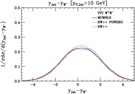
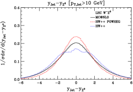
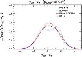
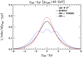
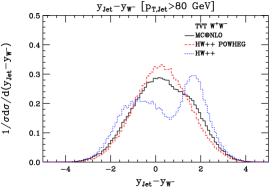
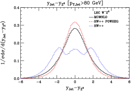
Figure 8 shows the differences in rapidity between the leading jet and one of the vector bosons in production at the Tevatron and production at the LHC. Since these distributions are closely related to those in Fig. 7, we argue that the differences seen in the leading order parton shower predictions with respect to Mc@nlo and Powheg are again attributable to the dead zone in the former; a fortiori considering the variation of the uncorrected parton shower results with respect to the changing cut on the leading jet. We contend that the peculiar shape of the pure parton shower results reflect the impression left by the dead zone in convoluted with the rapidity distribution of the vector bosons with respect to one another. In all of the distributions the agreement between the Mc@nlo and Powheg results is quite satisfactory: note that both approaches formally only offer a leading order description of this quantity. Some small distortion can be seen on the right of the Mc@nlo distribution at the Tevatron, for a cut of GeV on the leading jet, which we tentatively suggest is indicative of the asymmetric parton shower prediction.
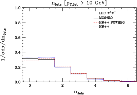
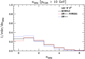
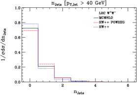
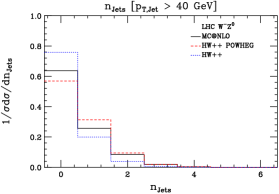
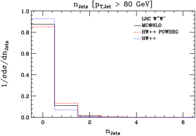
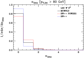
LHC predictions for jet multiplicity distributions in and production can be found in Figure 9, assuming a hadronic centre-of-mass energy of 14 TeV. As one expects, in all cases jet multiplicities decrease rapidly as the cut on the leading jet is increased. One can also see that the results obtained using the parton shower alone show a tendency to overestimate the number of events without any jets in comparison to the other methods. This is also expected given our earlier discussions concerning the dead zone in the parton shower phase space. Finally we note that the Powheg predictions for the number of events with one jet are above those of Mc@nlo by an amount characteristic of the NLO K-factor. As noted previously, this systematic effect can be directly attributed to the presence of the factor multiplying the real emission part of the Powheg hardest emission cross section (Eq. 1). Once again we note that the presence of this term modifies the distribution of hard radiation by terms of NNLO significance only.
5 Conclusion
In this article we have presented an implementation of the Powheg NLO matching formalism for simulations of weak boson pair production and decay, in the double pole approximation. These simulations have been integrated within the Herwig++ Monte Carlo event generator, including truncated shower effects to account for colour coherence phenomena.
In constructing this NLO event generator we have employed novel relations between the cross sections and those of and production. Total cross sections and parton level NLO distributions were found to be in excellent agreement with predictions obtained from the the Mcfm NLO Monte Carlo program.
The shapes of the emission spectra from the full simulation, including parton shower effects, are seen to generally compare well with those of Mc@nlo in a wide variety of kinematic distributions – both of which exhibit large corrections with respect to the default parton shower predictions. Where minor differences have arisen between our results and Mc@nlo they have been studied in detail.
As noted in previous works comparing Mc@nlo and Powheg [55, 56] we observe a tendency for Powheg to produce slightly more hard radiation than Mc@nlo. The explanation given for this effect in those publications is seen to hold well here, specifically, that the factor which multiplies the real part of the Powheg hardest emission cross section leads to an enhancement of high radiation with respect to the corresponding NLO prediction; the differences being formally of order . As in Refs. [55, 56] we also find that the Mc@nlo program exhibits a sensitivity to the phase space partitioning in the underlying parton shower simulation (cf. Figs. 7 and 8), however, as with the enhancement of hard radiation in Powheg, this is formally representative of NNLO effects.
All weak boson boson pair production simulations presented here are due for inclusion in the next public release of the Herwig++ event generator.
Acknowledgments.
I wish to thank my colleagues in the Herwig++ and Powheg-Box collaborations for valuable input in the course of this work. I am also very grateful to Pavel Demin, Fabio Maltoni and the rest of CP3 Louvain for providing access to their high performance computing cluster.Appendix A Regularized and unregularized splitting functions
We write the ‘customary’ regularized Altarelli-Parisi functions in terms of -distributions as
where
and
with all other and being equal to zero.
References
- [1] ALEPH Collaboration et. al., Precision Electroweak Measurements and Constraints on the Standard Model, arXiv:0811.4682.
- [2] ALEPH Collaboration, R. Barate et. al., Measurement of W pair production in e+ e- collisions at 189-GeV, Phys. Lett. B484 (2000) 205–217, [hep-ex/0005043].
- [3] DELPHI Collaboration, P. Abreu et. al., W pair production cross-section and W branching fractions in e+ e- interactions at 189-GeV, Phys. Lett. B479 (2000) 89–100, [hep-ex/0103013].
- [4] L3 Collaboration, M. Acciarri et. al., Measurement of the pair production cross-section and decay branching fractions in interactions at = 189-GeV, Phys. Lett. B496 (2000) 19–33, [hep-ex/0008026].
- [5] OPAL Collaboration, G. Abbiendi et. al., W+ W- production cross section and W branching fractions in e+ e- collisions at 189-GeV, Phys. Lett. B493 (2000) 249–265, [hep-ex/0009019].
- [6] S. Natale, W and Z pair production at LEP2, Eur. Phys. J. C33 (2004) s706–s708.
- [7] D0 Collaboration, V. M. Abazov et. al., Measurement of the production cross section in collisions at TeV, Phys. Rev. Lett. 94 (2005) 151801, [hep-ex/0410066].
- [8] D0 Collaboration, V. M. Abazov et. al., Production of WZ events in collisions at = 1.96-TeV and limits on anomalous WWZ couplings, Phys. Rev. Lett. 95 (2005) 141802, [hep-ex/0504019].
- [9] CDF Collaboration, D. E. Acosta et. al., Measurement of the production cross section in collisions at TeV using dilepton events, Phys. Rev. Lett. 94 (2005) 211801, [hep-ex/0501050].
- [10] D0 Collaboration, V. M. Abazov et. al., Measurement of the cross-section at = 1.96-TeV and limits on WWZ trilinear gauge couplings, Phys. Rev. D76 (2007) 111104, [arXiv:0709.2917].
- [11] CDF Collaboration, A. Abulencia et. al., Observation of Production, Phys. Rev. Lett. 98 (2007) 161801, [hep-ex/0702027].
- [12] CDF Collaboration, T. Aaltonen et. al., First Observation of Vector Boson Pairs in a Hadronic Final State at the Tevatron Collider, Phys. Rev. Lett. 103 (2009) 091803, [arXiv:0905.4714].
- [13] CDF Collaboration, T. Aaltonen et. al., Measurement of the Production Cross Section and Search for Anomalous and Couplings in Collisions at TeV, Phys. Rev. Lett. 104 (2010) 201801, [arXiv:0912.4500].
- [14] D0 Collaboration, V. M. Abazov et. al., Measurement of trilinear gauge boson couplings from WW + WZ to lnu jj events in pp-bar collisions at sqrts=1.96 TeV, Phys. Rev. D80 (2009) 053012, [arXiv:0907.4398].
- [15] CDF Collaboration, T. Aaltonen et. al., Measurement of the Production Cross Section Using a Matrix Element Technique in Lepton + Jets Events, arXiv:1008.4404.
- [16] J. Ellison and J. Wudka, Study of trilinear gauge boson couplings at the Tevatron collider, Ann. Rev. Nucl. Part. Sci. 48 (1998) 33–80, [hep-ph/9804322].
- [17] The TEVNPH Working Group of the CDF and D0 Collaboration, Combined CDF and D0 Upper Limits on Standard Model Higgs- Boson Production with up to 6.7 fb-1 of Data, arXiv:1007.4587.
- [18] T. G. Rizzo, DECAYS OF HEAVY HIGGS BOSONS, Phys. Rev. D22 (1980) 722.
- [19] W.-Y. Keung and W. J. Marciano, HIGGS SCALAR DECAYS: H W+- X, Phys. Rev. D30 (1984) 248.
- [20] E. Eichten, I. Hinchliffe, K. D. Lane, and C. Quigg, Super Collider Physics, Rev. Mod. Phys. 56 (1984) 579–707.
- [21] A. Djouadi, J. Kalinowski, and P. M. Zerwas, Two- and Three-Body Decay Modes of SUSY Higgs Particles, Z. Phys. C70 (1996) 435–448, [hep-ph/9511342].
- [22] Higgs Working Group Collaboration, M. S. Carena et. al., Report of the Tevatron Higgs working group, hep-ph/0010338.
- [23] J. F. Gunion, H. E. Haber, G. L. Kane, and S. Dawson, The Higgs Hunter’s Guide, . SCIPP-89/13.
- [24] M. S. Chanowitz and W. B. Kilgore, and backgrounds to strong scattering at the LHC, Phys. Lett. B347 (1995) 387–393, [hep-ph/9412275].
- [25] K. T. Matchev and D. M. Pierce, Supersymmetry reach of the Tevatron via trilepton, like sign dilepton and dilepton plus jet signatures, Phys. Rev. D60 (1999) 075004, [hep-ph/9904282].
- [26] H. Baer, M. Drees, F. Paige, P. Quintana, and X. Tata, Trilepton signal for supersymmetry at the Fermilab Tevatron revisited, Phys. Rev. D61 (2000) 095007, [hep-ph/9906233].
- [27] ATLAS detector and physics performance. Technical design report. Vol. 2, . CERN-LHCC-99-15.
- [28] B. Mele, P. Nason, and G. Ridolfi, QCD radiative corrections to Z boson pair production in hadronic collisions, Nucl. Phys. B357 (1991) 409–438.
- [29] J. Ohnemus and J. F. Owens, An Order calculation of hadronic production, Phys. Rev. D43 (1991) 3626–3639.
- [30] J. Ohnemus, An Order calculation of hadronic production, Phys. Rev. D44 (1991) 1403–1414.
- [31] J. Ohnemus, An Order calculation of hadronic production, Phys. Rev. D44 (1991) 3477–3489.
- [32] S. Frixione, P. Nason, and G. Ridolfi, Strong corrections to WZ production at hadron colliders, Nucl. Phys. B383 (1992) 3–44.
- [33] S. Frixione, A Next-to-leading order calculation of the cross-section for the production of pairs in hadronic collisions, Nucl. Phys. B410 (1993) 280–324.
- [34] L. J. Dixon, Z. Kunszt, and A. Signer, Helicity amplitudes for O(alpha-s) production of , , , , or pairs at hadron colliders, Nucl. Phys. B531 (1998) 3–23, [hep-ph/9803250].
- [35] L. J. Dixon, Z. Kunszt, and A. Signer, Vector boson pair production in hadronic collisions at order : Lepton correlations and anomalous couplings, Phys. Rev. D60 (1999) 114037, [hep-ph/9907305].
- [36] J. M. Campbell and R. K. Ellis, An update on vector boson pair production at hadron colliders, Phys. Rev. D60 (1999) 113006, [hep-ph/9905386].
- [37] S. Catani, F. Krauss, R. Kuhn, and B. R. Webber, QCD Matrix Elements + Parton Showers, JHEP 11 (2001) 063, [hep-ph/0109231].
- [38] F. Krauss, Matrix Elements and Parton Showers in Hadronic Interactions, JHEP 08 (2002) 015, [hep-ph/0205283].
- [39] A. Schälicke and F. Krauss, Implementing the ME+PS Merging Algorithm, JHEP 07 (2005) 018, [hep-ph/0503281].
- [40] L. Lönnblad, Correcting the Colour-Dipole Cascade Model with Fixed Order Matrix Elements, JHEP 05 (2002) 046, [hep-ph/0112284].
- [41] M. L. Mangano, M. Moretti, and R. Pittau, Multijet Matrix Elements and Shower Evolution in Hadronic Collisions: jets as a Case Study, Nucl. Phys. B632 (2002) 343–362, [hep-ph/0108069].
- [42] S. Mrenna and P. Richardson, Matching Matrix Elements and Parton Showers with HERWIG and PYTHIA, JHEP 05 (2004) 040, [hep-ph/0312274].
- [43] S. Frixione and B. R. Webber, Matching NLO QCD Computations and Parton Shower Simulations, JHEP 06 (2002) 029, [hep-ph/0204244].
- [44] P. Nason, A New Method for Combining NLO QCD with Shower Monte Carlo Algorithms, JHEP 11 (2004) 040, [hep-ph/0409146].
- [45] S. Frixione, P. Nason, and C. Oleari, Matching NLO QCD Computations with Parton Shower Simulations: the POWHEG Method, JHEP 11 (2007) 070, [arXiv:0709.2092].
- [46] S. Frixione, P. Nason, and B. R. Webber, Matching NLO QCD and Parton Showers in Heavy flavour Production, JHEP 08 (2003) 007, [hep-ph/0305252].
- [47] S. Frixione, E. Laenen, P. Motylinski, and B. R. Webber, Single-top Production in MC@NLO, JHEP 03 (2006) 092, [hep-ph/0512250].
- [48] S. Frixione and B. R. Webber, The MC@NLO 3.3 Event Generator, hep-ph/0612272.
- [49] S. Frixione, E. Laenen, P. Motylinski, B. Webber, and C. D. White, Single-top Hadroproduction in Association with a W Boson, arXiv:0805.3067.
- [50] S. Frixione, E. Laenen, P. Motylinski, and B. R. Webber, Angular Correlations of Lepton Pairs from Vector Boson and Top Quark Decays in Monte Carlo Simulations, JHEP 04 (2007) 081, [hep-ph/0702198].
- [51] S. Frixione, P. Nason, and G. Ridolfi, A Positive-Weight Next-to-Leading-Order Monte Carlo for Heavy Flavour Hadroproduction, JHEP 09 (2007) 126, [arXiv:0707.3088].
- [52] S. Frixione, P. Nason, and G. Ridolfi, The POWHEG-hvq Manual Version 1.0, arXiv:0707.3081.
- [53] S. Alioli, P. Nason, C. Oleari, and E. Re, NLO vector-boson production matched with shower in POWHEG, JHEP 07 (2008) 060, [arXiv:0805.4802].
- [54] K. Hamilton, P. Richardson, and J. Tully, A Positive-Weight Next-to-Leading Order Monte Carlo Simulation of Drell-Yan Vector Boson Production, arXiv:0806.0290.
- [55] S. Alioli, P. Nason, C. Oleari, and E. Re, NLO Higgs boson production via gluon fusion matched with shower in POWHEG, arXiv:0812.0578.
- [56] K. Hamilton, P. Richardson, and J. Tully, A Positive-Weight Next-to-Leading Order Monte Carlo Simulation for Higgs Boson Production, JHEP 04 (2009) 116, [arXiv:0903.4345].
- [57] S. Alioli, P. Nason, C. Oleari, and E. Re, NLO single-top production matched with shower in POWHEG: s- and t-channel contributions, JHEP 09 (2009) 111, [arXiv:0907.4076].
- [58] P. Nason and C. Oleari, NLO Higgs boson production via vector-boson fusion matched with shower in POWHEG, JHEP 02 (2010) 037, [arXiv:0911.5299].
- [59] S. Alioli, P. Nason, C. Oleari, and E. Re, A general framework for implementing NLO calculations in shower Monte Carlo programs: the POWHEG BOX, JHEP 06 (2010) 043, [arXiv:1002.2581].
- [60] P. Nason and G. Ridolfi, A Positive-Weight Next-to-leading-Order Monte Carlo for Z pair Hadroproduction, JHEP 08 (2006) 077, [hep-ph/0606275].
- [61] R. Frederix, S. Frixione, F. Maltoni, and T. Stelzer, Automation of next-to-leading order computations in QCD: the FKS subtraction, JHEP 10 (2009) 003, [arXiv:0908.4272].
- [62] S. Hoeche, F. Krauss, M. Schonherr, and F. Siegert, Automating the POWHEG method in Sherpa, arXiv:1008.5399.
- [63] CDF Collaboration, T. Aaltonen et. al., First Measurement of Production in panti-p Collisions at = 1.96-TeV, Phys. Rev. Lett. 100 (2008) 201801, [arXiv:0801.4806].
- [64] D0 Collaboration, V. M. Abazov et. al., Observation of production in collisions at = 1.96-TeV, Phys. Rev. Lett. 101 (2008) 171803, [arXiv:0808.0703].
- [65] D0 Collaboration, V. M. Abazov et. al., Search for a resonance decaying into WZ boson pairs in collisions, Phys. Rev. Lett. 104 (2010) 061801, [arXiv:0912.0715].
- [66] The CDF Collaboration, T. Aaltonen et. al., Search for and resonances decaying to electron, missing , and two jets in collisions at TeV, Phys. Rev. Lett. 104 (2010) 241801, [arXiv:1004.4946].
- [67] V. Brigljevic et. al., Study of di-boson production with the CMS detector at LHC, J. Phys. G34 (2007) N269–N295.
- [68] CDF Collaboration, T. Aaltonen et. al., Limits on Anomalous Triple Gauge Couplings in Collisions at = 1.96-TeV, Phys. Rev. D76 (2007) 111103, [arXiv:0705.2247].
- [69] D0 Collaboration, V. M. Abazov et. al., Combined measurements of anomalous charged trilinear gauge-boson couplings from diboson production in p-pbar collisions at sqrt(s)=1.96 TeV, arXiv:0907.4952.
- [70] CDF Collaboration, T. Aaltonen et. al., Improved Search for a Higgs Boson Produced in Association with Z->l+l- in proton antiproton Collisions at sqrt(s) = 1.96 TeV, arXiv:1009.3047.
- [71] CDF and D0 Collaboration, T. Aaltonen et. al., Combination of Tevatron searches for the standard model Higgs boson in the W+W- decay mode, Phys. Rev. Lett. 104 (2010) 061802, [arXiv:1001.4162].
- [72] The CDF Collaboration, T. Aaltonen et. al., Inclusive Search for Standard Model Higgs Boson Production in the WW Decay Channel using the CDF II Detector, Phys. Rev. Lett. 104 (2010) 061803, [arXiv:1001.4468].
- [73] The D0 Collaboration, V. M. Abazov et. al., Search for Higgs boson production in dilepton and missing energy final states with 5.4 of collisions at TeV, Phys. Rev. Lett. 104 (2010) 061804, [arXiv:1001.4481].
- [74] M. Bähr et. al., Herwig++ 2.2 Release Note, arXiv:0804.3053.
- [75] M. Bähr et. al., Herwig++ Physics and Manual, arXiv:0803.0883.
- [76] M. L. Mangano, P. Nason, and G. Ridolfi, Heavy quark correlations in hadron collisions at next-to- leading order, Nucl. Phys. B373 (1992) 295–345.
- [77] S. Catani and M. H. Seymour, A general algorithm for calculating jet cross sections in NLO QCD, Nucl. Phys. B485 (1997) 291–419, [hep-ph/9605323].
- [78] E. Re, Single-top Wt-channel production matched with parton showers using the POWHEG method, arXiv:1009.2450.
- [79] L. Lönnblad, ThePEG, PYTHIA7, Herwig++ and ARIADNE, Nucl. Instrum. Meth. A559 (2006) 246–248.
- [80] H. Murayama, I. Watanabe, and K. Hagiwara, HELAS: HELicity amplitude subroutines for Feynman diagram evaluations, . KEK-91-11.
- [81] T. Sjöstrand, S. Mrenna, and P. Skands, PYTHIA 6.4 Physics and Manual, JHEP 05 (2006) 026, [hep-ph/0603175].
- [82] Y. L. Dokshitzer, D. Diakonov, and S. I. Troian, Hard Processes in Quantum Chromodynamics, Phys. Rept. 58 (1980) 269–395.
- [83] S. Gieseke, P. Stephens, and B. Webber, New Formalism for QCD Parton Showers, JHEP 12 (2003) 045, [hep-ph/0310083].
- [84] K. Hamilton, P. Richardson, and J. Tully, A modified CKKW matrix element merging approach to angular-ordered parton showers, JHEP 11 (2009) 038, [arXiv:0905.3072].
- [85] A. D. Martin, R. G. Roberts, W. J. Stirling, and R. S. Thorne, Uncertainties of Predictions from Parton Distributions. I: Experimental errors, Eur. Phys. J. C28 (2003) 455–473, [hep-ph/0211080].
- [86] M. R. Whalley, D. Bourilkov, and R. C. Group, The Les Houches Accord PDFs (LHAPDF) and Lhaglue, hep-ph/0508110.
- [87] S. D. Ellis and D. E. Soper, Successive combination jet algorithm for hadron collisions, Phys. Rev. D48 (1993) 3160–3166, [hep-ph/9305266].
- [88] S. Catani, Y. L. Dokshitzer, M. H. Seymour, and B. R. Webber, Longitudinally invariant clustering algorithms for hadron hadron collisions, Nucl. Phys. B406 (1993) 187–224.
- [89] M. Cacciari and G. P. Salam, Dispelling the myth for the jet-finder, Phys. Lett. B641 (2006) 57–61, [hep-ph/0512210].
- [90] J. M. Campbell and R. K. Ellis, Radiative Corrections to production, Phys. Rev. D62 (2000) 114012, [hep-ph/0006304].
- [91] J. M. Campbell, R. K. Ellis, and G. Zanderighi, Next-to-leading order Higgs + 2 jet production via gluon fusion, JHEP 10 (2006) 028, [hep-ph/0608194].
- [92] M. Grazzini, Soft-gluon effects in W W production at hadron colliders, JHEP 01 (2006) 095, [hep-ph/0510337].
- [93] R. Frederix and M. Grazzini, Higher-order QCD effects in the h to ZZ search channel at the LHC, Phys. Lett. B662 (2008) 353–359, [arXiv:0801.2229].
- [94] S. Frixione and B. R. Webber, The MC@NLO 3.4 Event Generator, arXiv:0812.0770.
- [95] G. Corcella et. al., HERWIG 6: An Event Generator for Hadron Emission Reactions With Interfering Gluons (including supersymmetric processes), JHEP 01 (2001) 010, [hep-ph/0011363].
- [96] G. Corcella et. al., HERWIG 6.5 Release Note, hep-ph/0210213.
- [97] P. Torrielli and S. Frixione, Matching NLO QCD computations with PYTHIA using MC@NLO, JHEP 04 (2010) 110, [arXiv:1002.4293].