Abstract

We evaluate the radion and Higgs masses in the gauge-Higgs unification models on the warped geometry, in which the modulus is stabilized by the Casimir energy. We analyze the one-loop effective potential and clarify the dependences of those masses on the Wilson line phase $\theta_{\rm H}$. The radion mass varies 1-30 GeV for $0.06\leq\sin\theta_{\rm H}\leq 0.3$, while the Higgs mass is 150-200 GeV and depends on $\theta_{\rm H}$ only logarithmically. The radion couplings to the standard model particles are sensitive to the warp factor, and are too small to detect at colliders in the region where the five-dimensional description is valid.

January 22, 2011

KEK-TH-1402

1 Introduction

The gauge-Higgs unification scenario is an interesting candidate for the physics beyond the standard model, which was originally proposed in Refs. [1, 2] and revived by Refs. [3, 4] as a solution to the naturalness problem. In this class of models, the Higgs mass is protected against large radiative corrections thanks to a higher-dimensional gauge symmetry [5]. The models are characterized by the Wilson line phase along the extra dimension $\theta_{\rm H}$. The electroweak symmetry breaking occurs when $\sin\theta_{\rm H}\neq 0$ or $\sin\frac{\theta_{\rm H}}{2}\neq 0$, depending on the models. The fluctuation around the vacuum expectation value (VEV) of $\theta_{\rm H}$ corresponds to the physical Higgs boson in the standard model.

This scenario has been first investigated in the flat spacetime [6, 7], and extended to the Randall-Sundrum warped spacetime [8]. The models in the latter can solve some problems that exist in the former case. The masses of the Higgs and the Kaluza-Klein (KK) modes are enhanced by a logarithm of the large warp factor [9] so that they can evade the experimental lower bounds, and the large top quark mass can easily be realized only by the localization of the mode functions in the extra dimension [10]. Furthermore, such models have phenomenologically interesting features [10]-[16]. Hence, we will focus on the Randall-Sundrum spacetime as a background geometry in this paper.

When we work in extra-dimensional models, the stabilization mechanism for the size of the extra dimension, which is often called the modulus or the radion, must be considered. One of the simplest mechanisms for the modulus stabilization is proposed in Ref. [17]. A five-dimensional (5D) bulk scalar field plays an essential role for the stabilization in this mechanism. The modulus can also be stabilized by the Casimir energy of the bulk fields. This possibility has been discussed in many papers [18]-[21], and it has been shown that 5D gauge and fermion fields that spread over the bulk are essential for the modulus stabilization [22]. Thus the latter mechanism is more economical in the gauge-Higgs unification scenario because the bulk gauge and fermion fields already exist in the theory and no extra bulk scalar fields need not be introduced just for the stabilization.

In our previous work [23], we discussed the modulus stabilization by the Casimir energy in the model proposed in Ref. [14], in which the Wilson line phase is dynamically determined as $\theta_{\rm H}=\frac{\pi}{2}$. We found there that the brane kinetic terms for the gauge fields are necessary for the modulus stabilization, and the radion mass is ${\cal O}(1~{}\mbox{GeV})$. Although this model has phenomenologically interesting features [16], the electroweak precision measurements disfavor $\theta_{\rm H}=\frac{\pi}{2}$ according to the analysis in Ref. [10]. Besides, it is a nontrivial task to clarify the $\theta_{\rm H}$-dependence of the radion and Higgs masses because the effective potential $V_{\rm eff}$ depends on parameters that control the VEV of $\theta_{\rm H}$ in a complicated way. Therefore, in this paper, we will extend our previous work [23] to the case that $\theta_{\rm H}$ can take small values and clarify the $\theta_{\rm H}$-dependence of the radion and Higgs masses by evaluating $V_{\rm eff}$. We will also discuss the experimental constraints on the radion mass.

The paper is organized as follows. In the next section, we provide a brief review of the model in Ref. [14] focusing on the matter sector, and show the one-loop effective potential for the radion and Higgs fields. In Sec. 3, we extend the matter sector of the model to realize small values of $\theta_{\rm H}$, and see how the effective potential is modified by such extensions. In Sec. 4, we estimate the radion and Higgs masses as functions of $\theta_{\rm H}$, and comment on the experimental constraints on the radion mass. Sec. 5 is devoted to the summary. We define some functions useful for our analysis in Appendix A, show an approximate form of the effective potential in Appendix B, and provide some useful expressions for the numerical calculation in Appendix C.

2 $SO(5)\times U(1)_{X}$ model

In this paper, we consider the gauge-Higgs unification models based on a 5D $SO(5)\times U(1)_{X}$ gauge theory. This class of models was first discussed in Ref. [10], and several similar models with different matter sectors have been studied so far [11, 14, 25]. In our previous work [23], we considered a model proposed in Ref. [14] as the simplest example. We start with a brief review of this model, focusing on the matter sector, and extend it later.

We assume the 5D warped spacetime compactified on an orbifold $S^{1}/Z_{2}$ [8] as a background geometry. The background metric is given by

$$ds^{2}=G_{MN}dx^{M}dx^{N}=e^{-2\sigma(y)}\eta_{\mu\nu}dx^{\mu}dx^{\nu}+dy^{2},$$ (2.1)

where $M,N=0,1,2,3,4$ are 5D indices and $\eta_{\mu\nu}={\rm diag}(-1,1,1,1)$. The fundamental region of $S^{1}/Z_{2}$ is $0\leq y\leq L$. The function $e^{\sigma(y)}$ is a warp factor, and $\sigma(y)=ky$ in the fundamental region, where $k$ is the inverse AdS curvature radius. The orbifold has two fixed points $y=0$ and $y=L$, which are called the UV and IR branes, respectively. The gauge symmetry is broken to $SU(2)_{\rm L}\times SU(2)_{\rm R}\times U(1)_{X}$ at the IR brane, and to $SU(2)_{\rm L}\times U(1)_{Y}$ at the UV brane by boundary conditions [10]. In order to stabilize the modulus, we need brane-localized kinetic terms for the gauge fields [22]. Thus we introduce the following terms on the IR brane.

$${\cal L}_{\rm bd}^{\rm kin}=2\sqrt{-g}\left[-\frac{\kappa_{c}}{4k}{\rm tr}\left\{F_{\mu\nu}^{(G)}F^{(G)\mu\nu}\right\}-\frac{\kappa_{w}}{4k}{\rm tr}\left\{F_{\mu\nu}^{(A)}F^{(A)\mu\nu}\right\}-\frac{\kappa_{x}}{4k}F_{\mu\nu}^{(B)}F^{(B)\mu\nu}\right]\delta(y-L),$$ (2.2)

where $\sqrt{-g}\equiv\det(g_{\mu\nu})$, $g_{\mu\nu}$ is the 4D induced metric on the IR brane, $F_{MN}^{(G)}$, $F_{MN}^{(A)}$, $F_{MN}^{(B)}$ are field strengths for the $SU(3)_{C}$, $SO(5)$, $U(1)_{X}$ gauge fields, and $\kappa_{c}$, $\kappa_{w}$, $\kappa_{x}$ are dimensionless constants. For simplicity, we do not consider kinetic terms on the UV brane nor brane kinetic terms for the 5D fermions, and assume that $\kappa\equiv\kappa_{c}=\kappa_{w}=\kappa_{x}$ in the following.

2.1 Matter sector

We introduce 5D fermions $\Psi_{i}$ ($i=1,2,\cdots$) belonging to the vectorial representation of $SO(5)$ as matter fields. The 5D Lagrangian in this sector is given by

$${\cal L}=\sqrt{-G}\left[\sum_{i}\left\{i\bar{\Psi}_{i}\Gamma^{N}{\cal D}_{N}\Psi_{i}-iM_{\Psi i}\varepsilon(y)\bar{\Psi}_{i}\Psi_{i}\right\}+\cdots\right],$$ (2.3)

where $G\equiv\det(G_{MN})$, $\Gamma^{N}$ are 5D gamma matrices contracted by the fünfbein, ${\cal D}_{N}$ is the covariant derivative, and $\varepsilon(y)$ is a periodic step function. The ellipsis denotes the gauge sector.

It is useful to express the $SO(5)$ vector $\Psi=(\psi_{1},\cdots,\psi_{5})^{t}$ as

$$\Psi=\left[\begin{pmatrix}\hat{\psi}_{11}\\ \hat{\psi}_{21}\end{pmatrix},\;\begin{pmatrix}\hat{\psi}_{12}\\ \hat{\psi}_{22}\end{pmatrix},\;\psi_{5}\right],$$ (2.4)

where

$$\hat{\psi}=\begin{pmatrix}\hat{\psi}_{11}&\hat{\psi}_{12}\\ \hat{\psi}_{21}&\hat{\psi}_{22}\end{pmatrix}\equiv\frac{1}{\sqrt{2}}\left(\psi_{4}{\mbox{\boldmath$1_{2}$}}+i\vec{\psi}\cdot\vec{\sigma}\right)i\sigma_{2}$$ (2.5)

is a bidoublet and $\psi_{5}$ is a singlet for $SU(2)_{\rm L}\times SU(2)_{\rm R}$. For example, the third generation of the quark sector comes from two multiplets $\Psi_{1}$ and $\Psi_{2}$, which are expressed as

$$\Psi_{1}\!\!\! =\!\!\! \left[Q_{1}=\begin{pmatrix}T\\ B\end{pmatrix},\;q=\begin{pmatrix}t\\ b\end{pmatrix},\;t^{\prime}\right],$$

$$\Psi_{2}\!\!\! =\!\!\! \left[Q_{2}=\begin{pmatrix}U\\ D\end{pmatrix},\;Q_{3}=\begin{pmatrix}X\\ Y\end{pmatrix},\;b^{\prime}\right].$$ (2.6)

The orbifold parities for them are listed in Table I. The subscript $R$ denotes the 4D right-handed chirality defined by $\gamma_{5}\equiv\Gamma^{4}$. The left-handed components have the opposite parities to the right-handed ones.

$Q_{1R}$	$q_{R}$	$t^{\prime}_{R}$	$Q_{2R}$	$Q_{3R}$	$b^{\prime}_{R}$
$(-,-)$	$(-,-)$	$(+,+)$	$(-,-)$	$(-,-)$	$(+,+)$

Table I: The orbifold parities for the fermions. The left and the right signs in the parenthesis denote parities around $y=0$ and $y=L$, respectively. The left-handed components have the opposite parities to the right-handed ones.

On the UV brane, we can introduce brane-localized chiral fermion fields and change the boundary conditions there, just like we did in Ref. [14]. The resulting boundary conditions on the UV brane are

$$Q_{1L}=c_{\omega}q_{L}+s_{\omega}Q_{2L}=Q_{3L}=0,$$

$$-s_{\omega}q_{R}+c_{\omega}Q_{2R}=0,\;\;\;\;\;t^{\prime}_{L}=b^{\prime}_{L}=0,$$ (2.7)

at $y=0$. Here $s_{\omega}\equiv\sin\omega$, $c_{\omega}\equiv\cos\omega$, and $\omega$ is a mixing angle determined by the ratio of the boundary mass parameters. (Since $q_{L}$ and $Q_{2L}$ have the same quantum numbers for $SU(2)_{\rm L}\times U(1)_{Y}$, they can mix on the UV brane.)

2.2 Mass spectrum

The mass spectrum $\left\{m_{n}\right\}$ in the 4D effective theory is determined as solutions to the equation,

$$\rho^{I}(\lambda_{n};\theta_{\rm H})=0,$$ (2.8)

where $I$ specifies the sectors, and $\lambda_{n}\equiv m_{n}/k$. The functions $\rho^{I}(\lambda;\theta_{\rm H})$ are written in terms of the Bessel functions, and listed in Appendix A of Ref. [23]. (See (B.1), for example.)

The W and Z boson masses are obtained as the lightest solutions to $\rho^{W}(\lambda_{W};\theta_{\rm H})=0$ and $\rho^{Z}(\lambda_{Z};\theta_{\rm H})=0$, and are approximately expressed as

$$m_{W}\!\!\! =\!\!\! k\lambda_{W}\simeq\frac{ke^{-kL}\sin\theta_{\rm H}}{\sqrt{kL+\kappa}},$$

$$m_{Z}\!\!\! =\!\!\! k\lambda_{Z}\simeq\sqrt{\frac{1+s_{\phi}^{2}}{kL+\kappa}}ke^{-kL}\sin\theta_{\rm H}.$$ (2.9)

Here, $s_{\phi}\equiv g_{B}/\sqrt{g_{A}^{2}+g_{B}^{2}}$, where $g_{A}$ and $g_{B}$ are the 5D gauge couplings for the $SO(5)$ and $U(1)_{X}$ gauge fields.

2.3 Effective potential

The one-loop effective potential $V_{\rm eff}$ for the radion and Higgs fields is calculated by the technique in Ref. [19]. As mentioned in Ref. [22], only the fields that spread over the bulk can give sizable contributions to $V_{\rm eff}$. In our model, such fields are the gauge fields and the quark multiplets in the third generation.

Now we promote dimensionless constants $kL$ and $\theta_{\rm H}$ to 4D dynamical fields $\varphi(x)$ and $\theta_{\rm H}(x)$. Then $V_{\rm eff}$ is expressed as the following form.

$$V_{\rm eff}(\varphi,\theta_{\rm H})=\frac{k^{4}}{16\pi^{2}}\left[\tau_{\rm UV}+e^{-4\varphi}\tau_{\rm IR}+e^{-4\varphi}\hat{V}(\varphi,\theta_{\rm H})\right],$$ (2.10)

where

$$\hat{V}(\varphi,\theta_{\rm H})\equiv\sum_{I}(-)^{2\eta_{I}}N_{I}\int_{0}^{\infty}\!\!dw\;w^{3}\ln\frac{\rho^{I}(iwe^{-\varphi};\theta_{\rm H})}{{\cal K}^{I}(we^{-\varphi}){\cal I}^{I}(w)}.$$ (2.11)

Here $\eta_{I}=0$ ($\frac{1}{2}$) for bosons (fermions), $N_{I}$ is a number of degrees of freedom for a particle in sector $I$. The functions ${\cal K}^{I}(w)$ and ${\cal I}^{I}(w)$ are expressed by products of the modified Bessel functions $e^{-i\alpha\pi}K_{\alpha}(w)$ and $e^{i\beta\pi}I_{\beta}^{\kappa}(w)$ respectively, and defined so that $\rho^{I}(iwe^{-\varphi};0)/{\cal K}^{I}(we^{-\varphi}){\cal I}^{I}(w)$ becomes a product of $\left\{1-e^{i(\alpha-\beta)\pi}\frac{I_{\alpha}(we^{-\varphi})K_{\beta}^{\kappa}(w)}{K_{\alpha}(we^{-\varphi})I_{\beta}^{\kappa}(w)}\right\}$. (See Appendix B of Ref. [23].) The dimensionless constants $\tau_{\rm UV}$ and $\tau_{\rm IR}$ cannot be determined in the context of the 5D field theory.

In our model, $V_{\rm eff}$ is approximately expressed as

$$V_{\rm eff}(\varphi,\theta_{\rm H})\simeq V_{0}(\varphi)+V_{2}(\varphi)\cos^{2}\theta_{\rm H},$$ (2.12)

where $V_{0}(\varphi)$ and $V_{2}(\varphi)$ are independent of $\theta_{\rm H}$. From the stationary condition for $\theta_{\rm H}$, we obtain

$$\sin 2\theta_{\rm H}=0.$$ (2.13)

Thus we have $\theta_{\rm H}=0,\pm\frac{\pi}{2},\pi$ as candidates for the vacuum. As mentioned in Ref. [14], the contribution from the gauge sector prefer the symmetric phase $\theta_{\rm H}=0,\pi$, while that from the fermion sector does the broken phase $\theta_{\rm H}=\pm\frac{\pi}{2}$. In fact, due to a large contribution from the top quark sector, $\theta_{\rm H}=\pm\frac{\pi}{2}$ is selected as a vacuum, and the electroweak symmetry is broken.

3 Extensions of the model

According to the analysis of Ref. [10], the VEV of $\theta_{\rm H}$ must be small, i.e.,

$$\sin\theta_{\rm H}\stackrel{{\scriptstyle<}}{{{}_{\sim}}}0.3\,\mbox{-}\,0.5,$$ (3.1)

from the constraint on the oblique parameter $S\stackrel{{\scriptstyle<}}{{{}_{\sim}}}0.3$.

To realize a small value of $\theta_{\rm H}$, the matter sector has to be extended. The simplest extension is to introduce an additional fermion multiplet $\Psi_{3}$ that belongs to the spinorial representation of $SO(5)$ and whose $U(1)_{X}$ charge is $1/6$. It is decomposed as

$$\Psi_{3}=\left[\hat{Q},\;\hat{t},\;\hat{b}\right],$$ (3.2)

where $\hat{Q}$, $\hat{t}$ and $\hat{b}$ transform as $2_{1/6}$, $1_{2/3}$ and $1_{-1/3}$ under $SU(2)_{\rm L}\times U(1)_{Y}$. The orbifold parity of each component is assumed as shown in Table II.

$\hat{Q}_{R}$	$\hat{t}_{R}$	$\hat{b}_{R}$
$(+,-)$	$(-,+)$	$(-,+)$

Table II: The orbifold parities for the components of $\Psi_{3}$. The left-handed components have the opposite parities to the right-handed ones.

This sector consists of the $Q_{\rm EM}=\frac{2}{3}$ and $Q_{\rm EM}=-\frac{1}{3}$ sectors, and their mass spectra are determined by (2.8) with

$$\rho^{\Psi_{3}(2/3)}(\lambda;\theta_{\rm H})\!\!\! =\!\!\! \rho^{\Psi_{3}(-1/3)}(\lambda;\theta_{\rm H})=F_{c_{3}+\frac{1}{2},c_{3}+\frac{1}{2}}^{0}(\lambda)F_{c_{3}-\frac{1}{2},c_{3}-\frac{1}{2}}^{0}(\lambda)-\frac{4\cos^{2}\frac{\theta_{\rm H}}{2}}{\pi^{2}\lambda^{2}e^{kL}},$$ (3.3)

where the function $F^{\kappa}_{\alpha,\beta}(\lambda)$ is defined by (A.1), and $c_{3}\equiv M_{\Psi 3}/k$. This can easily be obtained in the usual procedure to determine the mass spectra in the warped spacetime (see, for instance, Ref. [12]). Note that the period of the spectrum is $2\pi$, which is twice of those in the other sectors. If the bulk mass $M_{\Psi 3}$ is close to $k/2$, a contribution from $\Psi_{3}$ to $V_{\rm eff}$ is sizable. The approximate expression of $V_{\rm eff}$ is modified as

$$V_{\rm eff}(\varphi,\theta_{\rm H})\simeq V_{0}(\varphi)+V_{1}(\varphi)\cos\theta_{\rm H}+V_{2}(\varphi)\cos^{2}\theta_{\rm H}.$$ (3.4)

Now we have a linear term for $\cos\theta_{\rm H}$. Then, we find a new stationary point of $V_{\rm eff}$,

$$\cos\theta_{\rm H}\simeq-\frac{V_{1}}{2V_{2}},$$ (3.5)

if $\left|V_{1}\right|<2\left|V_{2}\right|$. When $V_{2}(\varphi)>0$, this gives a global minimum of $V_{\rm eff}$ for a fixed value of $\varphi$. The value of (3.5) is controlled by the bulk mass $M_{\Psi 3}$. In fact, a small value of $\theta_{\rm H}$ can be realized by choosing it such that $M_{\Psi 1}\simeq M_{\Psi 3}$.

There is another extension of the matter sector. In Ref. [11], two additional fermion multiplets $\tilde{\Psi}_{1}$ and $\tilde{\Psi}_{2}$ are introduced, which have the same quantum numbers as $\Psi_{1}$ and $\Psi_{2}$, respectively. The orbifold parity at the UV brane for each component of $\tilde{\Psi}_{1}$ and $\tilde{\Psi}_{2}$ are the same as those of $\Psi_{1}$ and $\Psi_{2}$, while the parities at the IR brane for the former are opposite to those for the latter. Then the following mass terms are allowed on the IR brane.

$${\cal L}_{\rm bd}^{\rm mass}\!\!\! =\!\!\! 2\sqrt{-g}\left\{i\zeta_{1}\left(\bar{Q}_{1L}\tilde{Q}_{1R}+\bar{q}_{L}\tilde{q}_{R}\right)+i\xi_{1}\bar{t^{\prime}}_{R}\tilde{t}^{\prime}_{L}\right.$$ (3.6)

$$\hskip 28.45274pt\left.+i\zeta_{2}\left(\bar{Q}_{2L}\tilde{Q}_{2R}+\bar{Q}_{3L}\tilde{Q}_{3R}\right)+i\xi_{2}\bar{b^{\prime}}_{R}\tilde{b}^{\prime}_{L}+{\rm h.c.}\right\}\delta(y-L),$$

where $\zeta_{1,2}$ and $\xi_{1,2}$ are dimensionless mass parameters, and

$$\tilde{\Psi}_{1}=\left[\tilde{Q}_{1},\;\tilde{q},\;\tilde{t}^{\prime}\right],\;\;\;\tilde{\Psi}_{2}=\left[\tilde{Q}_{2},\;\tilde{Q}_{3},\;\tilde{b}^{\prime}\right].$$ (3.7)

In general, $\tilde{q}_{L}$ and $\tilde{Q}_{2L}$ can mix with $q_{L}$ and $Q_{2L}$ on the UV brane since they have the same quantum numbers although it is not considered in Ref. [11] for simplicity.

The boundary mass terms in (3.6) relate $\Psi_{1}$ and $\Psi_{2}$ with $\tilde{\Psi}_{1}$ and $\tilde{\Psi}_{2}$ through the equations of motion. This induces a quartic term for $\cos\theta_{\rm H}$ in $V_{\rm eff}$. Namely, the approximate form of $V_{\rm eff}$ now become

$$V_{\rm eff}(\varphi,\theta_{\rm H})\simeq V_{0}(\varphi)+V_{2}(\varphi)\cos^{2}\theta_{\rm H}+V_{4}(\varphi)\cos^{4}\theta_{\rm H}.$$ (3.8)

In this case, a solution of

$$\cos^{2}\theta_{\rm H}\simeq-\frac{V_{2}}{2V_{4}}$$ (3.9)

can be a candidate for the vacuum value. In fact, it becomes a global minimum of $V_{\rm eff}$ for a fixed value of $\varphi$ when $0<-V_{2}<2V_{4}$ is satisfied.

We can also extend the matter sector by introducing $SO(5)$ tensor multiplets [11, 25] with boundary masses among the bulk fields. Also in this case, $V_{\rm eff}$ has the form of (3.8).

4 Modulus stabilization

4.1 Scalar mass matrix

From the stationary condition for $\varphi$, we obtain

$$\tau_{\rm IR}=\frac{\partial_{\varphi}\hat{V}}{4}-\hat{V}.$$ (4.1)

Since $\tau_{\rm IR}$ cannot be determined within our setup, it should be treated as an input parameter. In order for the 5D description to be valid, the 5D scalar curvature ${\cal R}_{5}=-20k^{2}$ must satisfy the condition $\left|{\cal R}_{5}\right|<M_{5}^{2}$, where $M_{5}$ is the 5D Planck mass [26]. Namely, $\zeta\equiv M_{5}/k\stackrel{{\scriptstyle>}}{{{}_{\sim}}}4.5$. For a sufficiently large warp factor, this means that

$$k\simeq\sqrt{\frac{2}{\zeta^{3}}}M_{\rm Pl},$$ (4.2)

where $M_{\rm Pl}$ is the 4D Planck mass. By using (2.9), we obtain

$$e^{kL}\sqrt{kL+\kappa}\simeq\frac{M_{\rm Pl}}{m_{W}}\sqrt{\frac{2}{\zeta^{3}}}\sin\theta_{\rm H}\stackrel{{\scriptstyle<}}{{{}_{\sim}}}4.5\times 10^{15}\sin\theta_{\rm H}.$$ (4.3)

This means that the warp factor has an upper bound depending on $\theta_{\rm H}$. An extremely small value of $\sin\theta_{\rm H}$ does not allow $e^{kL}\sim 10^{15}$. Besides, it requires a fine tuning among the model parameters, such as $M_{\Psi i}$ ($i=1,2,3$). So we focus on a parameter region where $0.06\leq\sin\theta_{\rm H}\leq 0.3$, and take the allowed maximal value $e^{kL}=5\times 10^{13}$ in the following analysis. From (4.1) with the explicit expression of $\hat{V}$, we can see that this value of the warp factor is realized by an ${\cal O}(1)$ value of $\tau_{\rm IR}$. Here (4.1) is evaluated at the value of $\theta_{\rm H}$ determined by (3.5) or (3.9). The other constant $\tau_{\rm UV}$ is determined by the condition that the cosmological constant in the 4D effective theory vanishes.

The bulk masses for the fermions control the profiles of the zero-modes and their mass spectrum in the 4D effective theory. In the absense of the boundary mixing, the zero-mode mass eigenvalue is larger (smaller) than $m_{W}$ when $c<\frac{1}{2}$ ($c>\frac{1}{2}$), where $c$ is a ratio of the bulk mass $M_{\Psi}$ to $k$. (See Fig. 2 and Table 1 in Ref. [12].) The situation is more complicated in our case because of the boundary mixing parametrized by $s_{\omega}$ in (2.7). For example, in Ref. [14], $M_{\Psi 1}=M_{\Psi 2}=0.43k$ and $s_{\omega}=1-\frac{1}{2}(m_{b}/m_{t})^{2}$ are chosen to reproduce the top and bottom quark masses. In this paper, we will choose $M_{\Psi 1}=0.43k$, $M_{\Psi 2}=0.53k$ and $s_{\omega}=0.86$ as an example. In the case of (3.4), $M_{\Psi 3}$ determines the value of $\theta_{\rm H}$.

Once the warp factor is given, we can discuss the stability of the vacuum. By using the stationary conditions, the second derivatives of $V_{\rm eff}$ at the minimum are given by

$$\left.\partial_{\varphi}^{2}V_{\rm eff}\right|_{0}\!\!\! =\!\!\! \frac{k^{4}e^{-4kL}}{16\pi^{2}}\left.\left(\partial_{\varphi}^{2}\hat{V}-4\partial_{\varphi}\hat{V}\right)\right|_{0},$$

$$\left.\partial_{\varphi}\partial_{\theta_{\rm H}}V_{\rm eff}\right|_{0}\!\!\! =\!\!\! \frac{k^{4}e^{-4kL}}{16\pi^{2}}\left.\partial_{\varphi}\partial_{\theta_{\rm H}}\hat{V}\right|_{0},$$

$$\left.\partial_{\theta_{\rm H}}^{2}V_{\rm eff}\right|_{0}\!\!\! =\!\!\! \frac{k^{4}e^{-4kL}}{16\pi^{2}}\left.\partial_{\theta_{\rm H}}^{2}\hat{V}\right|_{0},$$ (4.4)

where the symbol $|_{0}$ indicates that the quantity is evaluated at the minimum of $V_{\rm eff}$. These provide the mass matrix for the fluctuations $\tilde{\varphi}\equiv\varphi-kL$ and $\tilde{\theta}_{\rm H}\equiv\theta_{\rm H}-\langle\theta_{\rm H}\rangle$. Note that we have to canonically normalize these fluctuations in order to discuss the physical masses. The canonical normalization for them are given by

$$r(x)\!\!\! =\!\!\! \sqrt{\frac{3M_{5}^{3}}{k(e^{2kL}-1)}}\tilde{\varphi},$$

$$h(x)\!\!\! =\!\!\! \sqrt{\frac{4k}{g_{A}^{2}(e^{2kL}-1)}}\tilde{\theta}_{\rm H}(x).$$ (4.5)

Then the (squared) mass matrix for $r$ and $h$ is calculated as

$${\cal M}_{\rm scalar}^{2}=\begin{pmatrix}m_{rr}^{2}&m_{rh}^{2}\\ m_{rh}^{2}&m_{hh}^{2}\end{pmatrix},$$ (4.6)

where

$$m_{rr}^{2}\!\!\! \equiv\!\!\! \frac{k(e^{2kL}-1)}{3M_{5}^{3}}\left.\partial_{\varphi}^{2}V_{\rm eff}\right|_{0}\simeq\frac{k^{5}e^{-2kL}}{48\pi^{2}M_{5}^{3}}\left.\left(\partial_{\varphi}^{2}\hat{V}-4\partial_{\varphi}\hat{V}\right)\right|_{0},$$

$$m_{rh}^{2}\!\!\! \equiv\!\!\! \frac{g_{A}(e^{2kL}-1)}{2\sqrt{3M_{5}^{3}}}\left.\partial_{\varphi}\partial_{\theta_{\rm H}}V_{\rm eff}\right|_{0}\simeq\frac{g_{A}k^{4}e^{-2kL}}{32\pi^{2}\sqrt{3M_{5}^{3}}}\left.\partial_{\varphi}\partial_{\theta_{\rm H}}\hat{V}\right|_{0},$$

$$m_{hh}^{2}\!\!\! \equiv\!\!\! \frac{g_{A}^{2}(e^{2kL}-1)}{4k}\left.\partial_{\theta_{\rm H}}^{2}V_{\rm eff}\right|_{0}\simeq\frac{g_{A}^{2}k^{3}e^{-2kL}}{64\pi^{2}}\left.\partial_{\theta_{\rm H}}^{2}\hat{V}\right|_{0}.$$ (4.7)

4.2 $\theta_{\rm H}$-dependence of various mass scales

Now we express each parameter in terms of the 4D ones, i.e., $M_{\rm Pl}$, $m_{W}$ and the 4D $SU(2)_{\rm L}$ gauge coupling $g_{4}$. First we should note that $k$ is a function of $\theta_{\rm H}$ through (2.9) since we take $m_{W}$ as an input parameter. Thus $M_{5}$ and $g_{A}$ also depend on $\theta_{\rm H}$ as

$$M_{5}^{3}\!\!\! =\!\!\! \frac{2k}{1-e^{-2kL}}M_{\rm Pl}^{2}\simeq\frac{2e^{kL}\sqrt{kL+\kappa}}{\sin\theta_{\rm H}}M_{\rm Pl}^{2}m_{W},$$

$$g_{A}\!\!\! =\!\!\! \frac{g_{4}\sqrt{kL+\kappa}}{\sqrt{k}}\simeq g_{4}\left(\frac{\sqrt{kL+\kappa}\sin\theta_{\rm H}}{e^{kL}m_{W}}\right)^{1/2}.$$ (4.8)

Let us first consider the case of (3.4). As shown in Appendix B, $\hat{V}(\varphi,\theta_{\rm H})$ has the following approximate form for $\varphi\gg 1$.

$$\hat{V}(\varphi,\theta_{\rm H})=\sum_{n=0}^{2}\left(u_{n}+\frac{v_{n}}{\varphi}\right)\cos^{n}\theta_{\rm H},$$ (4.9)

where $u_{n}$ and $v_{n}$ are constants, and $u_{0}={\cal O}(-5)$, $u_{1}=u_{2}={\cal O}(3)$, $v_{0}=v_{2}={\cal O}(10)$ and $v_{1}=0$. Then, by using (4.8) and (4.9), the expressions in (4.7) become

$$m_{rr}^{2}\!\!\! \simeq\!\!\! \frac{e^{2kL}m_{W}^{4}}{24\pi^{2}M_{\rm Pl}^{2}\sin^{4}\theta_{\rm H}}\left(v_{0}+v_{2}\cos^{2}\theta_{\rm H}\right),$$

$$m_{rh}^{2}\!\!\! \simeq\!\!\! \frac{g_{4}e^{kL}m_{W}^{3}}{16\sqrt{6}\pi^{2}M_{\rm Pl}\sin^{2}\theta_{\rm H}}v_{2}\cos\theta_{\rm H},$$

$$m_{hh}^{2}\!\!\! \simeq\!\!\! \frac{g_{4}^{2}kL^{2}m_{W}^{2}}{32\pi^{2}}\left(u_{2}+\frac{v_{2}}{kL}\right).$$ (4.10)

Here we have assumed that $\kappa\ll kL\simeq 32$. Since $e^{kL}m_{W}/M_{\rm Pl}=1.7\times 10^{-3}\ll 1$ for our choice of the warp factor, the mixing angle between the radion and the Higgs boson is negligible. Notice that there is no kinetic mixing between them in our model, which originates from the curvature-scalar mixing term $\sqrt{-g}\xi{\cal R}_{4}(g)H^{\dagger}H\delta(y-L)$ [27, 28] ($\xi$ is a dimensionless parameter, ${\cal R}_{4}(g)$ is the 4D Ricci scalar for the induced metric $g_{\mu\nu}$ and $H$ is the Higgs doublet), because such a term is prohibited by the 5D gauge symmetry when $H$ is a part of the 5D gauge field.

Thus the radion and Higgs masses $m_{\rm rad}$ and $m_{\rm H}$ are roughly estimated as

$$m_{\rm rad}\!\!\! \sim\!\!\! \frac{e^{kL}m_{W}^{2}}{2\sqrt{6}\pi M_{\rm Pl}\sin^{2}\theta_{\rm H}}\sqrt{v_{0}+v_{2}}\sim\frac{\sqrt{{\cal O}(20)}\times 10^{-2}\mbox{ GeV}}{\sin^{2}\theta_{\rm H}},$$

$$m_{\rm H}\!\!\! \sim\!\!\! \frac{g_{4}kLm_{W}}{4\sqrt{2}\pi}\sqrt{u_{2}+\frac{v_{2}}{kL}}\sim\sqrt{{\cal O}(3)}\times 90\mbox{ GeV}.$$ (4.11)

We have used that $\cos\theta_{\rm H}\sim 1$.

We obtain a similar result also in the case of (3.8). Now $\hat{V}(\varphi,\theta_{\rm H})$ is approximated as

$$\hat{V}(\varphi,\theta_{\rm H})=\sum_{n=0}^{2}\left(u_{2n}+\frac{v_{2n}}{\varphi}\right)\cos^{2n}\theta_{\rm H},$$ (4.12)

where $u_{0}={\cal O}(-5)$, $u_{2}={\cal O}(3)$, $u_{4}={\cal O}(1)$, $v_{0}=v_{2}={\cal O}(10)$, and $v_{4}=0$. Then, $m_{\rm rad}$ and $m_{\rm H}$ are estimated as

$$m_{\rm rad}\!\!\! \sim\!\!\! \frac{e^{kL}m_{W}^{2}}{2\sqrt{6}\pi M_{\rm Pl}\sin^{2}\theta_{\rm H}}\sqrt{v_{0}+v_{2}}\sim\frac{\sqrt{{\cal O}(20)}\times 10^{-2}\mbox{ GeV}}{\sin^{2}\theta_{\rm H}},$$

$$m_{\rm H}\!\!\! \sim\!\!\! \frac{g_{4}kLm_{W}}{2\sqrt{2}\pi}\sqrt{u_{4}}\cos\theta_{\rm H}\sim\sqrt{{\cal O}(1)}\times\mbox{180 GeV}.$$ (4.13)

The radion-Higgs mixing is negligible also in this case.

The typical KK mass scale $m_{\rm KK}$ is estimated as

$$m_{\rm KK}\equiv\frac{k}{e^{kL}-1}\sim\frac{\sqrt{kL}m_{W}}{\sin\theta_{\rm H}}\simeq\frac{450\mbox{ GeV}}{\sin\theta_{\rm H}}.$$ (4.14)

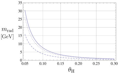
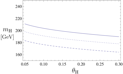
Figure 1: The masses of the radion and the Higgs boson as functions of $\theta_{\rm H}$. The solid, dotted, dashed lines represent the case of $\kappa=5.0,3.0,1.0$, respectively.

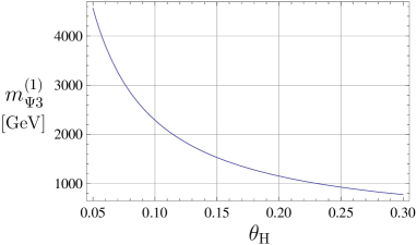
Figure 2: The mass of the first KK mode for $\Psi_{3}$ as a function of $\theta_{\rm H}$.

Now we show some numerical results. As a specific example, we consider the case of (3.4). Fig. 1 shows the radion and Higgs masses as functions of $\theta_{\rm H}$. The lightest KK mode comes from $\Psi_{3}$ when $\kappa<20$. Fig. 2 shows its mass as a function of $\theta_{\rm H}$. From these plots, we can read off the $\theta_{\rm H}$-dependence of each mass as

$$m_{\rm rad}\!\!\! \simeq\!\!\! \frac{\mbox{0.04 GeV}}{\sin^{2}\theta_{\rm H}},$$

$$m_{\rm H}\!\!\! \simeq\!\!\! \left(150-10\ln\sin\theta_{\rm H}\right)\mbox{ GeV},$$

$$m_{\Psi 3}^{(1)}\!\!\! \simeq\!\!\! \frac{k}{2e^{kL}}\simeq\frac{\mbox{230 GeV}}{\sin\theta_{\rm H}},$$ (4.15)

for $\kappa=1.0$. The radion-Higgs mixing angle is less than ${\cal O}(10^{-4})$ for $\sin\theta_{\rm H}\geq 0.06$. These results are consistent with the rough estimations (4.11) and (4.14).

Here we comment on the strength of the brane kinetic terms. We find that the modulus stabilization requires $\kappa\stackrel{{\scriptstyle>}}{{{}_{\sim}}}0.5$. For such values of $\kappa$, the Higgs mass is larger than 175 GeV at $\theta_{\rm H}=0.06$. Therefore, within the parameter space we consider, there is a region that is consistent with the latest excluded region 158 GeV$<m_{\rm H}<$175 GeV by the Tevatron [30]. Since the zero-modes for the gauge fields have (at least approximately) flat profiles, the 4D and 5D gauge couplings $g_{4}$ and $g_{5}$ are related through

$$\frac{1}{g_{4}^{2}}=\frac{L}{g_{5}^{2}}\left(1+\frac{\kappa}{kL}\right).$$ (4.16)

Thus the dominant contributions to $g_{4}$ come from the bulk terms and the brane kinetic terms only give small corrections for an ${\cal O}(1)$ value of $\kappa$. On the other hand, the brane kinetic terms with ${\cal O}(1)$ $\kappa$ affect the masses of the KK modes and their couplings to the zero-modes in a sizable way, and their impacts are discussed in Ref. [23, 29], for example.

4.3 Experimental constraints on the radion mass

Finally we comment on the experimental constraints on the radion mass. The couplings of the radion to other fields are obtained by expanding the 4D effective action in terms of $\tilde{\varphi}=r/\Lambda_{r}$, where $\Lambda_{r}=\sqrt{3M_{5}^{3}/(k(e^{2kL}-1))}\simeq\sqrt{6}e^{-kL}M_{\rm Pl}$. In the original Randall-Sundrum setup, in which all the standard model particles reside on the IR brane, they are expressed as [31, 32]

$${\cal L}_{\rm eff}\!\!\! =\!\!\! -\frac{1}{\Lambda_{r}}rT^{\mu}_{\;\;\mu}+\cdots,$$ (4.17)

where $T_{\mu\nu}$ is the energy-momentum tensor of the standard model. Namely, the radion couples to particles on the IR brane just like the standard model Higgs does with an extra factor $v/\Lambda_{r}$, where $v=246$ GeV. To particles propagating in the bulk, the radion couplings deviate from (4.17), but are of the same order of magnitude [33, 34]. Hence the radion couplings are very weak because $v/\Lambda_{r}=2.1\times 10^{-3}$ for our choice of the warp factor. Thus the radion mass is not constrained from the collider experiments. It can also be bounded from below by the consideration of the neutrino oscillation inside the supernova [38], but this lower bound is much lower than 1 GeV in our case.

In addition to the above tree-level couplings, the radion couplings to the photons and to the gluons also receive sizable one-loop contributions. These couplings are important for the production and the decay processes of the radion. They can be enhanced compared to the corresponding Higgs couplings  times $v/\Lambda_{r}$. (See, for example, Ref. [41].) However such enhancements are insufficient for compensating the suppression factor $v/\Lambda_{r}$, and for discovering the radion at the Large Hadron Collider.

The situation does not change so much even if a larger value of $e^{kL}$ is chosen. From the requirement that $M_{5}/k>4.5$ and $\sin\theta_{\rm H}<0.3$, the warp factor is bounded through (4.3) as $e^{kL}<2.3\times 10^{14}$ for an ${\cal O}(1)$ value of $\kappa$. Thus the suppression factor $v/\Lambda_{r}$ cannot be larger than 0.01, which is still too small to detect the radion at the colliders.

In the case that the fermion mass hierarchy is realized by the wavefunction localization in the extra dimension, the experimental bounds on the flavor-changing processes can provide stronger constraints on $m_{\rm rad}$ and $\Lambda_{r}$. According to the analysis of Ref. [35], they should satisfy $\Lambda_{r}m_{\rm rad}>2.3a_{ds}\mbox{ TeV}^{2}$, where $a_{ds}$ is a dimensionless constant that parameterizes the flavor violation and its typical values range between 0.03 and 0.12. Thus the most stringent bound on $m_{\rm rad}$ is that $m_{\rm rad}>2.7$ GeV for $e^{kL}=5\times 10^{13}$ and $m_{\rm rad}>10$ GeV for $e^{kL}=2.3\times 10^{14}$.

5 Summary

We have considered the modulus stabilization in the gauge-Higgs unification scenario, and estimate the radion and Higgs masses. Through the $\theta_{\rm H}$-dependences of $M_{5}$ and $g_{A}$ in (4.8), various mass eigenvalues depend on $\theta_{\rm H}$ nontrivially. We found that the masses of the radion, the Higgs boson and the KK modes all have different $\theta_{\rm H}$-dependences. In order to see them explicitly, we considered two classes of models which correspond to different extensions of the model in Ref. [14]. Qualitatively, we have the same results in both classes.

$$m_{\rm rad}\!\!\! \sim\!\!\! \sqrt{{\cal O}(20)}\times\frac{10^{-2}\mbox{ GeV}}{\sin^{2}\theta_{\rm H}},$$

$$m_{\rm H}\!\!\! \sim\!\!\! \sqrt{{\cal O}(3)}\times 90\mbox{ GeV},$$

$$m_{\rm KK}\!\!\! \sim\!\!\! \frac{{\cal O}(\mbox{500 GeV})}{\sin\theta_{\rm H}},$$ (5.1)

and the radion-Higgs mixing is negligible. As mentioned in our previous work [23], the boundary kinetic terms for the gauge fields are necessary for the modulus stabilization. An ${\cal O}(1)$ value of $\kappa$ in (2.2) is enough to stabilize the modulus. In contrast to the model in Ref. [14], the Higgs couplings to other particles do not deviate very much from the standard model values when $\theta_{\rm H}\ll 1$.

The radion couplings to the standard model particles are suppressed by factors of ${\cal O}(v/\Lambda_{r})$ compared to the corresponding Higgs couplings. Within the allowed region of the parameter space, such suppression factors are less than 0.01. Therefore collider experiments do not impose any constraints on $m_{\rm rad}$. However the experimental bounds on the flavor-changing processes can provide stronger bounds on $m_{\rm rad}$ if the fermion mass hierarchy stems from the wavefunction localization. Such bounds narrow the allowed range of $\theta_{\rm H}$ in some cases.

Cosmological impacts of the radion physics is an intriguing subject. For this direction, we might need to extend the works by Refs. [42, 43, 44] to deal with the one-loop effective potential at finite temperature in the Randall-Sundrum background. This is one of our future projects.

Acknowledgments

The author would like to thank N. Maru for discussions in the early stage of this work.

Appendix A Definitions of functions

Here we define functions that are useful to express $\rho^{I}(\lambda;\theta_{\rm H})$ in (2.8) and the effective potential. First we define the following functions from the Bessel functions.

$$F_{\alpha,\beta}^{\kappa}(\lambda)\!\!\! \equiv\!\!\! J_{\alpha}(\lambda)Y_{\beta}^{\kappa}(\lambda z_{L})-Y_{\alpha}(\lambda)J_{\beta}^{\kappa}(\lambda z_{L}),$$ (A.1)

where $z_{L}\equiv e^{kL}$, and

$$J_{\beta}^{\kappa}(u)\equiv J_{\beta}(u)-\kappa uJ_{\beta+1}(u),\;\;\;\;\;Y_{\beta}^{\kappa}(u)\equiv Y_{\beta}(u)-\kappa uY_{\beta+1}(u).$$ (A.2)

For calculations of the effective potential, we also define

$$\hat{F}_{\alpha,\beta}^{\kappa}(w)\equiv I_{\alpha}(w)K_{\beta}^{\kappa}(wz_{L})-e^{-i(\alpha-\beta)\pi}K_{\alpha}(w)I_{\beta}^{\kappa}(wz_{L}),$$ (A.3)

where

$$I_{\beta}^{\kappa}(u)\equiv I_{\beta}(u)+\kappa uI_{\beta+1}(u),\;\;\;\;\;K_{\beta}^{\kappa}(u)\equiv K_{\beta}(u)-\kappa uK_{\beta+1}(u).$$ (A.4)

Then the following relation holds.

$$F_{\alpha,\beta}^{\kappa}(iw)=-\frac{2}{\pi}e^{i(\alpha-\beta)\pi/2}\hat{F}_{\alpha,\beta}^{\kappa}(w).$$ (A.5)

The asymptotic behavior of $\hat{F}^{\kappa}_{\alpha,\beta}(w)$ for ${\rm Re}\,w\gg 1$ is

$$\hat{F}^{\kappa}_{\alpha,\beta}(w)=-\frac{e^{w(z_{L}-1)}}{2w\sqrt{z_{L}}}e^{i(\beta-\alpha)\pi}\left(1+\kappa wz_{L}\right)\left\{1+{\cal O}\left(w^{-1}\right)\right\}.$$ (A.6)

Appendix B Approximate form of effective potential

Here we show the approximate forms of (4.9). As mentioned in Ref. [22], the dominant contributions to the effective potential come from the gauge fields and the fermion fields with bulk masses that are close to $k/2$.

As an example, let us consider a sector whose mass spectrum is determined by

$$\rho^{I}(\lambda;\theta_{\rm H})=F_{\alpha-1,\alpha-1}^{\kappa}(\lambda)F_{\alpha,\alpha}^{0}(\lambda)-\frac{2\sin^{2}\theta_{\rm H}}{\pi^{2}\lambda^{2}e^{kL}}=0,$$ (B.1)

where $\alpha$ is close to one. In fact, $\alpha=1$ for the gauge sector, and $\alpha=M_{\Psi}/k+\frac{1}{2}$ for the fermion sector. Then, the integrand of (2.11) can be approximated for $\varphi\gg 1$ as

$$\ln\frac{\rho^{I}(iwe^{-\varphi};\theta_{\rm H})}{{\cal K}^{I}(we^{-\varphi}){\cal I}^{I}(w)}\!\!\! =\!\!\! \ln\frac{\rho^{I}(iwe^{-\varphi};0)}{{\cal K}^{I}(we^{-\varphi}){\cal I}^{I}(w)}+\ln\frac{\rho^{I}(iwe^{-\varphi};\theta_{\rm H})}{\rho^{I}(iwe^{-\varphi};0)}$$ (B.2)

$$=\!\!\! \ln\left\{1-\frac{I_{\alpha-1}(we^{-\varphi})K_{\alpha-1}^{\kappa}(w)}{K_{\alpha-1}(we^{-\kappa})I_{\alpha-1}^{\kappa}(w)}\right\}+\ln\left\{1-\frac{I_{\alpha}(we^{-\varphi})K_{\alpha}(w)}{K_{\alpha}(we^{-\varphi})I_{\alpha}(w)}\right\}$$

$$+\ln\left\{1+\frac{e^{\varphi}\sin^{2}\theta_{\rm H}}{2w^{2}\hat{F}_{\alpha-1,\alpha-1}^{\kappa}(we^{-\varphi})\hat{F}^{0}_{\alpha,\alpha}(we^{-\varphi})}\right\}$$

$$\simeq\!\!\! -\frac{I_{\alpha-1}(we^{-\varphi})}{K_{\alpha-1}(we^{-\varphi})}\frac{K_{\alpha-1}^{\kappa}(w)}{I_{\alpha-1}^{\kappa}(w)}+\frac{e^{\varphi}\sin^{2}\theta_{\rm H}}{2w^{2}\hat{F}_{\alpha-1,\alpha-1}^{\kappa}(we^{-\varphi})\hat{F}_{\alpha,\alpha}^{0}(we^{-\varphi})}$$

$$\simeq\!\!\! \begin{cases}\frac{2(we^{-\varphi}/2)^{2(\alpha-1)}}{\Gamma(\alpha-1)\Gamma(\alpha)}\left\{-\frac{K_{\alpha-1}^{\kappa}(w)}{I_{\alpha-1}^{\kappa}(w)}+\frac{\sin^{2}\theta_{\rm H}}{2wI_{\alpha-1}^{\kappa}(w)I_{\alpha}(w)}\right\},&(\alpha>1)\\ -\frac{1}{\ln(we^{-\varphi}/2)+\gamma}\left\{-\frac{K_{0}^{\kappa}(w)}{I_{0}^{\kappa}(w)}+\frac{\sin^{2}\theta_{\rm H}}{2wI_{0}^{\kappa}(w)I_{1}(w)}\right\},&(\alpha=1)\\ \frac{2\sin(\pi\alpha)}{\pi}\left\{-\frac{K_{\alpha-1}^{\kappa}(w)}{I_{\alpha-1}^{\kappa}(w)}+\frac{\sin^{2}\theta_{\rm H}}{2wI_{\alpha-1}^{\kappa}(w)I_{\alpha}(w)}\right\},&(\alpha<1)\end{cases}$$

where $kL$ in the definition of $\rho^{I}(\lambda;\theta_{\rm H})$ is replaced by $\varphi$, and $\Gamma(\alpha)$ is the Gamma function. We have used that $\left|\alpha-1\right|\ll 1$, and assumed that $w={\cal O}(1)$ because the above function exponentially decays for $w\gg 1$. Thus the contribution of this sector to $\hat{V}(\varphi,\theta_{\rm H})$ is negligible when $\alpha>1$. When $\alpha\leq 1$, it is estimated as

$$\hat{V}^{I}(\varphi,\theta_{\rm H})\!\!\! \equiv\!\!\! (-)^{2\eta_{I}}N_{I}\int_{0}^{\infty}\!\!dw\;w^{3}\ln\frac{\rho^{I}(iwe^{-\varphi};\theta_{\rm H})}{{\cal K}^{I}(we^{-\varphi}){\cal I}^{I}(w)}$$ (B.3)

$$\simeq\!\!\! \begin{cases}\frac{(-)^{2\eta_{I}}}{\varphi}\sum_{n=0}^{2}v_{n}^{I}\cos^{n}\theta_{\rm H},&(\alpha=1)\\ (-)^{2\eta_{I}}\frac{2\sin(\pi\alpha)}{\pi}\sum_{n=0}^{2}v_{n}^{I}\cos^{n}\theta_{\rm H},&(\alpha<1)\end{cases}$$

where

$$v_{0}^{I}\!\!\! =\!\!\! N_{I}\int_{0}^{\infty}\!\!dw\;w^{3}\left\{-\frac{K_{\alpha-1}^{\kappa}(w)}{I_{\alpha-1}^{\kappa}(w)}+\frac{1}{2wI_{\alpha-1}^{\kappa}(w)I_{\alpha}(w)}\right\},$$

$$v_{1}^{I}\!\!\! =\!\!\! 0,\;\;\;\;\;v_{2}^{I}=-N_{I}\int_{0}^{\infty}\!\!dw\;\frac{w^{2}}{2I_{\alpha-1}^{\kappa}(w)I_{\alpha}(w)}.$$ (B.4)

Here we have used that $\varphi\gg\left|\ln(w/2)+\gamma\right|$ in the integration region that gives dominant contributions. For $\kappa=1.0$ and $\alpha=1$, for example, $v_{0}^{I}\simeq 8.6$ and $v_{2}^{I}\simeq-5.4$. In general, we can see that $v_{0}^{I}={\cal O}(N_{I})$ and $v_{2}^{I}={\cal O}(-N_{I})$. For the gluon and photon sectors, in which $\rho^{I=G,\gamma}(\lambda;\theta_{\rm H})=\lambda F_{0,0}^{\kappa}(\lambda)$, the terms proportional to $\sin^{2}\theta_{\rm H}$ in (B.2) are absent. Thus we find that $v_{0}^{I}=-{\cal O}(N_{I})$ and $v_{1}^{I}=v_{2}^{I}=0$, where $N_{G}=24$ and $N_{\gamma}=3$.

For the $\Psi_{3}$-sector, in which $\rho^{I}(\lambda;\theta_{\rm H})$ is given by (3.3), we can estimate $\hat{V}^{I=\Psi_{3}}(\varphi,\theta_{\rm H})$ in a similar way and find that $v_{0}^{\Psi_{3}}={\cal O}(N_{\Psi_{3}})={\cal O}(24)$, $v_{1}^{\Psi_{3}}={\cal O}(-24)$ and $v_{n=2}^{\Psi_{3}}=0$.

As a result, we obtain

$$\hat{V}(\varphi,\theta_{\rm H})\!\!\! =\!\!\! \sum_{I}\hat{V}^{I}(\varphi,\theta_{\rm H})$$ (B.5)

$$\simeq\!\!\! -\frac{2\sin(\pi\alpha_{1})}{\pi}\left(v_{0}^{\Psi_{1}}+v_{2}^{\Psi_{1}}\cos^{2}\theta_{\rm H}\right)-\frac{2\sin(\pi\alpha_{3})}{\pi}\left(v_{0}^{\Psi_{3}}+v_{1}^{\Psi_{3}}\cos\theta_{\rm H}\right)$$

$$+\sum_{I=W,Z}\frac{1}{\varphi}\left(v_{0}^{I}+v_{2}^{I}\cos^{2}\theta_{\rm H}\right)+\sum_{I=G,\gamma}\frac{v_{0}^{I}}{\varphi}$$

$$=\!\!\! \sum_{n=0}^{2}\left(u_{n}+\frac{v_{n}}{\varphi}\right)\cos^{n}\theta_{\rm H},$$

where $u_{0}={\cal O}(-5)$, $u_{1}=u_{2}={\cal O}(3)$, $v_{0}=v_{2}={\cal O}(10)$ and $v_{1}=0$.

Appendix C Expressions for numerical calculations

Although the approximate expressions of the mass eigenvalues in (4.11) or (4.13) is useful for the order estimation of the mass eigenvalues, we need more accurate expression for the numerical calculation.

Here we consider the case of (3.4) as an example. Then, since the functions $\rho^{I}(\lambda;\theta_{\rm H})$ have the form of

$$\rho^{I}(\lambda;\theta_{\rm H})=\rho_{0}^{I}(\lambda)+\rho_{1}^{I}(\lambda)\cos\theta_{\rm H}+\rho_{2}^{I}(\lambda)\cos^{2}\theta_{\rm H},$$ (C.1)

we can expand the integrand of (2.11) around $\cos\theta_{\rm H}=c_{0}$ ($c_{0}$ is a constant) as

$$\ln\rho^{I}\!\!\! =\!\!\! \ln\left\{\rho_{0}^{I}+\rho_{1}^{I}c_{0}+\rho_{2}^{I}c_{0}^{2}\right\}-\sigma_{1}^{I}c_{0}+\sigma_{2}^{I}c_{0}^{2}$$ (C.2)

$$+\left(\sigma_{1}^{I}-2\sigma_{2}^{I}c_{0}\right)\cos\theta_{\rm H}+\sigma_{2}^{I}\cos^{2}\theta_{\rm H}+{\cal O}\left((\cos\theta_{\rm H}-c_{0})^{3}\right),$$

where

$$\sigma_{1}^{I}\equiv\frac{\rho_{1}^{I}+2\rho_{2}^{I}c_{0}}{\rho_{0}^{I}+\rho_{1}^{I}c_{0}+\rho_{2}^{I}c_{0}^{2}},\;\;\;\;\;\sigma_{2}^{I}\equiv\frac{2\rho_{0}^{I}\rho_{2}^{I}-\left(\rho_{1}^{I}\right)^{2}-2\rho_{1}^{I}\rho_{2}^{I}c_{0}-2\left(\rho_{2}^{I}\right)^{2}c_{0}^{2}}{2\left(\rho_{0}^{I}+\rho_{1}^{I}c_{0}+\rho_{2}^{I}c_{0}^{2}\right)^{2}}.$$ (C.3)

Thus $\hat{V}(\varphi,\theta_{\rm H})$ in (2.11) is expanded as

$$\hat{V}(\varphi,\theta_{\rm H})=\hat{V}_{0}(\varphi;c_{0})+\hat{V}_{1}(\varphi;c_{0})\cos\theta_{\rm H}+\hat{V}_{2}(\varphi;c_{0})\cos^{2}\theta_{\rm H}+{\cal O}\left((\cos\theta_{\rm H}-c_{0})^{3}\right),$$ (C.4)

where

$$\hat{V}_{0}(\varphi;c_{0})\!\!\! =\!\!\! \sum_{I}(-)^{2\eta_{I}}N_{I}\int_{0}^{\infty}\!\!dw\;w^{3}\left\{\ln\frac{\left(\rho_{0}^{I}+\rho_{1}^{I}c_{0}+\rho_{2}^{I}c_{0}^{2}\right)(iwe^{-\varphi})}{{\cal K}^{I}(we^{-\varphi}){\cal I}^{I}(w)}\right.$$

$$\left.\hskip 128.0374pt-\left(\sigma_{1}^{I}c_{0}-\sigma_{2}^{I}c_{0}^{2}\right)(iwe^{-\varphi})\right\},$$

$$\hat{V}_{1}(\varphi;c_{0})\!\!\! =\!\!\! \sum_{I}(-)^{2\eta_{I}}N_{I}\int_{0}^{\infty}\!\!dw\;w^{3}\left(\sigma_{1}^{I}-2\sigma_{2}^{I}c_{0}\right)(iwe^{-\varphi}),$$

$$\hat{V}_{2}(\varphi;c_{0})\!\!\! =\!\!\! \sum_{I}(-)^{2\eta_{I}}N_{I}\int_{0}^{\infty}\!\!dw\;w^{3}\sigma_{2}^{I}(iwe^{-\varphi}).$$ (C.5)

If we choose a constant $c_{0}$ as a solution to the equation,

$$c_{0}=-\frac{\hat{V}_{1}(kL;c_{0})}{\hat{V}_{2}(kL;c_{0})},$$ (C.6)

the correction term ${\cal O}((\cos\theta_{\rm H}-c_{0})^{3})$ in (C.4) can be neglected in the calculations of $m_{\rm rad}$ and $m_{\rm H}$.

References

- [1] D. B. Fairlie, Phys. Lett. B 82 (1979) 97; N. S. Manton, Nucl. Phys. B 158 (1979) 141.
- [2] Y. Hosotani, Phys. Lett. B 126 (1983) 309; Y. Hosotani, Annals Phys. 190 (1989) 233.
- [3] H. Hatanaka, T. Inami and C. S. Lim, Mod. Phys. Lett. A 13 (1998) 2601;
- [4] A. Pomarol and M. Quiros, Phys. Lett. B 438 (1998) 255.
- [5] I. Antoniadis, K. Benakli and M. Quiros, New J. Phys. 3 (2001) 20; G. von Gersdorff, N. Irges and M. Quiros, Nucl. Phys. B 635 (2002) 127; C. S. Lim, N. Maru and K. Hasegawa, J. Phys. Soc. Jap. 77 (2008) 074101; N. Maru and T. Yamashita, Nucl. Phys. B 754 (2006) 127; Y. Hosotani, N. Maru, K. Takenaga and T. Yamashita, Prog. Theor. Phys. 118 (2007) 1053.
- [6] C. Csaki, C. Grojean and H. Murayama, Phys. Rev. D 67 (2003) 085012; C. A. Scrucca, M. Serone and L. Silvestrini, Nucl. Phys. B 669 (2003) 128.
- [7] L. J. Hall, Y. Nomura and D. Tucker-Smith, Nucl. Phys. B 639 (2002) 307; L. J. Hall, H. Murayama and Y. Nomura, Nucl. Phys. B 645 (2002) 85.
- [8] L. Randall and R. Sundrum, Phys. Rev. Lett. 83 (1999) 3370.
- [9] Y. Hosotani and M. Mabe, Phys. Lett. B 615 (2005) 257.
- [10] K. Agashe, R. Contino and A. Pomarol, Nucl. Phys. B 719 (2005) 165.
- [11] R. Contino, L. Da Rold and A. Pomarol, Phys. Rev. D 75, 055014 (2007).
- [12] Y. Hosotani, S. Noda, Y. Sakamura and S. Shimasaki, Phys. Rev. D 73 (2006) 096006.
- [13] Y. Hosotani and Y. Sakamura, Phys. Lett. B 645 (2007) 442; Prog. Theor. Phys. 118 (2007) 935; Y. Sakamura, Phys. Rev. D 76 (2007) 065002.
- [14] Y. Hosotani, K. Oda, T. Ohnuma and Y. Sakamura, Phys. Rev. D 78, 096002 (2008) [Erratum-ibid. D 79, 079902 (2009)].
- [15] N. Haba, Y. Sakamura and T. Yamashita, JHEP 0907 (2009) 020; arXiv:0908.1042 [hep-ph].
- [16] Y. Hosotani, P. Ko and M. Tanaka, Phys. Lett. B 680 (2009) 179.
- [17] W. D. Goldberger and M. B. Wise, Phys. Rev. Lett. 83 (1999) 4922.
- [18] M. Fabinger and P. Horava, Nucl. Phys. B 580 (2000) 243.
- [19] J. Garriga, O. Pujolas and T. Tanaka, Nucl. Phys. B 605 (2001) 192; D. J. Toms, Phys. Lett. B 484 (2000) 149; W. D. Goldberger and I. Z. Rothstein, Phys. Lett. B 491 (2000) 339; I. H. Brevik, K. A. Milton, S. Nojiri and S. D. Odintsov, Nucl. Phys. B 599 (2001) 305.
- [20] R. Hofmann, P. Kanti and M. Pospelov, Phys. Rev. D 63 (2001) 124020.
- [21] E. Ponton and E. Poppitz, JHEP 0106 (2001) 019.
- [22] J. Garriga and A. Pomarol, Phys. Lett. B 560 (2003) 91.
- [23] N. Maru and Y. Sakamura, JHEP 1004, 100 (2010)
- [24] G. Cacciapaglia, C. Csaki and S. C. Park, JHEP 0603 (2006) 099.
- [25] A. D. Medina, N. R. Shah and C. E. M. Wagner, Phys. Rev. D 76 (2007) 095010.
- [26] H. Davoudiasl, J. L. Hewett and T. G. Rizzo, Phys. Lett. B 473, 43 (2000).
- [27] G. F. Giudice, R. Rattazzi and J. D. Wells, Nucl. Phys. B 595, 250 (2001).
- [28] C. Csaki, M. L. Graesser and G. D. Kribs, Phys. Rev. D 63, 065002 (2001).
- [29] H. Davoudiasl, J. L. Hewett and T. G. Rizzo, Phys. Rev. D 68 (2003) 045002 [arXiv:hep-ph/0212279].
- [30] [CDF and D0 Collaboration], arXiv:1007.4587 [hep-ex].
- [31] C. Csaki, M. Graesser, L. Randall and J. Terning, Phys. Rev. D 62, 045015 (2000).
- [32] W. D. Goldberger and M. B. Wise, Phys. Lett. B 475, 275 (2000).
- [33] T. G. Rizzo, JHEP 0206, 056 (2002).
- [34] C. Csaki, J. Hubisz and S. J. Lee, Phys. Rev. D 76, 125015 (2007).
- [35] A. Azatov, M. Toharia and L. Zhu, Phys. Rev. D 80, 031701 (2009).
- [36] R. Barate et al. [LEP Working Group for Higgs boson searches and ALEPH Collaboration and and], Phys. Lett. B 565, 61 (2003).
- [37] P. D. Acton et al. [OPAL Collaboration], Phys. Lett. B 268, 122 (1991).
- [38] U. Mahanta and S. Mohanty, Phys. Rev. D 62, 083003 (2000).
- [39] A. Falkowski, Phys. Rev. D 77, 055018 (2008).
- [40] N. Maru and N. Okada, Phys. Rev. D 77, 055010 (2008).
- [41] W. D. Goldberger, B. Grinstein and W. Skiba, Phys. Rev. Lett. 100, 111802 (2008).
- [42] P. Creminelli, A. Nicolis and R. Rattazzi, JHEP 0203, 051 (2002).
- [43] L. Randall and G. Servant, JHEP 0705, 054 (2007).
- [44] G. Nardini, M. Quiros and A. Wulzer, JHEP 0709 (2007) 077.