Jamming in complex networks with degree correlation.

Abstract

We study the effects of the degree-degree correlations on the pressure congestion $J$ when we apply a dynamical process on scale free complex networks using the gradient network approach. We find that the pressure congestion for disassortative (assortative) networks is lower (bigger) than the one for uncorrelated networks which allow us to affirm that disassortative networks enhance transport through them. This result agree with the fact that many real world transportation networks naturally evolve to this kind of correlation. We explain our results showing that for the disassortative case the clusters in the gradient network turn out to be as much elongated as possible, reducing the pressure congestion $J$ and observing the opposite behavior for the assortative case. Finally we apply our model to real world networks, and the results agree with our theoretical model.

I Introduction

It is known that a great variety of complex systems can be represented by networks, where the nodes are the elements of the system and the links, the interactions among them. A way to characterize a network is trough its degree distribution. In many cases of interest barabasi , this distribution is often scale free, which is characterized by a power-law degree distribution $P(k)\sim k^{-\lambda}$, ($k\geq k_{min}$), where $k$ is the number of connections that a node can have, $\lambda$ is the degree exponent and $k_{min}$ is the lowest degree allowed. The degree distribution has an important impact on the behavior of some dynamical processes taking place on the network, specially on the congestion problem Park ; Gulbahce ; NJP-us ; B-PRL ; PastorePRE ; LaRoccaPRE ; barabasi .

Recently the attention of scientists has been focused on to another characteristic of the complex networks: the degree correlation. The degree correlation can be understood as the tendency of nodes of a certain degree to be connected with other nodes with similar or different degree. In the first case this tendency is called assortativity and in the last one disassortativity.

Through this property, it is possible to separate social networks from technological networks, since the degree correlation behavior is very different in either case. In social networks, like the physics Co-authorship and film actors networks datasets , nodes tend to be attached with others of similar degree, and therefore are characterized by an assortative degree correlation. Technological and biological networks such as Internet and the protein-protein interaction instead have a disassortative degree correlation.

Despite there are several models of networks proposed in the literature that successfully reproduce many properties of real world networks, only recently a few of them, take into account the ”correlation” factor in their construction. Newman showed that models that do not consider correlation fail to reproduce many of the real networks properties Newman-r .

Of particular interest is to study the effects of the degree correlations on the dynamical processes evolving on the top of the network. It is known that some processes, such as synchronization Sorrentino , transport Xue , traffic dynamics Sun and growth Shao behave differently according to the correlations present in the substrate network where these processes spread Hu .

From a quantitative point of view, the degree correlation can be measured trough the neighbor connectivity Pastor-Satorras , introducing the quantity $K_{nn}(k)=\sum_{k^{\prime}}k^{\prime}P(k^{\prime}|k)$ where $P(k^{\prime}|k)$ is the conditional probability that an edge belonging to a node of degree $k$ points to a node of degree $k^{\prime}$. Then $K_{nn}(k)$ is the average nearest neighbor degree of a node of degree $k$. This function increases with $k$ in the case of an assortative network, decreases for a disassortative network and is flat for an uncorrelated network. Other measure of the degree correlation is the Pearson coefficient $r$ defined as

$$r=\frac{M^{-1}\sum_{e}j_{e}k_{e}-[M^{-1}\sum_{e}\frac{1}{2}(j_{e}+k_{e})]^{2}}{M^{-1}\sum_{e}\frac{1}{2}(j_{e}^{2}+k_{e}^{2})-[M^{-1}\sum_{e}\frac{1}{2}(j_{e}+k_{e})]^{2}}\;,$$ (1)

where $j_{e}$, $k_{e}$ are the degrees of the nodes at the ends of the $e$-th edge, with $e=1,...,M$, between $j_{e}$ and $k_{e}$. Notice that this expression is valid for undirected networks Newman03 . For assortative (disassortative) networks, $r>0$ ($r<0$), and $r=0$ for uncorrelated networks. Even though this is an accepted quantity to measure correlations, it should be used with caution because can hide strong structural correlations Dorogovtsev . Another measure of short range correlation is the clustering. The clustering coefficient $c_{i}$, for every site $i$ gives the probability that two nearest neighbors of node $i$ are also neighbor to each other.

Although there are many studies about degree correlations and clustering in the literature, there is no agreement among researchers on which topology characteristic governs a particular process that is evolving on the network. The problem is that the results obtained strongly depend on the algorithms used to build the correlated network, that in general generate clustering Newman ; Miller .

In our case, we are particularly interested in the effects of the degree correlations in the pressure congestion of a network. To this end we apply an algorithm that preserves the clustering and the degree distribution $P(k)$, but allows us to change the degree correlations. Then, through this algorithm we can isolate the effects of the degree correlations from clustering on the pressure congestion and compare the results with the uncorrelated case NJP-us . In particular we argue that real world networks of communications evolve to a disassortative form in order to enhance the transport trough them.

It is known NJP-us that for the uncorrelated case the pressure congestion increases with $\lambda$ when the process has a relaxational component. In NJP-us it was shown that by introducing a surface relaxation mechanism, congestion in SF networks can be reduced, but the same mechanism has no effect on congestion in the case of Erdös Renyi random graphs ER .

In order to study the effects of the degree correlations of the underlying network on the transport, we measure the congestion pressure $J$.

The congestion pressure of a network is measured in the gradient network. The gradient direction of a node $i$ is a directed edge pointing towards a neighbor $j$ on the substrate graph $G$, which has the lowest value of the scalar field of its neighborhood. If $i$ has the lowest value of $h$ in its network neighborhood, the gradient link is a self-loop. In other words, the gradient network is the collection of all gradient edges on the substrate graph $G$. In the gradient network, each node has just one outgoing link and $\ell$ incoming links. When a node has $\ell=0$, belongs to the perimeter of a gradient network cluster. Then $J$ is the average fraction of nodes with $\ell=0$, $J=N(\ell=0)/N$. Thus $J$ is a global indicator of the pressure congestion and higher $J$ means more congestion. In Ref. NJP-us the authors studied a dynamic process of gradient-induced flows produced by the local gradients of a non-degenerate scalar field ${\bf h}=h_{i=1}^{N}$ distributed over the $N$ nodes belonging to $G$. They found that the dynamic process decreases $J$ compared to the static case Znature . The findings in Ref. NJP-us were interpreted trough a structural transition in the clusters of the corresponding gradient networks.

Recently, Pan et al Pan studied the effects of the degree correlations on the pressure congestion in networks without any dynamics, using the model introduced in Gulbahce for the gradient network, and they found that assortative networks are less congested than disassortative. This founding contradicts the observation that most of the transport networks are disassortative. Transport in real networks cannot be thought as a static process.

Even though at the present time no one has a global understanding about what governs the evolution of complex networks, it is factual information that many of these networks have SF degree distribution. This include large-scale communication networks, and many biological networks. If there is a theory to explain this, it must be based on processes and principles that are common to all these different systems. So it is possible to think that the network structure and hence its evolution is tied to its main functionality, which is transport. However, transport is ubiquitously related to gradients, or biases distributed across the system. Therefore when a dynamic process is applied we expect a different behavior, that could explain why different kind of networks evolve with certain degree correlation.

In this paper we study the effect of the degree correlations on $J$ in SF networks when a dynamical process is applied.

II Theoretical Model

In this section we discuss the construction of the substrate networks with and without degree correlations used in this work. In order to generate uncorrelated SF networks we implement the configurational model ConfigModel , with a power law degree distribution, where the degree $k_{i}$ of a node $i$ is between $2=k_{min}\leq k_{i}\leq k_{max}=\sqrt{N}$ in order to uncorrelate the original network Boguna . Then, to correlate the original uncorrelated network, we apply the algorithm of rewiring links maslov ; xulvi1 ; xulvi2 , in which, at each step, two links of the network, connecting four different nodes are randomly chosen. Afterwards, the four nodes are ordered according to their degrees. If we want to correlate the network in a assortative mode, the links are rewired with probability $p$ in such a way that one link connects the two nodes with larger degrees and the other link connects the remaining nodes with smaller degrees and with probability $1-p$ the links are rewired at random. In the opposite case, if we want to correlate the network in a disassortative mode, with probability $p$, one link connects the highest degree node with the lowest degree node and the other link connects the remaining nodes. In both cases self-loops and multiple connections are forbidden. As can be seen the parameter $p$ controls the different degrees of assortativity or disassortativity that a network can have. Although we cannot achieve with this model the extremes value of $r$, to our end the values obtained are enough demonstrative since most of real world networks correlation fall in the range of values obtained by this model. We emphasize that this model does not change $P(k)$ and does not change clustering, which is very small in the original network.

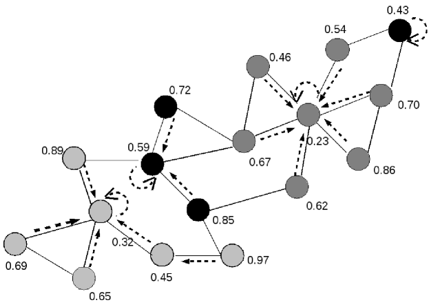
After building the SF network, at t=0, a random scalar field $h$ is constructed assigning to each node of the substrate network a random scalar uniformly distributed between $0$ and $1$. In Fig. 1 we show a scheme of the substrate network and the gradient network. Then the scalars $h\equiv h(t)$ evolve obeying the rules of the Family model Family ; note . This model is the simplest model of transport due to gradients, in which at every time step a node $i$ of the substrate is chosen at random with probability $1/N$ and it becomes a candidate for growth. If $h_{i}<h_{j}$ for every $j$ (gradient criterion) which is a nearest neighbor of the node $i$, $h_{i}\rightarrow h_{i}+1$. Otherwise, if $h_{i}$ is not a minimum, the node $j$ with minimum $h$ is incremented by one. When the process reaches the steady state of the evolution with this relaxation, we construct the gradient network and measure $J$ PastorePRE .

Figure 1: Scheme for the substrate network and the gradient network. The solid lines indicates the connections in the original network, that do not change during the process. The dash arrows indicate the connections in the gradient network and the self-loops. The numbers represent the scalar field of each node. Different colors represent different clusters in the gradient network. These clusters change as the dynamical process evolves. Notice that each cluster has just one self-loop.

III Results

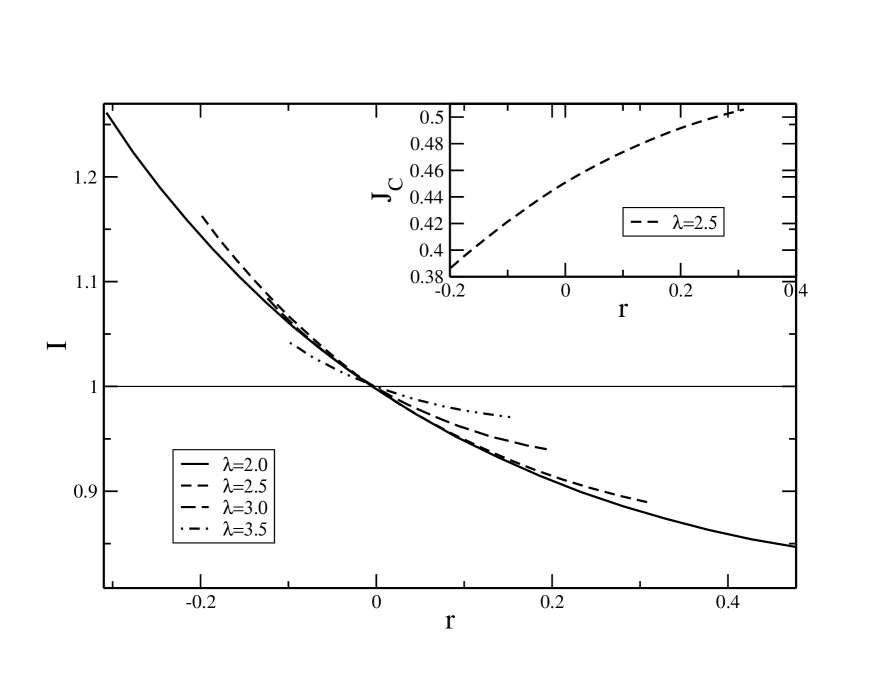
We run our simulations for SF networks with $k_{min}=2$ and $N=30000$. We choose this value of $N$ in order to avoid finite size effects on $r$ Dorogovtsev . We define $I=J_{U}/J_{C}$ as a factor of improvement, where $J_{U}$ is the pressure congestion for the uncorrelated network and $J_{C}$ for the correlated case. Then if $I>1$ ($I<1$) correlated networks enhance (worsen) the transport. In Fig. 2 we plot $I$ as function of $r$ for different values of $\lambda$. As can be seen in this figure, as $r$ decreases, $I$ increases, which means that a disassortative correlation leads, after dynamics, to a lower value of congestion, compared to an assortative correlation. This effect is more pronounced as $\lambda$ decreases, implying that disassortative networks are better for transport as $\lambda$ decreases. This result could explain the emergence of disassortative SF networks with small $\lambda$ in communication networks and agree with the idea that networks naturally develop certain correlation optimizing the process that evolves on the top of them. To give a general picture of $J_{C}$, in the inset of Fig.2 we plot $J_{C}$ as function of $r$ for $\lambda=2.5$. We can see that $J_{C}$ increases with $r$. This behavior was observed for different values of $\lambda$.

Figure 2: $I=J_{U}/J_{C}$ as function of $r$ for different values of $\lambda$ and $N=30000$. For $r<0$ the correlated structure has a lower jamming than the uncorrelated one. On the other hand, when $r>0$ the jamming is lower in the uncorrelated case. In the inset we plot $J_{C}$ as function of $r$ for $\lambda=2.5$. We can see that $J_{C}$ increases with $r$. We observe this behavior for different values of $\lambda$, not shown in this plot.

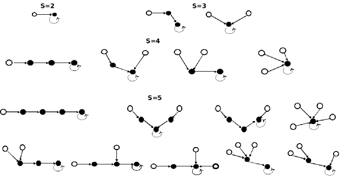
In order to understand the previous result, we are going to consider an ideal situation where a gradient network, in an infinite network, has every cluster configuration equally probable. For cluster configuration we mean every different way to connect the nodes of a cluster of size $s$ as it is shown in Fig. 3 for some values of cluster sizes. From Fig. 3 it can be seen that the average fraction of nodes in the perimeter of a cluster $\pi_{s}$ is almost constant as a function of $s$. More specifically, $\pi_{s}=1/2$ for $s=2,3,4$ and then decrease very slowly for larger sizes (for example, $\pi_{7}=0.482$). This implies that the average number of nodes in the perimeter of a gradient network cluster is a growing function of its size $s$. As a consequence, a gradient network with a large number of small clusters will have a smaller congestion pressure $J$ than a gradient network with a large number of big clusters. In a real network, the number and sizes of the gradient network clusters depends on the substrate network topology and on the relaxation process that evolves on the top of it. Let’s consider two archetype cases: first an assortative network where $N$ nodes are fully connected, i.e., every node has $N-1$ neighbors. The gradient network in this case is independent of the process and has just one cluster, with one self-loop and $N-1$ nodes in the perimeter. This example illustrate that when big clusters are present one have to expect a large number of nodes in the perimeter and a large jamming, which in this case is $J=N-1/N$ and tends to 1, i.e., maximum congestion. Second, a disassortative network with a star-like configuration, where one node is connected to the others $N-1$ nodes. In this particular case there will be more or less clusters in the gradient network depending on the efficacy of the process decongesting the network. For an optimal process we could obtain $N-2$ self-loops clusters (that means, clusters with $s=1$) and 1 cluster of size $s=2$. This example illustrate that when many small clusters are present one have to expect small number in the perimeter and a low jamming, which in this case is $J=1/N$ and tends to 0, i.e., minimum congestion. Extrapolating the conclusions given by this two toy networks, we expect smaller clusters and lower jamming for a disassortative networks comparison with an assortative one.

Figure 3: Clusters configurations for different cluster size $s$ (Here we show just from $s=2$ to $s=5$). The white nodes are the nodes in the perimeter ($\ell=0$) of every cluster. As can be seen there are a finite number of configurations for each size $s$ and as $s$ increases there are more possible configurations, but some of them have the same number of nodes in the perimeter. Notice that there is just one self-loop per cluster.

In the following, we are going to analyze what actually occurs with the process and the networks implemented in this work.

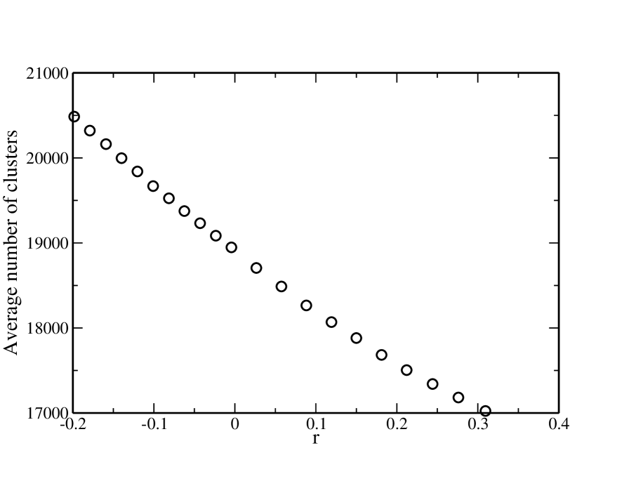
In Fig. 4 we plot the average number of clusters of the gradient network for different values of $r$ for our model. As can be seen, as $r$ decreases, there are more and consequently smaller clusters. Following our conclusions for an infinite gradient network the presence of smaller clusters indicates that a low number of nodes are in the perimeter of them and therefore it explains the lowering of the jamming observed in Fig. 2.

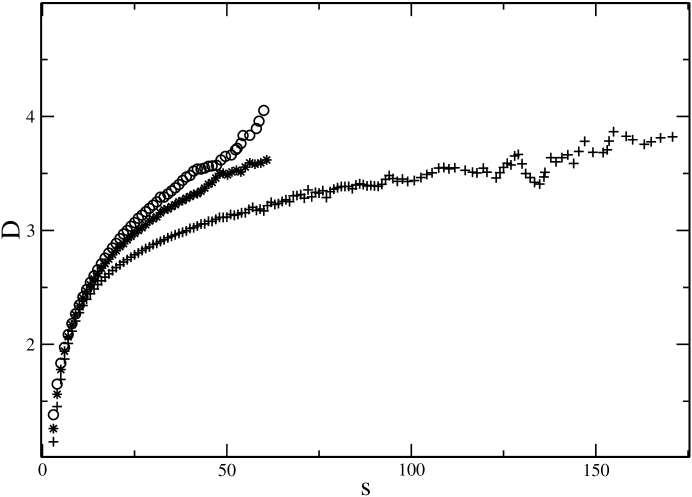
However, that conclusions were reached for infinite gradient networks of equally probable clusters. In order to observe the effect introduced by the network correlation and by the relaxation process favoring some specific graphs of Fig. 3 in detriment of others, in Fig. 5 we plot the average diameter $D(s)$ of the clusters as function of the cluster size $s$. We define $D(s)$ as the average distance from a perimeter node ($\ell=0$) to the self-loop of the cluster of size $s$ (see Fig.1). First, we observe that assortative networks reach a given diameter $D(s)$ for much bigger cluster sizes than disassortative networks. But bigger clusters with the same diameter is a clear indication that assortative networks have clusters with larger perimeters than disassortative ones, which confirms our previous conclusions based on infinite gradient networks. At the same time, we find that for a given cluster size $s$ dissortative networks show cluster with larger diameter than assortative ones. This is a new effect that cannot be inferred from our infinite gradient network analysis and is a consequence of the correlation in the substrate networks. The relaxation process running over them generate gradient network clusters that, for a given size $s$, are more elongated in the case of disassortative networks. More elongated clusters for a given size corresponds to a lower perimeter and hence to a lower congestion pressure $J$.

Figure 4: Average number of clusters decreases as $r$ increases for $\lambda=2.5$ and $N=30000$. This result was obtained for other values of $\lambda$ as well, observing the same behavior.

In order to see this effect in more detail, next we study the contribution of every cluster type (see Fig. 3) to the pressure congestion. Every cluster of size $s>1$ can have from $1$ to $s-1$ nodes in the perimeter, and of course this result does not depend on the correlation or the degree distribution of the network (See Fig. 3). What does depend on the degree correlation is the number of times that every configuration appears.

We observe that depending on the correlation of the substrate network, there are certain structures favored against others: for $r<0$ there are more self-loops clusters ($s=1$) than for $r>0$. We compute the number of clusters with $s=1$, for the values of $r$ in Table 1 before and after applying the relaxational process. We found that, in average, before the dynamics there are $3561.07$, $2.524$ and $1336.75$ self-loops clusters for $r=-0.198$, $r=-0.004$ and $r=0.309$ respectively. After the dynamics we find $7282.47$, $3960.96$ and $1391.51$ self-loops for the same values of $r$. This result means that disassortative correlations in combination with the relaxational process contribute to the decrease in the congestion. Something similar occurs for others values of $s$ showed in the Table 1. Besides from Table 1 for any value of $r$, for a given $s$ ($s=7$ as example) it can be seen that the cluster configurations with $1$ and $s-1$ nodes in the perimeter are less frequent than the others configurations. This result is due to there are different clusters configuration which lead to the same number of nodes in the perimeter, but for extreme cases ($1$ and $s-1$) there is only one possible configuration.

Figure 5: $D$ as function of $s$ for different values of $r$: disassortative ($\bigcirc$ $r=-0.198$), uncorrelated ($\ast$ $r=0.004$) and assortative ($+$ $r=0.309$), for $\lambda=2.5$ and $N=30000$.

From Table 1 we can also see that, after the dynamics, the pressure congestion has its main contribution from the smaller clusters. Computing the contribution to $J$ of the clusters from size $s=1$ to $s=7$ and we find that the nodes in the perimeter of these clusters represents more than the $75$% of the total perimeter for any value of $r$ in Table 1.

The results presented in this article do not depend on the algorithm used to build the substrate network (BA model or configurational model) neither the dynamical process , but some effects could be due to small features depending on the algorithm used to correlate the networks.

Finally, we want to show that our findings are reproducible in real-world networks. Here we present results for an Internet network dataNewman sample, the protein-protein interaction network of yeast, and the actor movie database datasets . We choose these networks because they are undirected and have a SF degree distribution: the Internet network has $r=-0.198$ and $\lambda=2.1$, the protein interaction network has $r=-0.156$ and $\lambda=2.4$, and the actors network has $r=0.208$ and $\lambda=2.3$ Havlin , so we have disassortative and assortative networks to compare with the uncorrelated case. In order to measure the pressure congestion in this real networks we assign a non degenerated scalar field to each node, and then we construct the gradient networks as it was explained previously in this paper, and perform the relaxation process. In order to compute the improvement factor $I$, we uncorrelate the real networks applying the following algorithm: at each step we choose two links connecting four different nodes and then we reconnect them at random avoiding self-loops and multiple connections. We found the following improvement factors $I_{Internet}=1.84\pm 0.02$ $I_{protein}=1.1\pm 0.02$ and $I_{actors}=0.86\pm 0.02$ which agree with our results found for model networks as function of the Pearson coefficient $r$ and the power-law exponent $\alpha$.

		1	2	3	4	5	6
	2	1538.29
		2909.09
$r=-0.198$	3	228.13	481.05
		759.39	624.12
	5	0.65	38.72	154.35	45.39
		13.12	195.73	237.28	1.17
	7	0.01	0.34	8.8	46.39	57.03	8.01
		0.13	8.75	60.06	87.93	31.07	0.74
	2	1979.30
		2925.49
$r=-0.004$	3	286.29	829.57
		666.95	961.39
	5	1.66	71.69	188.85	48.1
		14.39	249.5	250.96	20.11
	7	0.01	1.08	17.13	58.82	50.99	6.41
		0.14	13.64	79.80	97.14	28.28	0.8
	2	1879.64
		1932.18
$r=0.309$	3	326.62	1443.89
		426.59	1263.94
	5	4.29	170.1	271.22	59.48
		12.16	316.10	260.68	32.30
	7	0.01	5.94	44.32	83.14	81.43	4.45
		0.17	27.41	97.84	94.68	27.94	1.91

Table 1: For different values of $r$ we compute the number of every possible configuration, before and after (in italics) applying the dynamics, for different values of $s$ for $N=30000$ and $\lambda=2.5$. In this table we are only showing some values of $s$.

IV Conclusions

In the present work we studied the effects of the degree correlations to the congestion on SF complex networks when a dynamic process is applied. As a result we found that disassortative networks are better for transport compared to uncorrelated networks. This result could explain why real world networks of transport have $r<0$.

We also showed that the same relaxational dynamics has a bigger effect reducing the congestion in networks with lower values of $\lambda$. This result agree with the fact that real transportation networks evolve to structures with $2<\lambda<3$ and $r<0$.

We explained our results showing that for $r<0$ the clusters in the gradient network turn out to be as much elongated as possible, reducing the perimeter and hence the pressure congestion $J$ and observing the opposite behavior for $r>0$. We showed this computing the times that every cluster configuration appeared for some values of $s$.

Finally we applied our model to some real networks and the results show that these networks evolve to topologies that optimize certain processes.

References

- (1) R. Albert and A.-L. Barabási. Rev. Mod. Phys. 74, 47 (2002).
- (2) K. Park, Y-C Lai, L. Zhao and N. Ye, Phys. Rev E 71 065105(R) (2005).
- (3) N. Gulbahce, Chaos 17, 026105 (2007)
- (4) A. L. Pastore y Piontti, C. E. La Rocca, Z. Toroczkai, L. A. Braunstein, P. A. Macri and E. López, New Journal of Physics 10, 093007 (2008).
- (5) L. A. Braunstein, S. Buldyrev, R.Cohen, H. E. Stanley, Phys. Rev. Let. 91, 168701, (2003).
- (6) A. L. Pastore y Piontti, P. A. Macri and L. A. Braunstein, Phys. Rev E 76, 046117 (2007).
- (7) C. E. La Rocca, L. A. Braunstein and P. A. Macri, Phys. Rev E 77, 046120 (2008).
- (8) Data available at http://www.barabasilab.com
- (9) M. E. J. Newman, Phys. Rev. Let. 89 208701, (2002).
- (10) F. Sorrentino, M. di Bernardo, G. Huerta Cuéllar, S. Boccaletti, Physica D 224, 123-129, (2006).
- (11) Yu-hua Xue, Jian Wang, Liang Li, Daren He and Bambi Hu, Phys. Rev.E 81 037101, (2010)
- (12) J-T Sun, S-J Wang, Z-G Huang, Y-H Wang, Physica A 388, 3244-3248 (2009).
- (13) J. Shao, S.V. Buldyrev, L.A. Braunstein, S. Havlin and H.E. Stanley, Phys. Rev. E 80, 036105 (2009).
- (14) H-B. Hu and X-F. Wang, Europhysics Letter 86, 18003, (2009).
- (15) R. Pastor-Satorras, A. Vazquez, A. Vespignani, Phys. Rev. Lett. 87, 258701 (2001).
- (16) M. E. J. Newman, Phys. Rev.E 67 026126, (2003).
- (17) S. N. Dorogovtsev, A. L. Ferreira, A. V. Goltsev and J. F. F. Mendes, Phys. Rev.E 81 031135, (2010).
- (18) M. E. J. Newman, Phys. Rev. Let. 103 058701, (2009)
- (19) J. C. Miller, Phys. Rev. E 80, 020901 (2009).
- (20) B. Bollobás Random Graphs (Second Edition, Cambridge University Press) (2001).
- (21) Z. Toroczkai, K. E. Bassler, Nature 428, 716 (2004).
- (22) G-J Pan, X-Q Yan, W-C Ma, Y-H luo and Z-B Huang, Phys. Sc. 81 055804, (2010).
- (23) M. Molloy and B. Reed, Comb. Prob. and Comput. 6, 161 (1995).
- (24) M. Boguñá, R. Pastor-Satorras and A. Vespignani, Eur. Phys. J. B. 38, 205-209 (2004)
- (25) S. Maslov and K. Sneppen, Science 296, 910 (2002).
- (26) R. Xulvi-Bruner and I.M. Sokolov, Phys. Rev. E 70, 066102 (2004).
- (27) R. Xulvi-Bruner and I.M. Sokolov, Acta Physica Polonica B 36, 1431 (2005).
- (28) F. Family, J. Phys. A, 19, L441 (1986).
- (29) It is common to map this synchronization model into an interface growth model.
- (30) Snapshot of the structure of the Internet at the level of autonomous systems, reconstructed from BGP tables posted at archive.routeviews.org. This snapshot was created by Mark Newman from data for July 22, 2006.
- (31) R. Cohen, S. Havlin, Complex Networks: Structure,Stability and Function, Cambridge University Press, 2010.