The Balmer-dominated Bow Shock and Wind Nebula Structure of $\gamma$-ray Pulsar PSR J1741$-$2054

Abstract

We have detected an H$\alpha$ bow shock nebula around PSR J1741$-$2054, a pulsar discovered through its GeV $\gamma$-ray pulsations. The pulsar is only $\sim 1.5^{\prime\prime}$ behind the leading edge of the shock. Optical spectroscopy shows that the nebula is non-radiative, dominated by Balmer emission. The H$\alpha$ images and spectra suggest that the pulsar wind momentum is equatorially concentrated and implies a pulsar space velocity $\approx 150{\rm\,km\,s}^{-1}$, directed $15\pm 10^{\circ}$ out of the plane of the sky. The complex H$\alpha$ profile indicates that different portions of the post-shock flow dominate line emission as gas moves along the nebula and provide an opportunity to study the structure of this unusual slow non-radiative shock under a variety of conditions. CXO ACIS observations reveal an X-ray PWN within this nebula, with a compact $\sim 2.5^{\prime\prime}$ equatorial structure and a trail extending several arcmin behind. Together these data support a close ($\leq 0.5\;$kpc) distance, a spin geometry viewed edge-on and highly efficient $\gamma$-ray production for this unusual, energetic pulsar.

1. Introduction

PSR J1741$-$2054, discovered in a blind pulsation search of a Fermi point source (Abdo et al., 2009), is a $P=413$ ms, characteristic age $\tau_{c}=391$ kyr $\gamma$-ray pulsar. The pulsar was then detected in archival Parkes radio observations and subsequently studied at GBT (Camilo et al., 2009), showing it to be very faint and deeply scintillating. The radio observations also gave a remarkably low dispersion measure $DM=4.7\,{\rm pc\,cm^{-3}}$, which for a standard Galactic electron density model (Cordes & Lazio, 2002) implies a distance of $\approx 0.38$ kpc. This makes this one of the closest energetic pulsars known. At this distance the low flux density observed at pulsar discovery, $S_{1.4}\approx 160\mu$Jy, also makes this the least luminous radio pulsar known. Indeed, since the source scintillates to undetectability at many epochs, the time average radio luminosity is $L_{1.4}<0.025d^{2}_{0.4}{\rm\,mJy\,kpc}^{2}$. The low distance was already suspected from the relatively high $\gamma$-ray flux (for the modest ${\dot{E}}=9.4\times 10^{33}{\rm erg\,s^{-1}}$ spin-down luminosity). At the $DM$-estimated distance, the pulsar would emit 28% of its spin-down power in $\gamma$-rays, if the radiation were isotropic.

Since PSR J1741$-$2054 is an important addition to the set of nearby, energetic young pulsars, further investigation of its energy loss and environs are needed. In particular, we wish to constrain its motion, true age, non-photon spindown deposition and interaction with its environment. For example, it may be a significant source of $e^{\pm}$ injection in the solar neighborhood. Such injection is generally visible as a pulsar wind nebula (PWN). The shape of this nebula can constrain the source’s distance, ISM interaction, and proper motion. If the spin orientation can be measured (Ng & Romani, 2008), then we can also model the $\gamma$-ray beam shape and connect the observed $\gamma$-ray flux to its true luminosity, predicting $f_{\Omega}=L_{\gamma}/(4\pi F_{obs}D^{2})$ (Watters et al., 2009). This, in turn, provides the $\gamma$-ray efficiency, a critical test of pulsar models.

We accordingly searched for a PWN, discovering an H$\alpha$ bow shock and an X-ray PWN and trail. Like the few other pulsar bow shock nebulae, this is a non-radiative, Balmer-dominated shock. The shock velocity is relatively low, and Doppler broadened post-shock emission traces details of its flow, presenting an opportunity for the study of collisionless shock structure under unusual conditions, as well as constraining properties of the pulsar wind. We describe initial observations and conclusions here. Additional discussion of the X-ray PWN and of the spectral properties of the pulsar point source are presented in Sivakoff et al. (2011).

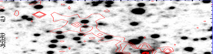
Figure 1.— WIYN 3.6m/MiniMo H$\alpha$ image of PSR J1741$-$2054’s bow shock. Contours show the CXO 0.7-7 keV emission, smoothed on a 14^′′ scale. Additional high contours smoothed at the 1^′′ scale mark the PSR/PWN core.

2. Observations

2.1. H$\alpha$ Imaging

Our initial detection of the PSR J1741$-$2054 PWN was made in a 600s exposure using the WIYN 3.6m telescope and the MiniMo camera with the KP W012 ($\lambda=6566\AA,\,\Delta\lambda_{FWHM}=16\AA$) narrow-band H$\alpha$ filter on March 24, 2009. An additional 4$\times 300$s exposure plus a continuum frame were obtained the next night. Unfortunately all data suffered from poor (1.4$-$1.8^′′) seeing. Nevertheless, these data revealed a clear elliptical ($13^{\prime\prime}\times 20^{\prime\prime}$) edge-brightened shell. As this is close to the Galactic bulge ($l=6.4^{\circ}\,b=4.9^{\circ}$), the continuum frame was crowded with field stars. Figure 1 shows the H$\alpha$ image, without continuum subtraction. We were able to use the spectroscopic flux calibration (see below) to estimate the total (continuum-subtracted) H$\alpha$ flux of the nebula as $F_{{\rm H}\alpha}\approx 1.5\times 10^{-14}{\rm erg\,cm^{-2}s^{-1}}$.

We subsequently (Aug 21, 2009) obtained 3$\times$600 s exposure using the EFOSC2 camera on the NTT 3.6m through the H$\alpha$#692 filter. While the image quality was somewhat better ($1.1^{\prime\prime}$), the wider ($\Delta\lambda_{FWHM}=62\AA$) transmission band and lower peak throughput gave the H$\alpha$ nebula sharper edge structure, but lower contrast (Figure 2). On this image we show the position of the CXO point source and the locations of the $1^{\prime\prime}$ slits used for the spectroscopic study.

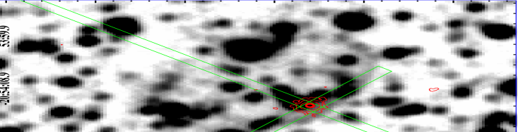
Figure 2.— NTT 3.6m/EFOSC2 H$\alpha$ image of the PSR J1741$-$2054 bow shock. Contours show the CXO 0.7-7 keV emission, smoothed on a 0.4^′′ scale. The two rectangular boxes show the 1^′′ wide long-slit positions of the Keck LRIS spectroscopy.

2.2. X-ray Imaging

We obtained a CXO/ACIS-S observation (ObsID 11251) of the pulsar field on May 21, 2010 (=MJD 55337.1), with 48.8 ks of exposure. The pulsar was placed near optimum focus on the backside illuminated S3 chip and the CCDs were operated in half-frame VFAINT mode, reading out every 1.64 s to reduce pileup. A bright point source and compact nebula are seen, locating the pulsar to 17h 41m 57.28s, $-$20^∘ 54^′ 11.8^′′ ($\pm 0.3^{\prime\prime}$). The crowded optical field made it difficult to identify field X-ray sources. However, over the S3 half-chip several soft (coronal emission) sources were clearly identified with field stars, confirming the X-ray/optical frame tie at the $\sim 0.3^{\prime\prime}$ level.

There is diffuse, faint X-ray emission in a PWN trail extending some $2^{\prime}$ at position angle PA=$45\pm 5^{\circ}$ (N through E). This structure contains $\sim 900\pm 100$ counts. From 2$-7^{\prime\prime}$ from the pulsar the trail contains an additional 92$\pm 14$ counts. Finally, the compact core contains $\sim 3460$ counts in a $2^{\prime\prime}$ radius region about the pulsar, dominated by the point source.

The emission from these structures is consistent with a simple absorbed power law with spectral index $\Gamma\approx 1.6\pm 0.2$ and absorbing column $N_{H}\approx 1.5\pm 0.3\times 10^{21}{\rm cm^{-2}}$. The point source clearly shows an additional soft thermal component, and the detailed spectral measurements of these structures are discussed in Sivakoff et al. (2011). Here we concentrate on the PWN morphology.

The region around the point source appears slightly extended. After subtracting a PSF generated with MARX, shifted and scaled to best match the point source component, the excess appears dominated by a diagonal band, $\approx 0.75^{\prime\prime}\times 2.5^{\prime\prime}$, with a minor axis at PA=$40\pm 5^{\circ}$. This structure appears to contain $\sim 400\pm 50$ counts or 11% of the total counts in this region. As the minor axis PA is within 5^∘ of the large scale X-ray trail axis (Figure 3), we associate this structure with the equatorial torus of the PWN. The 3:1 aspect ratio suggests a planar structure seen edge on, and implies that the pulsar spin axis is close to the plane of the sky.

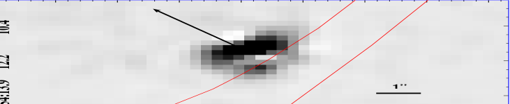
Figure 3.— PSF-subtracted PWN core, showing extended emission (excess in black). If interpreted as an equatorial torus, the symmetry axis lies within 5^∘ of the large scale trail axis (arrow) and the H$\alpha$ bow shock symmetry axis. The approximate location of the H$\alpha$ limb is shown by the curved band. X-ray photons ($0.7-7\;$keV) were binned to 0.25^′′ pixels and smoothed with a $\sigma=0.5^{\prime\prime}$ Gaussian after subtraction of a scaled MARX PSF.

2.3. Nebular Spectroscopy

Pulsar H$\alpha$ bow shock nebulae are relatively rare, since the pulsar wind must impact a partly neutral medium. Typically, this means that the pulsar has escaped its supernova remnant birthsite and is interacting with the general ISM (Chatterjee & Cordes, 2002). The shock spectra, however, are particularly interesting as the shocked gas is advected downstream on a time short compared to the cooling time. This means that these are non-radiative shocks and are dominated by Balmer emission rather than the usual forbidden lines (Raymond, 2001; Heng, 2010). When the up-stream neutral atoms, which are unaffected by the fields in the shock, drift into the shocked ISM gas they can be excited, producing line radiation at the (cold) radial velocity of the ambient medium gas. For typical conditions the ratio of excitation to ionization rates is $q_{ex}/q_{i}\approx 0.25$ so that we obtain an ISM-velocity Balmer photon for every $\sim 4$ neutral atoms. However, in addition, the atoms can charge-exchange with the hot shocked ions. This gives rise to excited neutrals in the post-shock flow and a broad line component at the systemic radial velocity of the post-shock gas. Thus spatially-resolved, kinematically-resolved observations of the line emission can provide a wealth of information on the local ISM and bow-shock kinematics (Aldcroft et al., 2002).

We were able to obtain two $1^{\prime\prime}$ long-slit spectra of the PSR J1741$-$2054 bow shock, using the Keck I/LRIS on June ll 2010 (MJD 55358.5). A total of 900s exposure was taken with the slit at ${\rm PA=}50^{\circ}$ (along the PWN symmetry axis) and 1200s total exposure with the slit at ${\rm PA=}140^{\circ}$. Both exposures covered the pulsar position. Unfortunately, since only one amplifier was available in the LRIS red camera, the long slit was truncated. However, we managed to cover the PWN emission; the slit locations were accurately determined from recorded slit images and are shown on Figure 2.

Figure 4.— Keck LRIS spectrum of the apex limb of the PSR J1741$-$2054 bow shock. The extreme Balmer dominance is evident, although the strongest forbidden lines are weakly detected from the bright patches on the limb.

For these observations, a 5600Å  dichroic separated the red and blue beams. The blue camera employed a 600l/mm, 4000Å  blaze grating and covered 3100-5600$\AA\,$ at a resolution of $\Delta\lambda=0.63\AA$/pixel. For the bow shock exposures, the red camera employed the 1200l/mm, 7500Å  grating for a resolution of $\Delta\lambda=0.4\AA$/pixel. With the 1^′′ slit the achieved resolution as measured from the night sky lines near H$\alpha$ was 1.48Å  or 68${\rm\,km\,s}^{-1}$ (FWHM). The spatial resolution along the slit was 0.24^′′/pixel. For the blue channel, we were able to employ standard calibrations. Unfortunately the red channel configuration was non-standard for the observing run and a flux standard was not obtained in this configuration. However, we were able to use flux measurements at a lower resolution setting along with measured grating responses to recover the red flux calibration with a conservative estimate of 15% accuracy. The wavelength calibration was refined by reference to the night sky lines and line velocities have been converted to the Local Standard of Rest (LSR) using the Mihalas & Binney (1981) constants.

Figure 4 shows the full spectrum of the bright limb in front of the pulsar from the $PA=50^{\circ}$ observation. The strong dominance of the Balmer emission is clear, although a few of the brightest forbidden lines are also visible. These lines were detectable only in the brightest portions of the shock limb, so we have not been able trace this component separately. Table 1 contains measurements of the line fluxes.

Table 1 PSR J1741$-$2054 Bow Shock Limb Fluxes

Species	Wavelenth	Flux
	$\AA$	$10^{-17}{\rm erg\,cm^{2}s^{-1}}$
H$\alpha$	6563	70.2$\pm 10.5$	a
H$\beta$	4861	17.6$\pm 0.5$
H$\gamma$	4340	5.2$\pm 0.6$
H$\delta$	4102	1.3$\pm 0.5$
N[II]	6583	4.0$\pm 0.7$	a
N[II]	6549	1.0$\pm 0.4$
O[I]	6300	1.6$\pm 0.3$
O[I]	6363	0.3$\pm 0.2$
O[II]	3727	4.8$\pm 0.5$
S[II]	6731	1.0$\pm 0.2$
S[II]	6716	1.2$\pm 0.3$

Our Balmer measurements give H$\alpha$/H$\beta=3.99\pm 0.61$ and H$\gamma$/H$\beta=0.295\pm 0.035$, and we can use these flux ratios to estimate the extinction toward the nebula. The selective extinction is

$$E(B-V)=2.21{\rm Log}({{\alpha/\beta}\over{\alpha/\beta_{m}}}),\,=-5.17{\rm Log}({{\gamma/\beta}\over{\gamma/\beta_{m}}})$$

where the models values (e.g. $\alpha/\beta_{m}$) depend on the shock populations and geometry, especially the shock optical depth of Ly$\beta$. Chevalier et al. (1980) have estimated the Balmer ratios for the broad component of a radiative shock (their Model 2). For the optically thin (Case A) situation, they find $\alpha/\beta_{m}=2.9$ and $\gamma/\beta_{m}=0.39$. Our corresponding extinction estimates are $E(B-V)=0.31\pm 0.15$ and $0.63\pm 0.26$; the $1\sigma$ overlap range is $E(B-V)=0.37-$0.46. However if the Ly$\beta$ optical depth is $\sim 3-5$, trapping increases the expected H$\alpha$ flux and the predicted broad line ratios are $\alpha/\beta_{m}=4.8$ and $\gamma/\beta_{m}=0.32$. The H$\alpha$ values then gives $E(B-V)<$0; physical, positive values are allowed only at the $\sim 1.3\sigma$ level. The H$\gamma$ flux gives $E(B-V)=0.18\pm 0.25$. Thus we conclude that the selective extinction is $<0.45$ with smaller values preferred for finite thickness shocks, especially for the H$\alpha$ measurement. For reference, the fitting formulae for extinction values in Chen et al. (1998) give $E(B-V)=A_{V}/3.1=0.13$ for this direction and $d=0.4\,$kpc. Our limit on the extinction can be translated to an effective Hydrogen column $N_{H}\approx 5.6\times 10^{21}E(B-V){\rm cm^{-2}}<2.5\times 10^{21}{\rm cm^{-2}}$, in agreement with the X-ray spectral fitting of the PWN. For either our conservative upper limit or the lower extinction inferred for modest optical depth shocks the neutral column is substantially larger than the low $N_{e}\approx 1.5\times 10^{19}{\rm cm^{-2}}$ inferred from the DM, suggesting low ionization along this line of sight.

With the spectral resolution and S/N available we were able to resolve the H$\alpha$ lines, making an initial exploration of the velocity structure in the post-shock flow. In Figure 5 we show the H$\alpha$ spectra along the two slit axes, with velocity shifts measured relative to the LSR as determined from night sky lines. Emission from the approaching (blue) and receding (red) sides of the bow shock are clearly seen in the PA=$50^{\circ}$ panel. Interestingly the front of the bow shock appears to be dominated by blue-shifted emission. We discuss a likely interpretation of this peculiar velocity structure below.

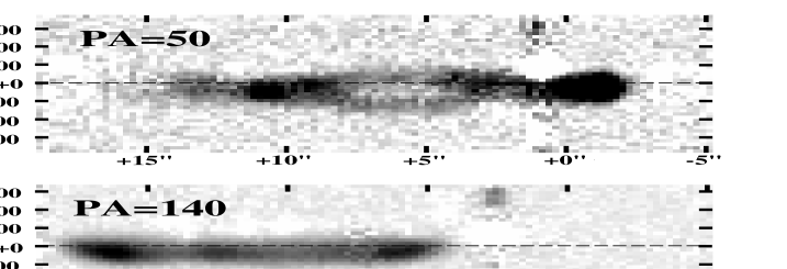
Figure 5.— Symmetry- (PA=$50^{\circ}$, above) and cross- (PA=140^∘, below) axis long slit spectra of the PSR J1741$-$2054 bow shock. Both pass through the estimated pulsar position at coordinate 0^′′. The spectra are sky- and continuum-subtracted and velocity shifts (${\rm km\,s^{-1}}$) are with respect to the LSR; residuals from bright stars appear, particularly 1.5^′′ behind the pulsar (PA=$50^{\circ}$) and 7^′′ to the right of the pulsar (PA=140^∘). The symmetry-axis spectrum shows red- and blue-shifted components from the front and back of the PWN shell. The cross-axis spectrum is dominated by blue-shifted emission near the front limb of the PWN.

3. Bow Shock Modeling

The spatial and kinematic information provided by these observations give an excellent opportunity to probe the geometry of the PWN outflow (Aldcroft et al., 2002). Very helpful in this study are the elegant solutions to the thin momentum-conserving bow shock provided by Wilkin (1996, 2000). Although these analytic results strictly only describe the shape of a contact discontinuity for a thin, fully mixed cold flow, they do provide a good approximate shape for the non-radiative forward shock in the ISM (Cormeron & Kaper, 1998; Bucciantini, 2002). The general velocity structure also follows the numerical simulations, although the cold analytic model has somewhat denser flows and correspondingly higher velocities downstream from the bow shock apex. The characteristic standoff angle of the contact discontinuity in the thin shock limit is

$$\theta_{0}=R_{0}/d=\left({{{\dot{m}_{W}}v_{w}}\over{4\pi\rho_{0}v_{\rm psr}^{2}}}\right)^{1/2}/d=2.1^{\prime\prime}{\dot{E}}_{34}/(n\,v_{7}^{2}\,d_{0.4})^{1/2}$$

where for a relativistic pulsar wind the momentum flux is ${\dot{m}_{W}}v_{w}={\dot{E}}/c$ and the numerical value is scaled to the nominal spindown flux and distance of PSR J1741$-$2054 traveling at 100$v_{7}{\rm\,km\,s}^{-1}$ through a medium of number density $n$. Thus we expect a small stand-off angle for the bow shock, as seen in Figure 1. Numerical simulations show that the forward ISM shock scale is a factor $\sim 1.3\times$ larger (Bucciantini & Bandiera, 2001).

However, Figure 1 shows that the observed H$\alpha$ shock is very flat at the apex; it does not fit well to the standard Wilkin (1996) thin shock solution. While the numerical thick bow shock models do show a somewhat wider angle spread downstream, they do not display the very small standoff and flattened apex of the PSR J1741$-$2054 bow shock. Effects that may produce such flattened structure are underlying wind asymmetry and projection to the Earth line-of-sight. Wilkin (2000) has provided useful expressions for the structure of anisotropic winds. In the pulsar case, we expect that the wind momentum flux will be axisymmetric about the pulsar spin axis. In general this provides momentum deposition misaligned with the bow shock axis. However, there is good evidence (Johnston et al., 2005; Ng & Romani, 2008) that pulsar spin and proper motion axis have a tendency to be aligned. We therefore focus on the aligned, axisymmetric wind.

The pulsar wind is also highly relativistic, so that the mass of the bow shock shell is dominated by the swept-up mass of the ISM. In the nomenclature of Wilkin (2000) this is $\alpha=v_{PSR}/v_{w}\longrightarrow 0$, while the aligned case is $\lambda=0$. We further restrict to an equatorially symmetric wind ($p_{w}=m_{w}v_{w}\propto c_{0}+c_{2}{\rm cos}^{2}\theta$). An isotropic wind has $c_{2}=0$ while an equatorial ($p_{w}\propto{\rm sin}^{2}\theta$) wind has $c_{2}=-3/2$. For these conditions the analytic solution is a surface of rotation with pulsar shock distance $R(\theta$) for $\theta$ the angle to the direction of the pulsar-ISM velocity with a cylindrical coordinate

$${\tilde{\bar{\omega}}}^{2}=(R/R_{0})^{2}{\rm sin}^{2}\theta=3(1-\theta\;{\rm cot}\theta)(1-c_{2}/12)+3c_{2}{\rm sin}^{2}\theta\;/4.$$

We can also write the tangential velocity (in the bow shock frame) and surface density of swept-up mass in the cold shell in terms of two quantities

$$G_{\tilde{\bar{\omega}}}=[(1-c_{2}/12)(2\theta-{\rm sin}2\theta)+{\rm sin}^{3}\theta\;{\rm cos}\theta]/4$$

and

$$G_{z}=[(1-c_{2}/12)(1-{\rm cos}2\theta)+c_{2}/2\,(2+{\rm cos}2\theta){\rm sin}^{2}\theta]/4$$

with

$$v_{t}=v_{PSR}[4G_{\tilde{\bar{\omega}}}^{2}+(2G_{z}-{\tilde{\bar{\omega}}}^{2})^{2}]^{1/2}/{\tilde{\bar{\omega}}}^{2}$$

the tangential surface velocity in the shell,

$$\sigma=n\;\mu m_{p}\;R_{0}({\tilde{\bar{\omega}}}^{2})^{1/2}v_{PSR}/(2v_{t})$$

the shell surface mass density, and $\mu m_{p}$ the mean mass per particle of the ambient ISM.

This bow shock structure will be axisymmetric in some angle $\phi$ about the pulsar velocity, which will be inclined by angle $i$ to the Earth line-of-sight. To complete the model of the bow shock appearance and radial velocity structure we project to the plane of the sky. This places the emission at projected angles $(\zeta,\chi)$ with respect to the (pulsar) wind origin with

$${\rm cos}\zeta={\rm cos}\theta\;{\rm cos}i+{\rm sin}\theta\;{\rm sin}i\;{\rm cos}\phi$$

and

$${\rm sin}\chi={\rm sin}\theta\;{\rm sin}\phi/{\rm sin}\zeta.$$

The emission from each point along the bow shock is proportional to the appropriate $\sigma(\theta,\phi)$ and the projected velocity (in the observer frame) is given by

$$v_{bs}=v_{t}({\rm cos}\gamma\;{\rm cos}i+{\rm sin}\gamma\;{\rm sin}i\;{\rm cos}\phi)-v_{\rm psr}\;{\rm cos}i$$

with $\gamma=\theta+{\rm tan}^{-1}[R/(dR/d\theta)]$.

Note that this velocity solution is for the mixed (cooled, zero pressure) flow of the swept up gas. In practice, numerical simulations show modest departures from this analytic solution for the tangential velocity (Bucciantini, 2002) and a detailed solution for the full line structure of the nebula should consider such effects. However, a more basic difference lies in the fact that the non-radiative H$\alpha$ arises from neutrals drifting into, and charge exchanging with, ions in the post-shock flow. Thus the H$\alpha$ structure depends strongly on the portion of this flow which is reached by such neutral atoms (Bucciantini & Bandiera, 2001). In particular, immediately behind the forward (ISM) shock we expect that the gas has velocity $3/4v_{\rm psr}{\rm cos}\eta$, where the angle between the pulsar velocity and the shock normal is $\eta=\theta-{\rm tan}^{-1}[(dR/d\theta)/R]$. Only later does the post-shock flow converge to the tangent to the contact discontinuity. This effect may be seen in the simulations of Cormeron & Kaper (1998). Thus immediately behind the ISM shock one expects a line-of-sight velocity

$$v_{nr}=-3/4v_{\rm psr}{\rm cos}\eta\;{\rm cos}i.$$

Since ${\rm cos}\eta$ is always positive, this velocity always has the sign of $-{\rm cos}i$.

3.1. Comparison with the Observations

An initial question is whether the shock created by an equatorial wind can reproduce the flattened shape of this pulsar bow shock. One way to parametrize this shape is the ratio of the perpendicular half angular size $\theta_{\perp}$, measured through the pulsar, to the angle from the pulsar to the projected limb of the wind shock in the forward direction $\theta_{||}$. Note that $\theta_{||}\neq\theta_{0}{\rm sin}i$. This ratio is very large for PSR J1741$-$2054’s bow shock, $\approx 3.7\pm 0.3$. We have computed this ratio for a number of axisymmetric, aligned wind bow shock models. Figure 6 shows that the projected shock limb has a ratio nearly independent of $i$ for an isotropic ($c_{2}=0$) wind, but that the ratio can reach the observed value for a ${\rm sin}^{2}\theta$ ($c_{2}=-3/2$) wind and a pulsar motion nearly in the plane of the sky. Considering winds that are even more equatorially concentrated or including the flaring effect of the finite pressure in a thick bow shock allows somewhat smaller $i$ to be accommodated.

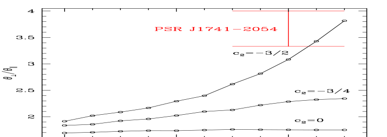
Figure 6.— Ratio of the perpendicular to standoff angular sizes as a function of $i$, the inclination angle of the pulsar velocity. The large ratio observed for PSR J1741$-$2054 is shown, suggesting an equatorially dominated wind and a pulsar velocity nearly in the plane of the sky.

Figure 7 shows the projected shape of an equatorial relativistic wind emanating from the pulsar position (circle) for an inclination $i=80^{\circ}$. For comparison, the line shows the limb of the isotropic wind bow shock; the standoff distance for the equatorial wind is appreciably reduced. Note that, since formally $p_{w}\propto{\rm sin}^{2}\theta$, the bow shock approaches the star in the forward ($\theta=0$) direction. Since the pulsar wind likely has a jet component, a physical bow shock would be smooth at the apex. Similar matching to the H$\alpha$ limb was used by Gaensler et al. (2002) to argue that the wind of the millisecond pulsar PSR J2124$-$3358 is anisotropic. For PSR J1741$-$2054 we have additionally been able to connect the shock shape with anisotropy detected in the X-ray synchrotron nebula (§2.2).

We next check if our model can explain the features of Figure 5. Most remarkable is the dominance of blue-shifted emission at and in front of the pulsar. For the PA=$50^{\circ}$ slit, the bright knot at the apex is at $v_{r}=-34$ to $-44{\rm\,km\,s}^{-1}$. The cross-axis slit has H$\alpha$ offset to $v_{r}=-29$ to $-44{\rm\,km\,s}^{-1}$, with no equivalent red-shifted component. This is significantly offset from the systemic (ISM) velocity. The lack of any red-shifted emission is at first surprising, given that mass flows around the bow shock. However, if the pulsar is moving out of the plane of the sky ($i<90^{\circ}$), we see that the prompt post-shock broad-line emission (from neutral atom charge exchange) will show negative radial velocities from both sides of the nebula. This is illustrated in the top two panels of Figure 8, which trace the velocity structure of the prompt emission. Here we plot a model for $i=70^{\circ}$ to better separate the velocity components. The $i=75-80^{\circ}$ models (for a 3D space velocity $v_{\rm psr}\approx 150\pm 50{\rm\,km\,s}^{-1}$) that match the shock shape also provide the best match to the velocity shifts in the slit spectra.

The immediate post-shock layers can dominate if the neutrals penetrate only partly into the shocked ISM, before suffering nearly complete ionization. This is equivalent to Case C of Bucciantini & Bandiera (2001). In fact PSR J1741$-$2054 has a relatively large spindown luminosity among pulsars showing ISM H$\alpha$ shocks (although below that of PSR B0740-28), so if the density and ionization fraction of the upstream medium are high, ionization may indeed be strong in the shocked ISM. Thus, ahead of the pulsar where the shock is nearly normal, neutral H may only exist in the immediate post-shock layer and blue shifted emission would dominate the observed spectrum.

The pulsar space velocity $v_{\rm psr}$ is modest and as one moves behind the pulsar position, the shock obliquity $\eta$ increases sharply and the post-shock heating drops. As ionization drops, neutral H may reach the bulk flow along the contact discontinuity (Bucciantini & Bandiera 2001 Case B). Charge exchange will continue and thus we expect components with negative radial velocity (near side) and positive radial velocity (far side). Indeed in Figure 5, across the body of the shell, the PA=$50^{\circ}$ spectrum shows two components with velocity extrema $-125{\rm\,km\,s}^{-1}$ and $+25{\rm\,km\,s}^{-1}$ from the front and back sides of the flow. Figure 8 shows the computed radial velocity for this ‘mixed component’. The large positive and negative velocities expected at the pulsar position are not seen in the PA=$140^{\circ}$ spectrum or in the PA=$50^{\circ}$ spectrum in front of the pulsar, suggesting that near the apex neutral H atoms do not penetrate to this ‘mixed’ tangential portion of the flow. The lower right panel shows a heuristic merged model, where the ‘mixed’ component grows as $\theta$ increases downstream. This smoothed model bears reasonable similarity to the observed 2D spectrum, although it fails to reproduce the ‘closed off’ shape along the symmetry axis and the red-shifted ‘mixed’ emission from the body of the nebula is less prominent in the data. Clearly additional effects are needed to reproduce the full velocity structure of this bow shock and additional imaging and spectroscopy will be needed to fully explain its origin. For example, the close-out of the symmetry axis spectrum suggests an expanding bubble structure rather than an open-backed bow shock. Bubble structure has been seen for other PWN bow shocks (e.g PSR B2224+65’s ‘guitar nebula’, Cordes et al. 1993); van Kerkwijk & Ingle (2008) have proposed that such bubble structures are a natural consequence of instabilities in the post-shock flow of the relativistic pulsar wind. The fainter and slower red wing ‘mixed’ emission 5-10^′′ behind the pulsar might be due to ISM inhomogeneities or, plausibly, instabilities in the PWN trail.

One additional difference to the data is the lack of an obvious ISM-velocity ‘narrow’ line component in the measured spectra. In the model spectra, the component is assigned 10% of the broad-line flux. The limited LRIS spectral resolution makes it difficult to discern any such component, particularly in the brighter knots of the bow shock emission. However, we estimate from the PA=$50^{\circ}$ spectrum of the nebular body a broad-to-narrow intensity ratio $I_{b}/I_{n}>3$. Interestingly, this ratio provides a measure of $T_{e}/T_{p}$, probing electron-ion equilibration in the post-shock emitting region (Raymond, 2001); relatively large ratios and fast equilibration appear to occur in low velocity shocks (van Adelsberg et al., 2008), supporting a modest velocity for PSR J1741$-$2054. If the narrow component can be isolated and kinematically resolved, it provides much additional information on the upstream medium’s density and on pre-shock heating of the ambient gas.

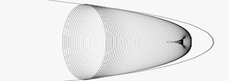
Figure 7.— Projected bow shock shape for an equatorial ($c_{2}=-3/2$) wind with pulsar velocity inclination $i=80^{\circ}$. The pulsar position is marked with a circle. Note that the projected bow shock limb has an appreciably flatter apex than that of an isotropic ($b_{3}=0$) edge-on ($i=90^{\circ}$) shock (line).

Figure 8.— Model slit spectra for an equatorial ($c_{2}=-3/2$) wind with pulsar velocity inclination $i=70^{\circ}$. The slit axes are at $10^{\circ}$ to the pulsar velocity vector and the pulsar position is marked (circle) at the systemic (narrow component) velocity. Above: prompt emission from the symmetry and cross axes. Below: The expected velocity structure of the ‘mixed’ gas emission for the PA=50^∘ slit, and a smoothed model where the mixed gas acquires a neutral component, appearing downstream.

4. Geometry and Distance Constraints

The leading edge of the bow shock appears structured, especially in the NTT image, so it is somewhat difficult to measure the pulsar-apex angle and cross-axis half angle. Our best estimates are $\theta_{||}\approx 1.5^{\prime\prime}$ and $\theta_{\perp}\approx 5.5^{\prime\prime}$. We would like to relate these to the characteristic contact discontinuity standoff angle $\theta_{0}$. In Aldcroft et al. (2002), the ISM shock/contact discontinuity angle ratio was estimated as $\sim 1.3$ at the shock apex. While finite pressure effects can cause this to grow slightly downstream, here we assume a constant ratio. Also, for the $c_{2}=-3/2$, $i=80^{\circ}$ shape, we infer $\theta_{||}=0.5\theta_{0}$ and $\theta_{\perp}=1.85\theta_{0}$. Together these estimates let us infer a characteristic (isotropic wind) contact discontinuity standoff angle $\theta_{0}\approx 2.3^{\prime\prime}$.

This characteristic offset implies $n\;d_{0.4}v_{7}^{2}=0.8$. As noted above the velocity structure suggests that $v_{7}\approx 1.5\pm 0.5$, so we loosely constrain the product $n\;d_{0.4}\approx 0.4$. In turn this suggests a plausible density $n\approx 0.4\;{\rm cm^{-3}}$ if we adopt the DM distance.

For the allowed extinction range ($A(H\alpha)=0-1.1$; i.e $\tau_{\rm Ly\beta}=0-5$), we infer an H$\alpha$ number flux from the full nebula of ${\dot{N}}_{\gamma}=5-15\times 10^{-3}{\rm cm^{-2}s^{-1}}$. This may be related to the neutral density and velocity of the upstream medium (Raymond, 2001; Ghavamian et al., 2001). For example the upstream neutrals will produce a narrow component H$\alpha$ number flux

$${\dot{N}}_{\gamma,n}\approx{{q_{ex}n_{HI}\pi(\theta_{eff}d)^{2}v}\over{q_{i}}4\pi d^{2}}=1.5\times 10^{-3}n_{HI}\theta_{10}^{2}v_{7}{\rm cm^{-2}s^{-1}}$$

for an excitation-to-ionization ratio $q_{ex}/q_{i}=0.25$ and effective full nebula angular radius $\theta_{eff}=10^{\prime\prime}\theta_{10}$. This predicts $\leq 0.3$ of the observed flux of the (broad) H$\alpha$ line. One can make a similar estimate for the flux of the broad component, depending on the ratio of charge-transfer to ionization rates, $q_{ct}/q_{i}$, i.e. $(q_{ct}/q_{i})n_{HI}\theta_{10}^{2}v_{7}=3-10$ (depending on the extinction). With the low $v_{7}\approx 1.5$ and $n\leq 1$ estimated above, we would infer a large yield of broad $H_{\alpha}$ photons from charge transfer interactions, $q_{ct}/q_{i}>2-7$. Figures in van Adelsberg et al. (2008) suggest that the broad to narrow ratio grows rapidly at low shock velocities, especially for optically thin shocks, although velocities as small as 150 ${\rm km\,s}^{-1}$ are not computed. Additional modeling and, especially, an accurate measurement of the narrow line component would help settle whether such high efficiency conversion to H$\alpha$ occurs.

Turning to the nebula distance, we see that the relatively low $N_{H}$ inferred from the X-ray absorption column and the Balmer line ratios supports a close distance for this pulsar, with the HI surveys (Dickey & Lockman, 1990; Kalberla et al., 2005) showing values twice that inferred for the nebula at distances as small as $0.5\;$kpc (HEASARC nH tool). With improved spectral measurements of the PWN H$\alpha$ we should be able to fit for a precise pulsar space velocity and inclination. Comparison with a proper motion, measurable from CXO X-ray imaging ($\sim$ 7y baseline) or possibly HST imaging (few year baseline) would then yield a direct kinematic distance to the neutron star. This is particularly valuable for understanding the apparently very high $\gamma$-ray efficiency.

Our match to the $\theta_{||}/\theta_{\perp}$ ratio suggests $i\approx 75\pm 10^{\circ}$. For our estimated $v_{p}\approx 150\,{\rm km\,s^{-1}}$ this is also consistent with the spread of velocities in our slit spectra and with the measured apex blue shift $\sim-30{\rm km\,s^{-1}}\approx(-3/4){\rm cos}(75^{\circ})150\,{\rm km\,s^{-1}}$ expected if the surrounding medium radial velocity is near the LSR and prompt emission dominates near the apex. If the pulsar spin and velocity are aligned, this implies a pulsar viewing angle $\zeta\geq 65^{\circ}$. In turn this may be compared with the viewing angles inferred for the observed $\gamma$-ray pulse profile (Romani & Watters, 2010). The two pole caustic (TPC) model has great difficulty producing the $\gamma$-ray pulse width $\Delta=0.23$ and lag from the radio $\delta=0.29$. In the outer gap (OG) picture, $\gamma$-rays for such an old pulsar are only seen if viewed from near the equator, $\zeta>60^{\circ}$, although the observed pulse width and $\gamma$-radio lag are then easily achieved. The best-fit prefers $\zeta\approx 65-75^{\circ}$, consistent with the angles inferred from the bow shock geometry above.

5. Conclusions

The discovery of an H$\alpha$ bow shock associated with the $\gamma$-ray pulsar PSR J1741$-$2054 provides an important opportunity to constrain the geometry and momentum deposition of a pulsar wind. Our initial images and spectra suggest that this pulsar wind has a strong equatorial concentration and that the spin axis (and space velocity) are close to the plane of the sky. The spectroscopy implies a low extinction (close distance) for the nebula, consistent with pulsar dispersion measure estimates. Spectra were obtained for two slices across the nebula which are best described by a pulsar velocity of $\sim 150{\rm\,km\,s}^{-1}$ directed $15\pm 10^{\circ}$ out of the plane of the sky. The variation in the spectrum along the nebula’s velocity axis suggests that different layers (prompt and then mixed) of the post-shock flow are emitting near the nebula apex and tail respectively. Some unmodeled features are seen and numerical simulation including pressure effects in the shock tail may be needed to explain the full velocity structure.

The apparently equatorially concentrated wind and near edge-on view are consistent with inferences of PWN flow from observations of other pulsars and with the $\gamma$-ray emission geometry inferred from LAT pulsations.

Pulsar H$\alpha$ bow shocks often display high symmetry suggesting that careful modeling can exploit their spatial and velocity structure to probe the dynamics of collisionless shocks in partly ionized media at a range of inclination angles. If, as suggested by our initial imaging and spectroscopy, the portion of the post shock flow probed by the H$\alpha$ emission varies along the bow shock surface, then the shock of PSR J1741$-$2054 provides an especially important laboratory to study the structure of collisionless non-radiative shocks. Improved measurements could precisely determine the anisotropy of the relativistic pulsar wind, may constrain the degree of wind-velocity alignment, and can help deliver a kinematic measurement of the pulsar distance. Such studies will, however, require higher spatial and spectral resolution data at good sensitivity. This might be acquired through intermediate resolution integral field studies or Fabry-Perot H$\alpha$ scans (Mann et al., 1999).

We thank Tony Readhead for collaboration on Fermi counterpart studies and for the LRIS integrations, and Aaron Meisner for help with the WIYN observing and MiniMo processing. We also thank Pablo Saz-Parkinson, Scott Ransom and Paul Ray for valuable discussions on the detection and distance of the LAT pulsars. Finally, we thank the referee, Marten van Kerkwijk, for a prompt, careful reading and useful suggestions that improved the text. This work was supported in part by NASA grants NNX08AW30G and NNX10AD11G and Chandra Grant GO0-11097X.

References

- Abdo et al. (2009) Abdo, A.A. et al. 2009, Science, 325, 840
- Aldcroft et al. (2002) Aldcroft, T.L., Romani, R.W. & Cordes, J.M. 2002, ApJ, 400, 638
- Bucciantini & Bandiera (2001) Bucciantini, N. & Bandiera, R. 2001, AA, 375, 1032
- Bucciantini (2002) Bucciantini, N. 2002, AA, 387, 1066
- Chen et al. (1998) Chen, B. et al. 1998, AA, 336, 137
- Camilo et al. (2009) Camilo, F. et al. 2009, ApJ, 705, 1
- Chatterjee & Cordes (2002) Chatterjee, S. & Cordes, J.M. 2002, ApJ, 575, 407
- Chevalier et al. (1980) Chevalier, R.A. et al. 1980, ApJ, 235, 186
- Cordes & Lazio (2002) Cordes, J.M. & Lazio, T.J.W. 2002, ArXiv:astro-ph/0207156
- Cordes et al. (1993) Cordes, J.M., Romani, R.W. & Lundgren, S.C. 193, Nature, 362, 133.
- Cormeron & Kaper (1998) Cormeron, F. & Kaper, L. 1998, AA, 338, 273
- Dickey & Lockman (1990) Dickey, J.M.. & Lockman, F.J. 1990, ARAA, 28, 15
- Gaensler et al. (2002) Gaensler, B. et al. 2002, ApJ, 580, L137
- Heng (2010) Heng, K. 2010, PASA, 27, 23
- Johnston et al. (2005) Johnston, S. et al. 2005, MNRAS, 364, 1397
- Kalberla et al. (2005) Kalberla, P.M. et al. 2005, AA, 440, 775
- Ghavamian et al. (2001) Ghavamian, P. et al. 2001, ApJ, 547, 995
- Mann et al. (1999) Mann, E.C., Romani, R.W. & Fruchter, A.S. 1999, AAS, 195, 4101
- Mihalas & Binney (1981) Mihalas, D. & Binney, J. ’Galactic Astronomy’
- Ng & Romani (2008) Ng, C.-Y., & Romani, R.W. 2008, ApJ, 673, 411
- Raymond (2001) Raymond, J.C. 2001, SpaSciRev, 99, 209
- Romani & Watters (2010) Romani, R.W. & Watters, K.P. 2010, ApJ, 714, 810
- Sivakoff et al. (2011) Sivakoff, G. et al. 2011, in prep
- van Adelsberg et al. (2008) van Adelsberg, M. et al. 2008, ApJ, 689, 1089
- van Kerkwijk & Ingle (2008) van Kerkwijk. M. & Ingle, A. 2008, ApJ, 683, 159
- Watters et al. (2009) Watters, K.P. et al. 2009, ApJ, 695, 1289
- Wilkin (1996) Wilkin, F.P. 1996, ApJ, 459, L31
- Wilkin (2000) Wilkin, F.P. 2000, ApJ, 532, 400