TUM-HEP-771/10

Characterising New Physics Models by
Effective Dimensionality of Parameter Space

Thorsten Feldmann, Christoph Promberger and Stefan Recksiegel

Physik Department, Technische Universität München, James-Franck-Straße,
D-85748 Garching, Germany

We show that the dimension of the geometric shape formed by the phenomenologically valid points inside a multi-dimensional parameter space can be used to characterise different new physics models and to define a quantitative measure for the distribution of the points. We explain a simple algorithm to determine the box-counting dimension from a given set of parameter points, and illustrate our method with examples from different models that have recently been studied with respect to precision flavour observables.

1 Introduction

With the LHC era having started, we are eagerly awaiting new particles or interactions to be detected at one of the dedicated high-$p_{T}$ experiments. Many of the alternative New Physics (NP) models under consideration introduce a set of additional parameters, notably in the flavour sector, where new sources for flavour transitions are introduced in the presence of additional fermionic or bosonic matter fields. The multi-dimensional parameter space of NP models is already constrained by phenomenological data: On the one hand, this implies exclusion limits, e.g. lower bounds on the masses of new particles. On the other hand, certain parameters or parameter combinations are less constrained, leaving room for more or less pronounced deviations from the Standard Model (SM). Depending on the particular NP models, the NP effects on different observables also show certain patterns of correlations, which can, for instance, be identified on the basis of a big sample of theoretically and phenomenologically allowed (but otherwise random) parameter points. The interplay between the results from direct production of new particles at the LHC and from the indirect constraints on flavour parameters in the quark and lepton sector will play a crucial role for establishing/excluding physics beyond the SM in the LHC era, see e.g. [1, 2, 3] and references therein.

In this paper, we will focus on the multi-dimensional parameter space of NP models and its interpretation, after the phenomenological constraints have been implemented in order to identify valid parameter points. A popular method to visualise correlations is to generate scatter plots for one observable or parameter against the other, on the basis of these points. The drawback of such a method is that only low-dimensional projections of parameter space can be studied. Moreover, the number or number density of points in certain regions of the scatter plots does not have an immediate statistical meaning. Below, we will advocate an alternative way to characterise the space of valid parameter points in a given NP model by its box-counting dimension (BCD): It takes into account the complete multi-dimensional structure of parameter space and is independent of the number of generated parameter points. In the next section we will first explain how the dimensionality of parameter space can be determined using the box-counting algorithm, which will be illustrated for some simple examples. Our method will then be applied to two explicit examples for NP models confronted with flavour phenomenology, and we will show how the BCD of parameter space can be used to classify different NP scenarios.

2 The box-counting algorithm

The BCD (or Minkowski dimension) of a set $S$ in a Euclidean space ${\cal R}^{n}$ is defined as

$$d={\rm dim}_{\rm box}(S)=\lim_{\epsilon\to 0}{\log N(\epsilon)\over\log 1/\epsilon}$$ (2.1)

where $N(\epsilon)$ is number of boxes of side length $\epsilon$ needed to cover $S$. For the cases that we consider, the BCD is equivalent to the Hausdorff dimension [4], which is frequently used to describe fractals.

In practise, we find the BCD by subdividing the parameter space into $(2^{i})^{n}$ boxes ($n$ is the dimension of the Euclidean space, i.e. the total number of parameters) and plotting the logarithm (base 2) of the fill ratio $f$ against $i$. For very small $i$, all boxes will be filled. For large $i$, if $(2^{i})^{n}\gg p$ (where $p$ is the number of valid points in parameter space that we found), no box will contain more than one point and the fill ratio will have a linear slope $-n$ in the logarithmic plot:

$$\log_{2}f(i+1)=\log_{2}{p\over(2^{i+1})^{n}}=\log_{2}{p\over(2^{i})^{n}}-n=\log_{2}f(i)-n$$ (2.2)

For intermediate values of $i$, the slope in the logarithmic plot gives us the dimension $d$ as $(d-n)$: From (2.1), with $\epsilon=1/2^{i}$ and $f(i)=N(1/2^{i})/(2^{i})^{n}$,

$$d={\log_{2}f(i)\cdot(2^{i})^{n}\over\log_{2}2^{i}}\quad\Rightarrow\quad\log_{2}f(i+1)-\log_{2}f(i)=d-n\,.$$ (2.3)

2.1 Example: The BCD of the coastline of Britain

The box counting algorithm can be used to show that the western coastline of Britain has a dimension of $d=1.25$[5].

Figure 1: The dimension of the coastline of Wales determined by box counting

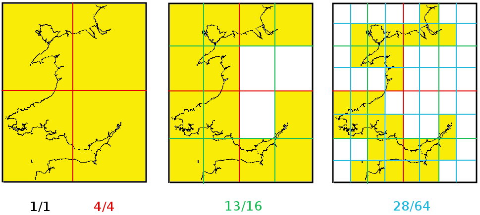
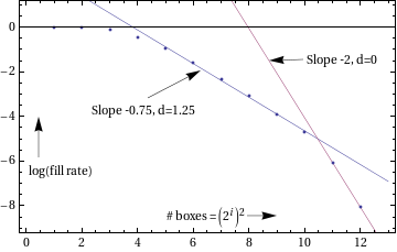
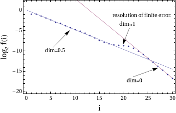
As shown in Fig. 1, the fill rate of successively smaller boxes will continually decrease. From the slope of the curve in the logarithmic plot, we can read off $d=2-0.75=1.25$, according to Eq. 2.3. For large $i$, the slope changes to $-2$, at this resolution we probe the single pixels of our image that have a dimension of $2-2=0$.

It is also possible to find an approximate self-consistency relation between the total number of pixels, $N_{\rm tot}$, the extracted BCD, $d$, and the iteration $i_{0}$ where the pixel resolution becomes too small and the kink in Fig. 1 occurs,

$$i_{0}\,d \simeq\log_{2}N_{\rm tot}\,.$$ (2.4)

For the above example, we started with $N_{\rm tot}=15600$ non-white pixels, which for $d=1.25$ corresponds to $i_{0}\simeq 11$. This is in perfect agreement with the kink position read off from Fig. 1.

2.2 Example: Solutions of $f(x)=\sin(1/x)$

For later discussion it is useful to consider another toy example, where we imagine that some physical observable $O$ depends on a fundamental theory parameter $x$ through

$$O(x) =\sin(1/x)\,.$$ (2.5)

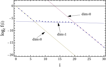
Having measured $O$ with some resolution $\Delta O$, we may ask for random points $x$ satisfying (2.5) within the uncertainties. Because of the non-trivial behaviour of $O(x)$, for a finite uncertainty $\Delta O$, the geometric shape of the resulting scatter plot (see Fig. 2) will correspond to a non-integer BCD.

Figure 2: Left hand side: Plot of $\sin 1/x$ indicating the range of $O(x)=0.5\pm\Delta O$ for $\Delta O=0.5\%$. Right hand side: Geometric shape of the corresponding solutions $\{x(O)\}$.

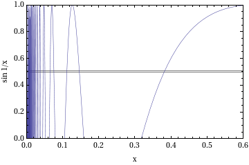
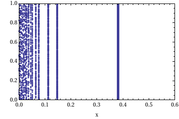
In Fig. 3 we show how the behaviour of $O(x)=\sin(1/x)$ differs from that of $\sin x$. While for $\sin(1/x)$ we observe the non-integer BCD, for $\sin x$ we first have $d=0$ (only one $x$ value reproduces the chosen $O(x)$), then $d=1$ (when we resolve the thickness of the chosen $\Delta O$, and then $d=0$ again (when we resolve the individual points).

Figure 3: Left hand side: Logarithm of the fill ratio for $O(x)=\sin 1/x$, Right hand side: Logarithm of the fill ratio for $O(x)=\sin x$.

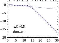
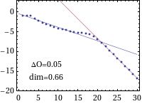
As expected, decreasing the uncertainty $\Delta O$ also leads to a decreasing BCD, and in the limit $\Delta O\to 0$, one finds some finite value corresponding to the dimensionality of the space formed by the set of solutions $\{x(O)\}$ in the considered interval for $x$, see (Fig. 4).

Figure 4: BCD for different values of $\Delta O$.

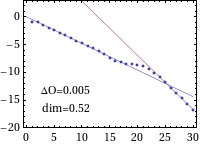
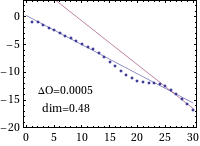
We would like to stress that in this toy model, we do not measure a fractal dimension since $\sin(1/x)$ is not self-similar. Still, for a given starting box, the BCD provides a useful quantitative measure of the distribution of the valid data points.

Let us for completeness compare this with the traditional measure for fine-tuning, derived from the normalised derivative [6],

$$\delta_{x}\equiv\left|\frac{x}{O(x)}\,\frac{dO(x)}{dx}\right| =\left|\frac{\cot(1/x)}{x}\right|\,,$$ (2.6)

which can be calculated for every valid parameter point $x(O\pm\Delta O)$. We find that the $\delta_{x}$ calculated in this way is different for each of the strips contributing to $\{x(O)\}$ and therefore not a good measure for the global distribution of points in this case, as we do not know how to form a meaningful average.

3 Application to New Physics Models

In this section we apply our method to two examples of new physics models, where the valid parameter space is described in terms of a set of points fulfilling the known constraints from flavour (and if applicable electroweak) observables.

3.1 A sequential fourth generation

One of the simplest extensions of the Standard Model (SM) is the addition of a sequential fourth generation (4G) of quarks and leptons [7] (for recent work, see e.g. [8, 9, 10, 11, 12, 13, 14, 15, 16]). We have studied this model extensively in [14], focusing on the phenomenological constraints and implications in the quark sector. We will use the parameter points generated for that paper in the subsequent analysis.

In the 4G quark sector, we have 10 parameters, of which 4 are SM parameters: The usual three mixing angles and the CKM phase. We perform two separate analyses of the 4G parameter space, either considering the space of all 10 parameters, or focusing only on the six new parameters. In both cases, we have to specify the multi-dimensional starting box, i.e. the lengths of the sides along the directions corresponding to the individual theoretical parameters. As a standard reference, we consider

$$\mbox{300~{}GeV}\leq m_{t^{\prime}}\leq\mbox{600~{}GeV}\,, 0\leq\theta_{ij}\leq\pi/2\,,\qquad 0\leq\delta_{ij}\leq 2\pi\,.$$ (3.7)

In this case, we find that – just as for the example of the coastline of Britain – there is a clearly defined linear region with a slope larger than $-n$ in the logarithmic plot of the fill rate, before the curve bends down to $-n$ for larger $i$.

Figure 5: Logarithmic plot of the fill rate for the 4G model, considering the 10-dimensional SM+NP parameter space. The steeper curve corresponds to a linear fit to the asymptotic behaviour ($i>6$), whereas the two other curves denote linear fits for $2\leq i\leq 5(6)$, with the slopes determining $d_{4G}-10$.

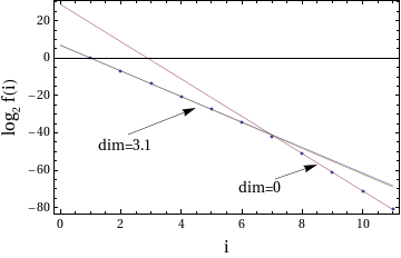
From the first linear region, we can read off a BCD of $d_{\rm 4G}=3.1$ with an uncertainty of approximately ${}\pm 0.1$.

This result is very stable: It does not depend on the number of generated points (which we varied between 5000 and $10^{6}$), and it also gives the same result, whether we include the SM parameters or not: Including the SM parameters for a total number of 10 parameters, the slope of the curve is approx. $-6.9$ (yielding the result $d_{\rm 4G}=3.1$ cited above). Analysing only the NP parameters, the number of parameters drops to 6, but the slope of the curve changes to $-3.0$, giving us the almost identical result of $d_{4G}=6.0-3.0=3.0$.

Figure 6: Logarithmic plot of the fill rate for the 4G model, considering only the 6-dimensional NP parameter space. The steeper curve corresponds to a linear fit to the asymptotic behaviour ($i>6$), whereas the two other curves denote linear fits for $2\leq i\leq 5(6)$, with the slopes determining $d_{4G}-6$.

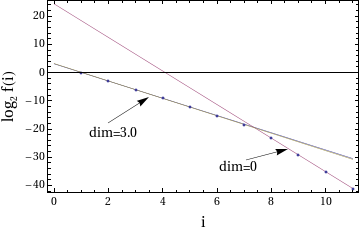
We stress here that the numerical result for the BCD depends on the size of the chosen starting box (cf. the toy example in Sec. 2.2). It can be seen that this indeed needs to be the case by considering the limiting cases of very small or very large boxes. Boxes smaller than the range of valid parameters are problematic for objects that are not completely self-similar (e.g. because of limited resolution: Looking only at the bay of Swansea will give a result different from that for the complete coastline of Wales). If, on the other hand, the box size is much larger in some dimension than the parameter range allowed for the corresponding parameter, the variation in that parameter cannot be resolved and will not contribute to the effective dimension of the parameter space (on a scale of $10^{9}$km, the coastline of Wales has no extent). In between these two extreme cases, we expect a residual logarithmic dependence on the size of the starting box.

Figure 7: Plot of the effective dimension against the logarithm of the box size for the parameter $\delta_{14}$. The three lines correspond to the fits for $1,2,3\leq i\leq 6$.

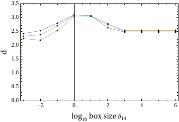
This is in fact the case as shown in Fig. 7 where the range for the 4G parameter $\delta_{14}$ is varied: For ranges from $10^{-3}$ to $10^{0}$, the granularity of our data points shows and the determined dimension is too small. Between $10^{0}=1$ and $10^{1}=10$ (where the natural value of $2\pi$ lies), we obtain our result of $\sim 2.9$, and between $10^{1}$ and $10^{3}$ we see the predicted fall-off. From $10^{3}$ on, the box is so large that the variation of $\delta_{14}$ cannot be resolved anymore and we obtain the dimension produced by the other parameters. At the same time we can see that the contribution of $\delta_{14}$ to the effective dimension of the whole parameter space is about $0.5$.

3.1.1 Ranking of individual 4G scenarios

As has been discussed in [14], the 4G parameter space can be divided into different regions which are characterised by the scaling of the 4G mixing angles with the Wolfenstein parameter $\lambda\simeq 0.22$,

$$\left(\theta_{14},\theta_{24},\theta_{34}\right) \sim\left(\lambda^{n_{1}},\lambda^{n_{2}},\lambda^{n_{3}}\right)\,.$$ (3.8)

Each triple of integers $(n_{1},n_{2},n_{3})$ then defines an individual 4G scenario. It has already been seen in [14] that different scenarios lead to rather different correlations, both between physical observables and between the new 4G CP phases.

We may ask ourselves whether this behaviour is also reflected in the BCD for the (now further restricted) parameter space within a given scenario $(n_{1},n_{2},n_{3})$. Indeed, we find that the dimension $d_{n_{1}n_{2}n_{3}}$ of individual scenarios is quite distinct. We can thus define a ranking between different scenarios according to the value of $d_{n_{1}n_{2}n_{3}}$. In Table 1, we show such a ranking for a selection of “interesting” scenarios which have been identified in [14].

Table 1: Ranking of some individual 4G scenarios according to their BCD.

Scenario ($n_{1},n_{2},n_{3}$)	Dimension $d_{n_{1}n_{2}n_{3}}$	# of Points
211	1.7	5486
221	1.7	5084
231	2.1	37k
432	2.2–2.4	29k
431	2.4–2.5	56k
332	2.5–2.6	125k
331	2.5	206k
321	2.6	295k

We have also quoted the number of points that have been found by the numerical procedure in [14] for the corresponding region of parameter space. Notice that the number or density of valid points does not necessarily allow for a quantitative or qualitative interpretation of the NP model under consideration, as it usually depends on the way the parameter points are generated (although in the shown case, the numerical procedure has treated all parameter values on equal footing, and therefore a smaller number of points also corresponds to a smaller BCD).

We observe that the scenarios 211 and 221 have the smallest dimension, with a value significantly below 2 and thus more than 1 unit lower than for the total valid parameter space. This is in line with the findings in [14], where these scenarios have been shown to give the most stringent constraints on the new 4G phases $\delta_{14}$ and $\delta_{24}$, and thus effectively reducing the dimensionality of the accessible parameter space by 1–2 units. (At the same time, these scenarios predict the most drastic and interesting deviations of flavour observables from their SM values.)

3.1.2 BCD of “forbidden” 4G scenarios

The 4G model provides a particular realisation of next-to-minimal flavour violation, according to the definition in [17]: It contains new sources of flavour and CP violation; still the new mixing angles are not expected to be generic but — as in the examples discussed in the previous subsection — naturally feature similar hierarchies as known from the 3G SM. Moreover, certain scenarios $(n_{1},n_{2},n_{3})$ can be (formally) excluded because of self-consistency inequalities among 3G and 4G mixing angles [17, 14],

$$\theta_{ik}\theta_{jk}\lesssim\theta_{ij}\qquad\mbox{(\small$i,j,k=1\ldots 4$, no summation over $k$).}$$ (3.9)

If these inequalities are violated, we expect a certain amount of fine-tuning between 4G parameters in order to keep the off-diagonal elements in the 4G mixing matrix sufficiently small.

Again, the BCD for such scenarios provides a measure to quantify this effect. In Table 2 we compare different scenarios that are classified by their minimal distance $\Delta^{2}=\sum_{i=1}^{3}\left(\Delta n_{i}\right)^{2}$ from one of the allowed scenarios (such that the allowed scenarios correspond to $\Delta^{2}=0$), For the forbidden scenarios, with increasing $\Delta^{2}$, we expect more and more fine-tuning and thus a smaller BCD $d_{\Delta}$. This is clearly confirmed by the numerical analysis which, for scenarios close to the allowed regions (i.e. $\Delta^{2}=1$) yields a BCD close to the one found from the allowed scenarios, whereas very distant scenarios yield BCDs which are more than one unit smaller.

Table 2: BCD of “allowed“ and “forbidden” 4G scenarios for different distance $\Delta^{2}$.

Scenarios ($n_{1},n_{2},n_{3}$)	Distance $\Delta^{2}$	Dimension $d_{\Delta}$	# of Points
(3,2,1), (3,2,2), (3,3,1), (3,3,2), …	0	2.60–2.80	166k
(3,4,1), (4,2,1), (5,3,1), (4,4,1), …	1	2.55–2.75	150k
(5,2,1), (6,3,2), (3,2,6), (2,1,5), …	2	1.9–2.0	7.8k
(6,3,1), (2,5,1), …	3	1.8–1.9	4.5k
rest	$\geq 5$	1.2–1.3	354

3.2 The Littlest Higgs Model with T parity

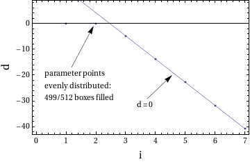
An elegant solution to the hierarchy problem are the Littlest Higgs Models [18, 19, 20, 21, 22] with $T$–parity (LHT) [23, 24, 25] which have been analysed in [26, 27, 28]. In this model, we encounter 9 new flavour parameters: Three mixing angles and three phases in the mixing matrix for the mirror quarks, and three mirror quark masses. The valid points in parameter space are distributed rather evenly over the available space: Of the $2^{9}=512$ boxes for $i=2$, 499 are filled (c.f. 8/1024 in the 4G case). For larger $i$, the fill rate quickly falls with $(2^{i})^{9}$ as expected for a dimensionless object. Unlike in the 4G model, we do not observe a kink corresponding to a non-trivial BCD, irrespective of the chosen starting values for the bounding box. In principle, this result allows for two different interpretations:

1. The dimensionality of the theoretical parameter space is indeed compatible with $d\simeq 0$. Indeed, this could have been anticipated from the results in [26, 27, 28], where these points have been characterised by the Barbieri–Giudice fine-tuning measure [6], cf. Eq. (2.6), yielding widely varying values up to and exceeding ${\cal O}(100)$.

2. Due to the limited number of generated valid parameter points for the LHT model (which, in turn, can be understood as a consequence of the required fine-tuning, respectively the small dimensionality of parameter space), the BCD measurement, in principle, allows for a second solution, when $N_{\rm tot}$ is too small to resolve the kink at $i_{0}\geq 2$ related to the “true” dimensionality. With (2.4) this can be easily translated to a bound on $d$,

   $$n\geq d \gtrsim\log_{2}N_{\rm tot}/2\,.$$ (3.10)

   In fact, for the LHT we only consider ${\cal O}(5k)$ points, and therefore, on the basis of the box-counting method alone, we cannot exclude BCDs between $6\lesssim d<9$. This means that the allowed points might lie on a structure that is too complex to be resolved with the number of points that we have at our disposal.

Figure 8: Logarithmic plot of the fill rate for the 9-parameter space of the LHT model.

4 Summary

We have proposed a novel method to study the distribution of parameter points in their multi-dimensional space. By employing a very simple box counting algorithm that can be applied to any data set, we obtain a measure for the effective number of free parameters and the amount of correlations induced by the phenomenological constraints. Unlike traditional measures of fine-tuning, the BCD method also works if the valid points have very different individual fine-tuning. Additionally, the BCD method uses only the valid data points and does not need to solve analytical expressions for the observables.

Using the well known example of the fractal dimension of coastlines and a toy model, it can be shown that the new measure makes sense even under variations of the box size and the number of points. The proposed method gives an easy and quick measure of the distribution of the points that would otherwise require many (necessarily low-dimensional) scatter plots to study.

The method is applied to two models of New Physics. For a sequential fourth generation of quarks, we show that the effective dimension of the parameter space is $\approx 3$, independent of whether the SM parameters are counted as variables or not (which is a highly non-trivial observation because of the complex dependence on the SM parameters). When classifying the points in 4G parameter space into different scaling scenarios, we find that the corresponding dimensions in parameter space are (i) smaller than those of the complete data set (ii) decrease with increasing distance from allowed scenarios.

Comparing the 4G findings with the phenomenologically valid points in the Littlest Higgs Model with T parity, we find that in the LHT model the effective dimension is 0 (corresponding to purely fine-tuned points) or very large (i.e. we do not have enough points to resolve the structure that they lie on).

Acknowledgements

We thank Björn Duling and Tillmann Heidsieck for helpful discussions. This research was partially supported by the Cluster of Excellence ‘Origin and Structure of the Universe’, the Graduiertenkolleg GRK 1054 of DFG and by the German ‘Bundesministerium für Bildung und Forschung’ under contract 05H09WOE.

References

- [1] F. del Aguila et. al., Collider aspects of flavour physics at high , Eur. Phys. J. C57 (2008) 183–308, [arXiv:0801.1800].
- [2] M. Artuso et. al., , and decays, Eur. Phys. J. C57 (2008) 309–492, [arXiv:0801.1833].
- [3] M. Raidal et. al., Flavour physics of leptons and dipole moments, Eur. Phys. J. C57 (2008) 13–182, [arXiv:0801.1826].
- [4] F. Hausdorff, Dimension und äußeres Maß, Mathematische Annalen 79 (1919), no. 1 157–179.
- [5] B. Mandelbrot, How Long Is the Coast of Britain? Statistical Self-Similarity and Fractional Dimension, Science 156 (1967), no. 3775 636–638.
- [6] R. Barbieri and G. F. Giudice, Upper Bounds on Supersymmetric Particle Masses, Nucl. Phys. B306 (1988) 63.
- [7] P. H. Frampton, P. Q. Hung, and M. Sher, Quarks and leptons beyond the third generation, Phys. Rept. 330 (2000) 263, [hep-ph/9903387].
- [8] W.-S. Hou, M. Nagashima, and A. Soddu, Enhanced from direct CP violation in with four generations, Phys. Rev. D72 (2005) 115007, [hep-ph/0508237].
- [9] W.-S. Hou, M. Nagashima, and A. Soddu, Large time-dependent CP violation in system and finite - mass difference in four generation standard model, Phys. Rev. D76 (2007) 016004, [hep-ph/0610385].
- [10] A. Soni, A. K. Alok, A. Giri, R. Mohanta, and S. Nandi, The Fourth family: A Natural explanation for the observed pattern of anomalies in CP asymmetries, Phys. Lett. B683 (2010) 302–305, [arXiv:0807.1971].
- [11] A. Soni, A. K. Alok, A. Giri, R. Mohanta, and S. Nandi, SM with four generations: Selected implications for rare and decays, Phys. Rev. D82 (2010) 033009, [arXiv:1002.0595].
- [12] M. Bobrowski, A. Lenz, J. Riedl, and J. Rohrwild, How much space is left for a new family of fermions?, Phys. Rev. D79 (2009) 113006, [arXiv:0902.4883].
- [13] O. Eberhardt, A. Lenz, and J. Rohrwild, Less space for a new family of fermions, arXiv:1005.3505.
- [14] A. J. Buras et. al., Patterns of Flavour Violation in the Presence of a Fourth Generation of Quarks and Leptons, arXiv:1002.2126.
- [15] A. J. Buras et. al., The Impact of a 4th Generation on Mixing and CP Violation in the Charm System, JHEP 07 (2010) 094, [arXiv:1004.4565].
- [16] A. J. Buras, B. Duling, T. Feldmann, T. Heidsieck, and C. Promberger, Lepton Flavour Violation in the Presence of a Fourth Generation of Quarks and Leptons, arXiv:1006.5356.
- [17] T. Feldmann and T. Mannel, Minimal Flavour Violation and Beyond, JHEP 02 (2007) 067, [hep-ph/0611095].
- [18] N. Arkani-Hamed, A. G. Cohen, and H. Georgi, (De)constructing dimensions, Phys. Rev. Lett. 86 (2001) 4757–4761, [hep-th/0104005].
- [19] N. Arkani-Hamed, A. G. Cohen, and H. Georgi, Electroweak symmetry breaking from dimensional deconstruction, Phys. Lett. B513 (2001) 232–240, [hep-ph/0105239].
- [20] M. Schmaltz and D. Tucker-Smith, Little Higgs Review, Ann. Rev. Nucl. Part. Sci. 55 (2005) 229–270, [hep-ph/0502182].
- [21] M. Perelstein, Little Higgs models and their phenomenology, Prog. Part. Nucl. Phys. 58 (2007) 247–291, [hep-ph/0512128].
- [22] N. Arkani-Hamed, A. G. Cohen, E. Katz, and A. E. Nelson, The littlest Higgs, JHEP 07 (2002) 034, [hep-ph/0206021].
- [23] H.-C. Cheng and I. Low, TeV symmetry and the little hierarchy problem, JHEP 09 (2003) 051, [hep-ph/0308199].
- [24] H.-C. Cheng and I. Low, Little hierarchy, little Higgses, and a little symmetry, JHEP 08 (2004) 061, [hep-ph/0405243].
- [25] I. Low, parity and the littlest Higgs, JHEP 10 (2004) 067, [hep-ph/0409025].
- [26] M. Blanke et. al., Particle antiparticle mixing, , , , , and in the littlest Higgs model with T-parity, JHEP 12 (2006) 003, [hep-ph/0605214].
- [27] M. Blanke et. al., Rare and CP-Violating and Decays in the Littlest Higgs Model with T-Parity, JHEP 01 (2007) 066, [hep-ph/0610298].
- [28] M. Blanke, A. J. Buras, B. Duling, S. Recksiegel, and C. Tarantino, FCNC Processes in the Littlest Higgs Model with T-Parity: a 2009 Look, arXiv:0906.5454.