General Scaled Support Vector Machines

Abstract

Support Vector Machines (SVMs) are popular tools for data mining tasks such as classification, regression, and density estimation. However, original SVM (C-SVM) only considers local information of data points on or over the margin. Therefore, C-SVM loses robustness. To solve this problem, one approach is to translate (i.e., to move without rotation or change of shape) the hyperplane according to the distribution of the entire data. But existing work can only be applied for 1-D case. In this paper, we propose a simple and efficient method called General Scaled SVM (GS-SVM) to extend the existing approach to multi-dimensional case. Our method translates the hyperplane according to the distribution of data projected on the normal vector of the hyperplane. Compared with C-SVM, GS-SVM has better performance on several data sets.

I Introduction

In past several decades, large margin machines have been widely studied and used. Support vector machines (SVMs) (also known as C-SVM) [1], the most important and effcient one proposed by Vapnik et al. [2], have been proven of good performance in text mining, bioinformatics, computer vision, and so forth [3, 4, 5]. Unlike many other classifiers minimizing the empirical risk, C-SVM is based on statistical learning theory [2], which emphasizes on minimizing the structural risk. C-SVM constructs a maximal margin between two classes. A hyperplane falls in the middle of this margin.

While the margin is solely determined by a few data points known as support vectors, remaining data points have no influence on building the classifier. Obviously, C-SVM loses some robustness because it cannot use the global information in the entire data set.

Inspired by this observation, we believe it is necessary to embed the global information into C-SVM. For a binary classification task, the distribution of two classes are usually not the same. It is reasonable to translate (i.e., to move without rotation or change of shape) the hyperplane closer to the class of the smaller variance. In [6], Feng proposed Scaled SVM (S-SVM) and gave a theoretical distance of the by extreme theory in 1-D case.

In this paper, we propose a simple method called General Scaled Support Vector Machine (GS-SVM) to generalize Feng’s method to multi-dimensional case. Our method has three steps. First, it uses C-SVM algorithms to obtain the hyperplane. Then it projects all data points onto the normal vector of the hyperplane and estimates the distribution of each class on this direction. Finally, it translates the hyperplane according to Feng’s conclusion. With kernel tricks, we can easily extend our method to feature space. In this framework, GS-SVM considers both local information of the data (SVs) and the global information.

The rest of the paper is organized as follows. In the next section, we give a brief background of C-SVM and Feng’s conclusion (S-SVM) that our method bases on. We extend 1-D S-SVM, to multi-dimensional case, GS-SVM, in Sect. III. Following that, we evaluate GS-SVM on toy data sets and several benchmarks. This paper is concluded in Sect. V.

II Background

II-A Support Vector Machines

Support Vector Machines are the implementations of Statistical Learning Theory [2] which emphasizes on minimizing structural risk. For a binary classfication problem, the two classes are labeled as $+1$ and $-1$ respectively. The C-SVM problem can be written as:

$$\begin{split}\min&\|\mathbf{w}\cdot\mathbf{w}\|+C\sum_{i=1}^{l}\xi_{i}^{2}\\ s.t.&\left\{\begin{array}[]{lc}y_{i}(\mathbf{w}\cdot\mathbf{x}_{i}+b)\geq 1-\xi_{i},\\ \xi_{i}\geq 0,\end{array}\right.i=1,2\ldots,l\end{split}$$ (1)

where $\xi_{i}\in\mathbb{R}$, $\mathbf{x}_{i}\in\mathbb{R}^{n}$ and $y_{i}\in\{+1,-1\}$ are the slack variable, feature vector and the label of the $i$-th data point respectively, $n\in\{1,2,\ldots\}$ is the dimension of feature vectors, $C$ is the penalty coefficient, and $l$ is the number of data points. To be solved, $\mathbf{w}\in\mathbb{R}^{n}$ (weighing vector) and $b$ (bias) determine the direction and offset of the hyperplane, respectively. $\frac{\|\mathbf{w}\cdot\mathbf{w}\|}{2}$ is known as the margin width. Laying in the middle of the margin, the hyperplane bears the equation $\mathbf{w}\cdot\mathbf{x}_{i}+b=\mathbf{0},\forall i\in 1..l$.

By the method of Lagrange multipliers, Eq. (1) is equivalent to:

$$\begin{split}\frac{\partial L}{\partial\mathbf{w}}&=\mathbf{w}-\sum_{i=1}^{l}y_{i}\mathbf{x}_{i}\alpha_{i}=\mathbf{0}\\ \frac{\partial L}{\partial\boldsymbol{\xi}}&=C\boldsymbol{\xi}-\boldsymbol{\alpha}=\mathbf{0}\\ \frac{\partial L}{\partial b}&=\sum_{i=1}^{l}\alpha_{i}y_{i}=0\\ \end{split}$$ (2)

where $L$ is the Lagrange function of Eq. (1), $\boldsymbol{\xi}=[\xi_{1},\xi_{2},\ldots,\xi_{l}]$, $\boldsymbol{\alpha}=[\alpha_{1},\alpha_{2},\ldots,\alpha_{l}]$ and $\alpha_{i}\geq 0$. Feature vector $x_{i}$ such that $\alpha_{i}\not=0$ is called a support vector.

Eq. (1) can be transformed into its dual form, which also allows the use of kernel tricks:

$$\begin{split}\max~{}&-\frac{1}{2}\boldsymbol{\alpha}^{T}\mathbf{Q}\boldsymbol{\alpha}\quad+\quad\frac{1}{2}\boldsymbol{1}^{T}\boldsymbol{\alpha}\\ s.t.~{}&\sum^{l}_{i=1}y_{i}\alpha_{i}=0\\ &\alpha_{i}\geq 0,i=1,\ldots,l\\ \end{split}$$ (3)

where $\mathbf{Q}$ is a matrix whose element at $i$-th row and $j$-th column is $Q_{ij}=y_{i}y_{j}\phi(\mathbf{x}_{i})\cdot\phi(\mathbf{x}_{j})$, and $\phi$ is a function, e.g., linear or radial basis, of the feature vector.

Figure 1: An illustration of Scaled-SVM in 1-D. $s_{1}$ and $s_{2}$ are the hyperplanes obtained by C-SVM and Scaled-SVM respectively.

II-B Scaled SVM

Due to the sparseness of $\boldsymbol{\alpha}$, the hyperplane is only related to a few points while other points have no influence. Therefore, C-SVM loses some robustness. Based on this observation, Feng [6] proposed Scaled SVM taking the distribution scale (range) of two classes into consideration. This method can advance C-SVM by at most $10\%$ on average generalization error.

Assume two classes $A_{1}$ and $A_{2}$ in one dimension are distributed in intervals $(0,a)$ and $(-b,0)$ respectively, where $a,b>0$. Let $s_{1}$ be the hyperplane obtained by C-SVM. Denote $d_{1}$ and $d_{2}$ as the distribution scales of $A_{1}$ and $A_{2}$, respectively. Let $c_{1}$ and $c_{2}$ be the distances from $s_{2}$ to the nearest points in $A_{1}$ and $A_{2}$, respectively. According to Scaled SVM, in parallel with $s_{1}$, the new hyperplane $s_{2}$ satisfies:

$$\frac{c_{1}}{c_{2}}=\sqrt{\frac{d_{1}}{d_{2}}}~{},$$ (4)

as illustrated in Fig. 1.

Eq. (4) can be reformulated into:

$$x_{new}=x_{old}+\Delta=x_{old}+\frac{2(\sqrt{d_{2}}-\sqrt{d_{1}})}{\sqrt{d_{1}}+\sqrt{d_{2}}}~{},$$ (5)

where $x_{old}$ and $x_{new}$ are the locations of $s_{1}$ and $s_{2}$ respectively. The calculation of $\Delta$ in multi-dimensional case will be determined later in the paper.

II-C Related Work

There have been many works which aim at combining the global information into C-SVM. Huang et al. proposed a new large margin classifier called Maxi-Min Margin Machine ($M^{4}$) which use the covariance information of two classes [7]. Yeung et al. first used clustering algorithms to determine the structure of data, then incorporated this structural information into constraints to calculate the largest margin [8]. In contrast to integrating global information into constraints, Xue et al. [9] proposed Structural Support Vector Machine, which embeds global information into the C-SVM’s objective function. This approach greatly reduces the computational complexity while keeping the sparsity merit of C-SVM. Xiong and Cherkassky proposed SVM/LDA which combined LDA and SVM together [10]. The SVM part reflects the local information of the data while the LDA part reflects the global information. Takuya and Shigeo improved the generalization ability of C-SVM by optimizing the bias term based on Bayesian theory [11].

III Our Proposed Method

III-A Overview

To a binary classification task, C-SVM will put the hyperplane in the middle of the margin. However, since the distributions of two classes are usually different, it makes sense to translate the hyperplane away from the class of larger variance and toward the other class. An illustration is shown in Fig. 2.

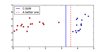
Figure 2: An illustration of our idea. The blue solid line is the hyperplane obtained by C-SVM. The red dash line is a better one for it is closer to the class (blue circles) with smaller variance on the horizontal direction.

Let the translating distance of the hyperplane be $\Delta$. The new SVM is the solution of the optimization problem below:

$$\begin{split}\min\quad&\|\mathbf{w}\cdot\mathbf{w}\|+C\sum_{i=1}^{l}\xi_{i}^{2}\\ s.t.\quad&\left\{\begin{array}[]{lc}y_{i}(\mathbf{w}\cdot\mathbf{x}_{i}+b)\geq 1+\Delta-\xi_{i},\text{~{}if~{}}y_{i}=+1\\ y_{j}(\mathbf{w}\cdot\mathbf{x}_{j}+b)\geq 1-\Delta-\xi_{j},\text{~{}if~{}}y_{j}=-1\\ \end{array}\right.\end{split}$$ (6)

Without losing of generalization, $i=1,2,\ldots,l^{+}$, $j=l^{+}+1,\ldots,l$, and $l^{+}$ is total number of positive class.

The solution of Eq. (6) is called a General Scaled SVM.

The Lagrange function of Eq. (6) is:

$$L = \frac{1}{2}\|\mathbf{w}\cdot\mathbf{w}\|+\frac{C}{2}\sum_{i=1}^{l}\xi_{i}^{2}$$

$$- \sum_{i=1}^{l^{+}}\alpha_{i}[y_{i}(\mathbf{w}\cdot\mathbf{x}_{i}+b)-1-\Delta+\xi_{i}]$$

$$- \sum_{j=l^{+}+1}^{l}\alpha_{j}[y_{j}(\mathbf{w}\cdot\mathbf{x}_{j}+b)-1+\Delta+\xi_{j}]$$

Eq. (6) is equivalent to

$$\begin{split}\frac{\partial L}{\partial\mathbf{w}}&=\mathbf{w}-\sum_{i=1}^{l}y_{i}\alpha_{i}\mathbf{x}_{i}+\frac{\partial\Delta}{\partial\mathbf{w}}\left[\sum_{i=1}^{l^{+}}\alpha_{i}-\sum_{j=l^{+}+1}^{l}\alpha_{j}\right]\\ &=\mathbf{w}-\sum_{i=1}^{l}y_{i}\alpha_{i}\mathbf{x}_{i}+\frac{\partial\Delta}{\partial\mathbf{w}}\sum_{i=1}^{l}\alpha_{i}y_{i}\\ &=\mathbf{w}-\sum_{i=1}^{l}y_{i}\alpha_{i}\mathbf{x}_{i}=\mathbf{0}\\ \frac{\partial L}{\partial\boldsymbol{\xi}}&=C\boldsymbol{\xi}-\boldsymbol{\alpha}=\mathbf{0}\\ \frac{\partial L}{\partial b}&=\sum_{i=1}^{l}\alpha_{i}y_{i}=0\\ \end{split}$$ (7)

Since Eq. (7) is identical to Eq. (2) (of C-SVM) and $L$ is independent from $\Delta$, this problem can be solved in three steps:

1. Use the C-SVM algorithm to obtain the original hyperplane.

2. Project all the points onto the normal vector of the hyperplane and estimate the distribution of each class in the projection.

3. Calculate $\Delta$ and translate the original hyperplane to obtain the new one.

Figure 3: An illustration of calculating $\Delta$.

III-B Calculating $\Delta$

After obtaining $\mathbf{w}$ from C-SVM training, we project data points onto the normal vector of the hyperplane. Then we utilize the projected scale of each class to adjust the hyperplane. This is illustrated in Fig. 3. Feng’s conclusion for 1-D SVMs can be extended to multi-dimensional case.

In the input space, the projected coordinate of any data point $\mathbf{x}_{i}$ on the normal vector of the hyperplane is:

$$e_{i}=\frac{\mathbf{w}\cdot\mathbf{x}_{i}}{\|\mathbf{w}\|}$$ (8)

Projected scales can be calculated as:

$$d_{1} = \max\mathbf{E}_{+}-\min\mathbf{E}_{+}$$

$$d_{2} = \max\mathbf{E}_{-}-\min\mathbf{E}_{-}$$

where $\mathbf{E}_{+}=\{e_{i}|y_{i}=+1\}$ and $\mathbf{E}_{-}=\{e_{i}|y_{i}=-1\}$.

With $d_{1}$ and $d_{2}$, $\Delta$ can be calculated as in Eq. (5):

$$\Delta=\frac{2(\sqrt{d_{2}}-\sqrt{d_{1}})}{\sqrt{d_{1}}+\sqrt{d_{2}}}$$

Note that $\Delta$ ranges from $-1$ to $1$.

In feature space, where all data points $\mathbf{x}$ are mapped into $\phi(\mathbf{x})$, since $\mathbf{w}=\sum_{i=1}^{l}\alpha_{i}\phi(\mathbf{x}_{i})$, all we need to do is replacing $\langle\mathbf{x}_{i}\cdot\mathbf{x}_{j}\rangle$ with $K(\mathbf{x}_{i},\mathbf{x}_{j})$.

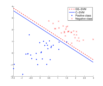
(a) training session

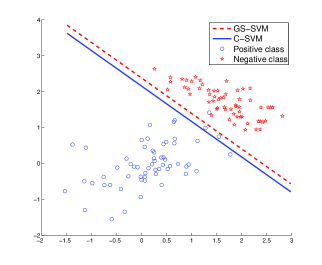
(b) testing session

Figure 4: An illustration of toy data.

IV Experiments

In this section, we first demonstrate the advantage of GS-SVM on synthetic 2-D toy data sets. Then we compare GS-SVM with C-SVM on several real world benchmarks. The training and testing of SVMs are accomplished by LIBSVM [12].

IV-A 2-D Toy Data

As illustrated in Fig. 4(a), the data set is generated under two Gaussian distributions: the positive class is randomly sampled from the Gaussian distribution with the mean as $[0.2,0.1]^{T}$ and the covariance as $[0.5,0.2;0.2,0.4]$, while the negative class is randomly sampled from another distribution with the mean and the covariance as $[1.7,1.7]^{T}$ and $[0.4,-0.2;-0.2,0.4]$. Training and test sets consist of 30 and 60 data points respectively for each class. Fig. 4(b) illustrates the hyperplanes derived by C-SVM and GS-SVM. From Fig. 4(b), we find that GS-SVM achieves a better hyperplane by taking both the local and global information of the data into consideration when determining the position of the hyperplane. As expected, the GS-SVM translates the hyperplane toward the class (negative class) of smaller projected scale on the normal of the hyperplane. GS-SVM classifies two more points correctly. The classification accuracies of C-SVM and GS-SVM are $96.67\%$ and $97.5\%$ respectively. The improvement on accuracy demonstrates the advantage of our proposed method.

IV-B Benchmarks

We also evaluate GS-SVM on 8 standard data sets from UCI machine learning repository [13]. GS-SVM are compared with C-SVM on both the linear and Gaussian kernels. The parameter $C$ for both methods is tuned via 10-fold cross validation. So is the width parameter of Gaussian kernel. The performance of these two methods in 10-fold cross validation is summarized in Table I.

data sets	linear kernel		Gaussian kernel
	C-SVM	GS-SVM	C-SVM	GS-SVM
sonar	73.72	75.10	88.47	89.87
liver	68.28	69.81	73.91	74.5
heart	83.33	83.71	83.33	84.44
spect	76.47	77.01	89.03	89.84
breast	96.81	96.81	97.22	97.36
statlog	84.95	84.95	86.37	86.95
diabet	76.95	77.34	77.86	78.26
hepatitis	78.28	80.39	83.28	84.54

TABLE I: Comparisons of classification accuracies among C-SVM and GS-SVM 

GS-SVM achieves a better performance on most data sets in both linear and Gaussian kernel. On remaining data sets, GS-SVM performs as well as C-SVM. The results on these benchmarks show that it is worth considering the global information of the data.

We notice an interesting role that $\Delta$ performs: GS-SVM can reach a higher accuracy with a smaller penalty value $C$ than C-SVM. It is not hard to understand from Eq. (6). We select “spect” data set as an example and show the relationship between $C$ and the accuracy in Fig. 5. Since the hyperplane translates toward the class of smaller projected scales on the normal of the hyperplane, it is more possible from the sum of slack variables $\sum_{i=1}^{l}\xi_{i}$ to decrease. $C$ is also used to minimize the classification error. The greater $C$ is, the smaller the classification error will be. As the hyperplane translates, it is more possible for classification error to drop. Hence, GS-SVM will achieve a better performance with a lower $C$. Note that although $C$ and $\Delta$ have the same effect of adjusting the position of the hyperplane, they do not work in the same way. $C$ adjusts the margin (the hyperplane lays in the middle of the margin) to minimize the training error, while $\Delta$ scales the position of the hyperplane to minimize structural risk.

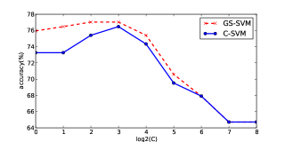
Figure 5: Accuracy versus C on “spect” data set.

V Conclusion

In this paper, we propose a simple but efficient method to improve the generalization ability of C-SVM, called as GS-SVM. C-SVM only uses support vectors and ignores the information of other data points. Previous works have been done to consider global information in deciding the hyperplane. For binary classification problem, one approach is to translate the hyperplane toward the class with smaller projected scale on the direction that is perpendicular to the hyperplane. However, existing work of this approach is only for 1-D case. In this paper, this approach is extended from 1-D to multi-dimensional cases. Experimental results show that GS-SVM advances C-SVM on both toy data sets and most of the benchmarks used. Throughout the paper, we discuss our method in the binary classification problem. However, it can be easily extended to multi-class classification problem. A future investigation will focus on theoretical analysis on the generalization ability of GS-SVM.

References

- [1] N. Cristianini and J. Shawe-Taylor, An Introduction to Support Vector Machines and Other Kernel-based Learning Methods, 1st ed. Cambridge University Press, 2000.
- [2] V. N. Vapnik, The Nature of Statistical Learning Theory. Springer-Verlag, 1995.
- [3] A. B. Goldberg, N. Fillmore, D. Andrzejewski, Z. Xu, B. Gibson, and X. Zhu, “May all your wishes come true: a study of wishes and how to recognize them,” in Proceedings of Human Language Technologies: The 2009 Annual Conference of the North American Chapter of the Association for Computational Linguistics, 2009, pp. 263–271.
- [4] W. S. Noble, “What is a support vector machine?” Nature Biotechnology, vol. 24, pp. 1565–1567, 2006.
- [5] K. Veropoulos, C. Campbell, and N. Cristianini, “Controlling the sensitivity of support vector machines,” in Proceedings of the International Joint Conference on AI, 1999, pp. 55–60.
- [6] J. Feng and P. Williams, “The generalization error of the symmetric and scaled support vector machines,” IEEE Transactions on Neural Networks, vol. 12, 1999.
- [7] K. Huang, H. Yang, I. King, and M. R. Lyu, “Learning large margin classifiers locally and globally,” in Proceedings of the Twenty-First International Conference on Machine Learning, 2004, p. 51.
- [8] D. Yeung, D. Wang, W. Ng, E. Tsang, and X. Wang, “Structured large margin machines: Sensitive to data distributions,” Machine Learning, vol. 68, pp. 171–200, 2007.
- [9] H. Xue, S. Chen, and Q. Yang, “Structural support vector machine,” in Proceedings of the 5th International Symposium on Neural Networks. Springer-Verlag, 2008, pp. 501–511.
- [10] T. Xiong and V. Cherkassky, “A combined SVM and LDA approach for classification,” in Proceedings of International Joint Conference on Neural Networks, 2005.
- [11] I. Takuya and A. Shigeo, “Improvement of generalization ability of multiclass support vector machines by introducing fuzzy logic and bayes theory,” Transactions of the Institute of Systems, Control and Information Engineers, vol. 15, pp. 643–651, 2002.
- [12] C.-C. Chang and C.-J. Lin, LIBSVM: a library for support vector machines, 2001, software available at http://www.csie.ntu.edu.tw/~cjlin/libsvm.
- [13] A. Frank and A. Asuncion, “UCI machine learning repository,” 2010. [Online]. Available: http://archive.ics.uci.edu/ml