Higher-order coupled quintessence

Abstract

We study a coupled quintessence model in which the interaction with the dark matter sector is a function of the quintessence potential. Such a coupling can arise from a field dependent mass term for the dark matter field. The dynamical analysis of a standard quintessence potential coupled with the interaction explored here shows that the system possesses a late time accelerated attractor. In light of these results, we perform a fit to the most recent Supernovae Ia, Cosmic Microwave Background and Baryon Acoustic Oscillation data sets. Constraints arising from weak equivalence principle violation arguments are also discussed.

I Introduction

Cosmological probes indicate that the universe we observe today possesses a flat geometry and a mass energy density made of $\sim∼30\%$ baryonic plus cold dark matter and $70\%$ dark energy, responsible for the late-time accelerated expansion. Unveiling the origin and the nature of dark energy is one of the great challenges in theoretical cosmology. The simplest candidate for dark energy is the cosmological constant, which corresponds to a perfect fluid with an equation of state $w=p/\rho=-1$. The $\Lambda$CDM model, i.e. a flat universe with a cosmological constant, is in very good agreement with current observational data. However, from the quantum field approach, the bare prediction for the current vacuum energy density is $\sim 120$ orders of magnitude larger than the measured value. This situation is the so-called cosmological constant problem. In addition, there is no proposal which explains naturally why the matter and the vacuum energy densities give similar contributions to the universe’s energy budget at this moment in the cosmic history. This is the so-called why now problem. A possible way to alleviate this problem is to assume a time varying, dynamical fluid. The quintessence option consists on a cosmic scalar field $\phi$ that changes with time and varies across space, and is slowly approaching its ground state. In principle, the quintessence field may couple to the other fields, see Refs. Damour et al. (1990); Damour and Gundlach (1991); Wetterich (1995); Amendola (2000); Zimdahl and Pavon (2001); Farrar and Peebles (2004); Das et al. (2006); Zhang and Zhu (2006); del Campo et al. (2006); Bean et al. (2008a); Olivares et al. (2008); Jackson et al. (2009); Koyama et al. (2009); Boehmer et al. (2010). In practice, observations strongly constrain the couplings to ordinary matter Carroll (1998). However, interactions within the dark sector, i.e. between dark matter and dark energy, are still allowed. The presence of these interactions could significantly change the universe and the density perturbations evolution, the latter being the seeds for structure formation. We explore a scalar field dependent dark matter-dark energy coupling and confront the model predictions with current cosmological data. For models similar to the one studied here, see e.g. Refs. Damour et al. (1990); Damour and Gundlach (1991); Wetterich (1995); Amendola (2000); Zimdahl and Pavon (2001); Farrar and Peebles (2004); Das et al. (2006); Zhang and Zhu (2006); del Campo et al. (2006); Bean et al. (2008a); Olivares et al. (2008); Koyama et al. (2009); Boehmer et al. (2010). The structure of the paper is as follows. Section II presents the lagrangian theory responsible for the dark sector’s coupling explored here. Section III describes the cosmological data sets used in the analysis. The dynamical stability of the coupled model and the fits to several cosmological observables are presented in Sec. IV. Weak Equivalence Principle violation constraints are explored in Sec. V. We draw our conclusions in Sec. VI.

II Coupled Quintessence

Let us consider an interaction between the dark energy scalar field $\phi$ and a cold dark matter field $\Psi$ through the dark matter mass term $m_{dm}(\phi)\bar{\Psi}\Psi$. This form of interaction is inspired by the universal coupling to all species present in scalar-tensor theories in the Einstein frame Damour et al. (1990). Given that, observationally, interactions between the dark energy field and ordinary matter are strongly constrained Carroll (1998), we will assume that the dark energy field $\phi$ does not couple to baryons. At the level of the stress-energy tensor conservation equations, a dark energy-dark matter interaction $m_{dm}(\phi)\bar{\Psi}\Psi$ implies

$$\nabla_{\mu}T^{\mu}_{(dm)\nu} = \beta(\phi)T^{\mu}_{(dm)\,\mu}\phi_{,\nu}=-\nabla_{\mu}T^{\mu}_{(de)\nu}\quad\mbox{with }\quad\beta(\phi)=\frac{\partial\ln m_{dm}(\phi)}{\partial\phi}~{}.$$ (1)

The background evolution equations read

$$\ddot{\phi}+3H\dot{\phi}+V_{,\phi} = -\beta(\phi)\rho_{dm}~{};$$ (2)

$$\dot{\rho}_{dm}+3H\rho_{dm} = \beta(\phi)\rho_{dm}\dot{\phi}~{},$$ (3)

where we have used a spatially-flat Friedmann Robertson Walker metric ($ds^{2}=-dt^{2}+a^{2}{\bf dx}^{2}$) and the dot refers to time derivative $d/dt$.

Mostly all of the previous studies on coupled quintessence models have assumed that the coupling $\beta(\phi)$ is a constant, see e.g. Ref. Wetterich (1995); Amendola (2004). In this paper, we consider a coupling varying with time (see also Ref. Amendola and Tocchini-Valentini (2001); Baldi (2010)), given by some power of the potential of the dark energy field, i.e. $\beta(\phi)\propto V(\phi)^{n}$. For a slow-rolling quintessence field, the former assumption is equivalent to assume a coupling proportional to some power of the dark energy density $\beta(\phi)\propto\rho_{de}^{n}$. Therefore, our choice of interaction will naturally provide a dark sector interaction $\propto\rho_{de}\rho_{dm}$ if $n=1$. The model presented here should be understood as a lagrangian basis for more phenomenological approaches as, for instance, the one presented in Ref. Boehmer et al. (2010). We illustrate the case of a (coupled) quintessence model, characterized by an exponential potential

$$V(\phi) = M^{4}\exp[-\alpha\phi/M_{pl}]\quad\mbox{with }\quad m_{dm}=m_{0}\exp\left[\left(V(\phi)/\rho_{cr}^{0}\right)^{n}\right]~{},$$ (4)

where $\rho_{cr}^{0}$ is the current critical mass-energy density today, $H_{0}^{2}=8\pi G/3\rho_{cr}^{0}=\kappa^{2}/3\rho_{cr}^{0}$, with $G=1/M_{pl}^{2}$. The scalar field dependence on the dark matter mass ensures that $\beta(\phi)\propto V(\phi)^{n}$.

For the stability analysis of our coupled dark matter-dark energy model with the potential of Eq. (4), we shall focus either on the matter-dominated era or on the late time dark energy domination period, neglecting the radiation contribution. Therefore,

$$\Omega_{dm}+\Omega_{\phi}=1\,\qquad\mbox{ with}\qquad\Omega=\frac{\kappa^{2}\rho}{3H^{2}}\,.$$ (5)

The baryons have been also neglected . We introduce the dimensionless variables $x,y$, as in the uncoupled case Copeland et al. (1998)

$$x^{2}=\frac{\kappa^{2}\dot{\varphi}^{2}}{{6}H^{2}}\,,\qquad y^{2}=\frac{\kappa^{2}{V}}{{3}H^{2}}\,.$$ (6)

The positivity of the potential energy implies that $y\geq 0$. In the new variables $x$ and $y$, the equations of state are

$$w_{\phi}=\frac{p_{\phi}}{\rho_{\phi}}=\frac{x^{2}-y^{2}}{x^{2}+y^{2}}\,,\qquad w_{\text{tot}}=\frac{p_{tot}}{\rho_{tot}}=w_{\phi}\Omega_{\phi}=x^{2}-y^{2}\,~{}.$$ (7)

The condition for a late time accelerated expansion period is still $w_{tot}<-1/3$, as in the uncoupled case. The Hubble evolution equation can be written as

$$\frac{\dot{H}}{H^{2}}=-\frac{3}{2}(1+x^{2}-y^{2})\,.$$ (8)

The resulting evolution equations do not allow for a two-dimensional representation of this model since $H$ can not be uniquely determined from the evolution Eqs. (2) and (3) using exclusively the variables $x$ and $y$. Following Ref Boehmer et al. (2008), we define a third dynamical variable $z$

$$z=\frac{H_{0}}{H+H_{0}}\,.$$ (9)

The condition $0\leq z\leq 1$ ensures the compactness of the phase space.

III Cosmological data used in the analysis

In this section we describe the cosmological data used in our numerical analysis. Three different geometrical probes (Supernovae Ia (SNIa), Cosmic Microwave Background (CMB) and Baryon Acoustic Oscillations (BAO) data sets) are exploited to derive the cosmological bounds on the coupled quintessence model.

III.1 The Supernova Union Compilation

The Union Compilation 2 Amanullah et al. (2010) consists of an update of the original Union compilation Kowalski et al. (2008) with 557 SNIa after selection cuts. It includes the recent large samples of SNIa from the Supernova Legacy Survey and ESSENCE Survey, and the recently extended data set of distant supernovae observed with the Hubble Space Telescope (HST). In total the Union Compilation presents 557 values of distance moduli ($\mu$) ranging from a redshift $z$ of 0.015 up to $z=1.4$. The distance moduli, i.e. the difference between apparent and absolute magnitude of the objects, is given by

$$\mu=5\log\Big{(}\frac{d_{L}}{Mpc}\Big{)}+25~{},$$ (10)

where $d_{L}(z)$ is the luminosity distance, $d_{L}(z)=c(1+z)\int_{0}^{z}H(z)^{-1}dz$. The $\chi^{2}$ function used in the analysis reads

$$\chi^{2}_{SNIa}(c_{i})=\sum_{z,z^{\prime}}\left(\mu(c_{i},z)-\mu_{obs}(z)\right)C^{-1}_{z:z^{\prime}}\left(\mu(c_{i},z^{\prime})-\mu_{obs}(z^{\prime})\right),$$ (11)

where, $c_{i}$ refer to the free parameters of the coupled model and $C$ is the covariance matrix with systematics included, see Amanullah et al. (2010) for details.

III.2 CMB first acoustic peak

We exploit the CMB shift parameter $R$, since it is the least model dependent quantity extracted from the CMB power spectrum Wang and Mukherjee (2006), i.e. it does not depend on the present value of the Hubble parameter $H_{0}$. The reduced distance $R$ is written as

$$R = (\Omega_{m}H_{0}^{2})^{1/2}\int_{0}^{1089}dz/H(z)~{}.$$ (12)

We use the CMB shift parameter value $R=1.7\pm 0.03$, as derived in Ref. Wang and Mukherjee (2006), where it has been explicitly shown that the value of the shift parameter $R$ is mostly independent of the assumptions made about dark energy. The $\chi^{2}$ is defined as $\chi^{2}_{CMB}(c_{i})=[(R(c_{i})-R_{0})/\sigma_{R_{0}}]^{2}$.

III.3 BAOs

Independent geometrical probes are BAO measurements. Acoustic oscillations in the photon-baryon plasma are imprinted in the matter distribution. These BAOs have been detected in the spatial distribution of galaxies by the SDSS Eisenstein et al. (2005) at a redshift $z=0.35$ and the 2dF Galaxy Redshift Survey Percival et al. (2007) (2dFGRS) at a redshift $z=0.2$. The oscillation pattern is characterized by a standard ruler, $s$, whose length is the distance that the sound can travel between the Big Bang and recombination and at which the correlation function of dark matter (and that of galaxies, clusters) should show a peak. While future BAO data is expected to provide independent measurements of the Hubble rate $H(z)$ and of the angular diameter distance $D_{A}(z)=d_{L}(z)/(1+z)$ at different redshifts, current BAO data does not allow to measure them separately, so they use the spherically correlated function

$$D_{V}(z) = \left(D^{2}_{A}(z)\frac{cz}{H(z)}\right)^{1/3}~{}.$$ (13)

In the following, we shall focus on the SDSS BAO measurement. The SDSS team reports its BAO measurement in terms of the $A$ parameter,

$$A(z=0.35) \equiv D_{V}(z=0.35)\frac{\sqrt{\Omega_{m}H^{2}_{0}}}{0.35c}~{},$$ (14)

where $A_{SDSS}(z=0.35)=0.469\pm 0.017$. The $\chi^{2}$ function is defined as

$$\chi^{2}_{BAO}(c_{i})=[(A(c_{i},z=0.35)-A_{SDSS}(z=0.35))/\sigma_{A(z=0.35)}]^{2}.$$

IV Dynamical analysis and cosmological constraints

The coupling $\beta(\phi)$ of Eq. (1), for the dark matter field dependence of Eq. (4), gives a dynamical coupling which reads

$$\beta(\phi) = -\frac{n\alpha}{M_{pl}}\left(\frac{V}{\rho_{cr}^{0}}\right)^{n}.$$ (15)

In the next sections, we will study the impact of such a coupling in the dynamical behavior of the system as well as in the numerical analysis performed to the cosmological data sets considered here.

IV.1 Stability analysis

We study the dynamical behavior of the dark matter-dark energy dynamical system in the matter dominated period. In terms of the $x,y$ and $z$ variables defined in Sec. II, Eqs. (2), (3) and (8) read:

$$x^{\prime} =-3x+\frac{3}{4}\frac{\alpha}{\sqrt{3\pi}}\,y^{2}+\frac{3}{4}\frac{\alpha}{\sqrt{3\pi}}\,y^{2n}\frac{(1-z)^{2n}}{z^{2n}}(1-x^{2}-y^{2})+\frac{3}{2}x(1+x^{2}-y^{2})\,,$$ (16)

$$y^{\prime} =-\alpha\frac{\sqrt{3}}{4\sqrt{\pi}}\,xy+\frac{3}{2}y(1+x^{2}-y^{2})\,,$$ (17)

$$z^{\prime} =\frac{3}{2}z(1-z)(1+x^{2}-y^{2})\,.$$ (18)

$x_{*}$	$y_{*}$	$z_{*}$	Eigenvalues	$\Omega_{\phi}$	$w_{T}$	Acceleration?	Existence?
$0$	$0$	$0$	$\frac{3}{2}\,,\frac{3}{2}\,,-\frac{3}{2}$	0	0	No	$\forall\,\alpha$
$\pm 1$	0	0	$3\,,3\,,3\mp\sqrt{\frac{3}{\pi}}\frac{\alpha}{4}$	1	1	No	$\forall\,\alpha$
$\frac{\alpha}{4\sqrt{3\pi}}$	$\frac{1}{4}\sqrt{16-\frac{\alpha^{2}}{3\pi}}$	0	$\frac{\alpha^{2}}{16\pi}\,,\frac{\alpha^{2}}{16\pi}-3\,,\operatorname{{\mathrm{s}gn}}(-(-\alpha^{2}+48\pi)^{n})\infty$	1	$-1+\frac{\alpha^{2}}{24\pi}$	$\alpha^{2}<16\pi$	$\alpha^{2}<48\pi$
$0$	$0$	$1$	$-\frac{3}{2},\,-\frac{3}{2},\,\frac{3}{2}$	0	0	No	$\forall\,\alpha$
$\pm 1$	0	1	$-3,\,3,\,3\mp\frac{1}{4}\alpha\sqrt{\frac{3}{\pi}}$	1	1	No	$\forall\,\alpha$
$\frac{2\sqrt{3\pi}}{\alpha}$	$\frac{2\sqrt{3\pi}}{\alpha}$	1	$-\frac{3}{2},\,-\frac{3(\alpha+\sqrt{-7\alpha^{2}+192\pi})}{4\alpha},\,\frac{3(-\alpha+\sqrt{-7\alpha^{2}+192\pi})}{4\alpha}$	$\frac{24\pi}{\alpha^{2}}$	0	No	$\alpha^{2}>24\pi$
$\frac{\alpha}{4\sqrt{3\pi}}$	$\frac{1}{4}\sqrt{16-\frac{\alpha^{2}}{3\pi}}$	1	$-\frac{\alpha^{2}}{16\pi},\,-3+\frac{\alpha^{2}}{16\pi},\,-3+\frac{\alpha^{2}}{8\pi}$	$1$	$-1+\frac{\alpha^{2}}{24\pi}$	$\alpha^{2}<16\pi$	$\alpha^{2}<48\pi$

Table 1: Critical points and associated eigenvalues for the exponential potential model of Eq. (4) and $n\geq 1$.

The associated critical points are presented in Table 1. They are independent of the value of $n$, assumed to be $n\geq 1$. Notice that our results are very similar to the ones obtained in model C of Ref. Boehmer et al. (2010) . The main difference among the results presented here and those presented in Ref. Boehmer et al. (2010) lies in the eigenvalues for the $z=0$ case. The critical points for a matter dominated period followed by an accelerated expansion are however rather equivalent.

The exponential coupled model of Eq. (4) allows for a matter dominated era at early times, corresponding to our first critical point, see Tab. 1. This critical point is an unstable fixed point regardless of the value of the exponential potential parameter $\alpha$. The last critical point of Tab. 1 is an accelerated attractor for $\alpha^{2}<16\pi$. We show the phase space trajectories pointing towards this attractor in Fig. 1 for $z=1$ and $\alpha=1$.

\psfrag{x}[c][c]{\large$x$}\psfrag{y}[c][c]{\large$y$}\includegraphics[height=101.17645pt]{nVcoupl-last.eps}

Figure 1: Phase space trajectories for the exponential potential studied in this paper at $z=1$. The plot illustrates the stable node located at $(x,y)=(0.16,0.99)$ for $\alpha=1$. This stable node corresponds to an accelerated attractor and its existence is independent of the value of the power $n$ of the potential which appears in the dark sector interaction.

IV.2 Cosmological constraints

We have already shown that the background dynamics of the exponential potential coupled model studied here offers a suitable framework to describe the late time accelerated expansion of the Universe. We now present the constraints which arise from the data sets described in Sec. III. Both baryon and radiation contributions to the expansion rate have been included in the following analysis. In the discussion, we make use of the individual chi-square functions, and the global chi-square is defined by

$$\chi^{2}_{tot}(c_{i})=\chi^{2}_{SNIa}(c_{i})+\chi^{2}_{BAO}(c_{i})+\chi^{2}_{CMB}(c_{i})~{},$$ (19)

where $c_{i}$ refers to the free parameters of the coupled model under study. The coupled model analyzed here contains three parameters $\alpha,n$ and $M$. Two parameters determine the scalar field exponential potential: its amplitude is set by the mass scale $M$ and $\alpha$ appears in the argument of the exponential. The parameter $n$ fixes the power of the scalar field potential appearing in the dark sector interaction. Notice that, in this interacting quintessence model, $\alpha$ multiplied by $n$ plays the role of a dimensionless coupling which sets the magnitude of the interaction in the evolution equations, see Eq. (15).

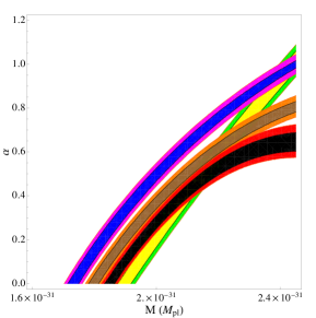
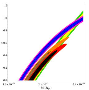
Figure 2: (Left panel) Analysis of the coupled exponential potential model of Eq. (4). The contours denote the 68.3 and 95.4 % C.L. allowed regions arising from a fit to SNIa data. The first three curves from left to right depict the results for $n=1,2$ and $n=4$. The last curve depicts the results arising from the fit to the uncoupled model. (Right panel) Same as in the left panel, but using the global fit results, i.e. the combined analysis to SNIa, CMB and BAO data sets.

Figure 2, left panel, shows the results of the $\chi^{2}$ analysis to SNIa data. In the right panel, the results for the global fit analysis are depicted. From left to right, the curves show the $68.3$ and $95.4\%$ C.L. allowed regions for the $n=1$, $n=2$, $n=4$ and the uncoupled ($\beta(\phi)=0$) cases. For this particular analysis the initial conditions for the scalar field are set to $\phi_{in}=M_{pl}$ and $\dot{\phi}_{in}=0$. We have checked the robustness of our results versus the scalar field initial conditions. Our conclusions remained unchanged, in agreement with the results of Ref. Bean et al. (2008b).

In general, larger values of $\alpha$ imply a smaller scalar potential. To compensate this effect, larger values of the amplitude of the potential $M$ are needed. This explains the shape of the degeneracy between $\alpha$ and $M$ in Fig. 2, being these two parameters positively correlated. For small values of both $M$ and $\alpha$, for instance, $(M,\alpha)\sim(1.8\,10^{-31}M_{pl},0.1)$, the ratio $V/\rho_{cr}^{0}$ appearing in the coupling term is smaller than one. When the value of $n$ is increased from 1 to 4, the uncoupled case behavior is recovered due the suppression of the coupling term $(V/\rho_{cr}^{0})^{n}$. Indeed, notice that the $n=4$ curve is almost superimposed to the uncoupled quintessence curve in Fig. 2 in the low $(M,\alpha)$ region.

For larger values of $\alpha$ and $M$ (within the allowed regions), the ratio $V/\rho_{cr}^{0}$ increases. The dark sector interaction becomes the dominant source term for the scalar field evolution in Eq. (2). In addition, the dark matter energy density, proportional to $\exp\left[\left(V(\phi)/\rho_{cr}^{0}\right)^{n}\right]$ (see Eq. (4)), starts to dominate the total energy density. Such a large contribution from the dark matter energy density is not compatible with SNIa data. This is precisely the reason for the bending of the curves in the left panel of Fig. 2. Notice that the shape of the curves for the coupled cases differs significantly from the uncoupled case for larger values of $\alpha$ and $M$ (within the allowed regions). The turn-over of the coupled model curves occurs at different values of the parameters $M$ and $\alpha$, depending on the value of the $n$ parameter. Namely, for $n=4$ the turn over shows up at smaller values of $M$ and $\alpha$ than those corresponding to the $n=1$ case. This is due to the fact that the $\beta(\phi)$ term given by Eq. (2) is proportional to $n$ and therefore the strength of the coupling term in this region of the $M$ and $\alpha$ parameters grows with $n$.

Notice, from the global fit results of Fig. 2 (right panel), that the allowed regions for large values of $n$, $\alpha$ and $M$ become significantly smaller than those arising from a fit exclusively to SNIa data. This is due to the CMB constraint which tends to favor smaller values of $M$ in both uncoupled and coupled cases. Indeed, larger values of $M$ are associated to very small values of the dark matter energy density, which directly influences the CMB shift parameter, see Eq. (12).

The best fit point for the uncoupled case is located at $(M,\alpha)=(2\,10^{-31}M_{pl},0.25)$ and it corresponds to $\Omega_{de}=0.72$ and $\Omega_{dm}=0.28$, being $\Omega_{de}$ and $\Omega_{dm}$ the current values of the dark matter and dark energy energy-densities, respectively. The equation of state of the dark energy field is $w_{\phi}=-1$. The associated global $\chi^{2}$ is $562$ compared to the $557$ effective degrees of freedom in our analysis. While for the $n=1$ coupled case the fit becomes weaker, it improves for larger values of $n$. For the $n=4$ coupled scenario, the best fit is associated to a $\chi^{2}=542$. However, the best fit point for the $n=4$ case corresponds to a cosmological constant scenario, since it is located at $\alpha=0$ and $M=1.85\,10^{-31}M_{pl}$, with the derived cosmological parameter values $\Omega_{de}=0.67,\Omega_{dm}=0.33$ and $w_{\phi}=-1$. Indeed, for $\Lambda$CDM universe we obtain $\chi^{2}=531$.

In summary, the cosmological data sets considered in the current analysis favor the large $n$ regime in a region of the $(M,\alpha)$ plane where both the coupling term and the dynamics of scalar field potential are negligible. In the next section we will explore the constraints from weak equivalence principle violation arguments.

V Weak equivalence principle constraints

Let us consider an interaction between fermionic dark matter, $\Psi$, and a light pseudo scalar boson, $\phi$, that interacts with the dark matter through a Yukawa coupling with strength $g$, described by the lagrangian

$$\mathcal{L} = i\bar{\Psi}\gamma_{\mu}\nabla^{\mu}\Psi-m_{\psi}\bar{\Psi}\Psi-\frac{1}{2}\nabla_{\mu}\phi\nabla^{\mu}\phi-V(\phi)+g\phi\bar{\Psi}\Psi~{},$$ (20)

where $m_{\psi}$ is the dark matter mass (independent of the scalar field). For $g\neq 0$, on scales smaller than $r_{s}=m_{\phi}^{-1}$, the Yukawa interaction acts like a long-range ‘fifth’ force in addition to gravity. The effective potential felt between two dark matter particles is

$$V(r)=-\frac{Gm_{\psi}^{2}}{r}\,\left[1+\alpha_{\rm Yuk}\exp\left(-\frac{r}{r_{s}}\right)\right]~{},$$ (21)

with

$$\alpha_{\rm Yuk} \equiv \frac{g^{2}}{4\pi}\frac{M_{pl}^{2}}{m_{\psi}^{2}}~{}.$$ (22)

The authors of Ref. Frieman and Gradwohl (1991) studied the impact of such a long-range interaction on both galaxy cluster masses and dark matter growth, reporting an upper bound of $\alpha_{\rm Yuk}\leq 1.3$ (for $\alpha_{\rm Yuk}>0$).

Kesden and Kamionkowski (K&K in the following) Kesden and Kamionkowski (2006a, b), analyzed the consequences of Weak Equivalence Principle (WEP) violation for dark-matter on galactic scales, focusing on dark-matter dominated satellite galaxies orbiting much larger host galaxies. They concluded that models in which the difference among dark matter and baryonic accelerations is larger than 10% are severely disfavoured. The relevant parameter constrained in K&K analysis is $\sqrt{\alpha_{\rm Yuk}}$. For reasonable models of the Sagittarius satellite galaxy tidal stream, K&K found an upper bound of $\alpha_{\rm Yuk}<0.04$, corresponding to

$$g/m_{\psi}<4.2\times 10^{-20}~{}{\rm GeV}^{-1}.$$ (23)

Since the K&K limit turns out to be the most stringent one, we exploit it here to set constraints on the exponential coupled model explored along the paper. We expand the interaction term $m_{dm}(\phi)\bar{\Psi}\Psi$, keeping only the linear terms in the scalar field. The former approximation is possible due to the fact that $\alpha\phi/M_{pl}\ll 1$ within the viable regions determined in the previous section. Therefore the linear term will clearly dominate the dark matter-scalar field interaction. We can write Eq. (4) as:

$$m_{dm}(\phi) = m_{0}\sum_{k=0}^{\infty}\frac{1}{k!}\left(\frac{V(\phi)}{\rho_{cr}^{0}}\right)^{kn},$$ (24)

$$V(\phi) \simeq M^{4}\left(1-\alpha\frac{\phi}{M_{pl}}\right)~{}.$$ (25)

It is straightforward to obtain an expression for both the fermion mass $m_{\psi}$ and the coupling $g$ in the Yukawa interaction term as defined in Eq. (20)

$$m_{\psi} = m_{0}\,\exp\left[\left(\frac{M^{4}}{\rho_{cr}}\right)^{n}\right]~{},$$ (26)

$$g = m_{\psi}\frac{n\alpha}{M_{pl}}\left(\frac{M^{4}}{\rho_{cr}}\right)^{n}~{}.$$ (27)

Therefore, if we express the amplitude of the potential as $M=\lambda\times 10^{-31}M_{pl}$, the limit of Eq. (23) becomes

$$\alpha<\frac{0.1\sqrt{8\pi}}{n\left(\frac{8\pi}{3}\frac{\lambda^{4}}{100}\right)^{n}}~{}.$$ (28)

For $\lambda=1.85$, which lies in the range of the viable regions obtained in Fig. 2, the former bound translates into a bound on the parameter $\alpha$ of the exponential coupled model of $\alpha<0.51,0.26$ and $0.14$ for $n=1,2$ and $4$, respectively. These bounds are stronger than those arising from cosmological observations and further restrict the allowed regions shown in Fig. 2. In addition, WEP bounds are complementary to cosmological constraints, since they have opposite trends: while cosmological bounds are rather loose when the amplitude of the potential increases, WEP limits get much stronger. Notice however that WEP bounds have been obtained using the strongest fifth force constraint, i.e. using the K&K limit. Mildest bounds on coupled quintessence models will arise if more conservative WEP bounds are applied.

VI Conclusions

We have studied a time varying-interaction among the dark matter and the dark energy sectors. The non-minimally coupled dark energy component is identified to a dynamical quintessence field, and it is coupled to the dark matter field via the dark matter mass term. The form of the interaction has been chosen to ensure an energy exchange between dark matter and dark energy proportional to the product of the dark matter energy density and the $n$th power of the scalar field potential. For a slowly rolling scalar field and $n=1$, the model presented here provides a possible effective lagrangian description of pure phenomenological quadratic interacting models such as the one studied in Ref. Boehmer et al. (2010).

The form for the scalar field self-interacting potential is assumed to be an exponential function of this field. The model has then been shown to possess a late time stable accelerated attractor regardless of the value of the $n$ parameter. We have also explored the constraints on this interacting model arising from the most recent SNIa, CMB and BAO data. While the fit improves slightly when allowing for a dark matter-dark energy interaction, the best fit point lies in a region in which both the coupling and the dynamics of the field are negligible. Therefore, current data does not favor this coupled dynamical model, even if it involves more parameters than the simplest cosmological scenario, i.e. a $\Lambda$CDM universe. A coupling between the two dark sectors can also be constrained by Weak Equivalence Principle violation arguments. We have derived the constraints arising from fifth-force searches. For the exponential potential coupled model studied in this paper, WEP constraints are very strong and much tighter than cosmological bounds.

References

- Damour et al. (1990) T. Damour, G. W. Gibbons, and C. Gundlach, Phys. Rev. Lett. 64, 123 (1990).
- Damour and Gundlach (1991) T. Damour and C. Gundlach, Phys. Rev. D43, 3873 (1991).
- Wetterich (1995) C. Wetterich, Astron. Astrophys. 301, 321 (1995), eprint hep-th/9408025.
- Amendola (2000) L. Amendola, Phys. Rev. D62, 043511 (2000), eprint astro-ph/9908023.
- Zimdahl and Pavon (2001) W. Zimdahl and D. Pavon, Phys. Lett. B521, 133 (2001), eprint astro-ph/0105479.
- Farrar and Peebles (2004) G. R. Farrar and P. J. E. Peebles, Astrophys. J. 604, 1 (2004), eprint astro-ph/0307316.
- Das et al. (2006) S. Das, P. S. Corasaniti, and J. Khoury, Phys. Rev. D73, 083509 (2006), eprint astro-ph/0510628.
- Zhang and Zhu (2006) H.-S. Zhang and Z.-H. Zhu, Phys. Rev. D73, 043518 (2006), eprint astro-ph/0509895.
- del Campo et al. (2006) S. del Campo, R. Herrera, G. Olivares, and D. Pavon, Phys. Rev. D74, 023501 (2006), eprint astro-ph/0606520.
- Bean et al. (2008a) R. Bean, E. E. Flanagan, and M. Trodden, New J. Phys. 10, 033006 (2008a), eprint 0709.1124.
- Olivares et al. (2008) G. Olivares, F. Atrio-Barandela, and D. Pavon, Phys. Rev. D77, 063513 (2008), eprint 0706.3860.
- Jackson et al. (2009) B. M. Jackson, A. Taylor, and A. Berera, Phys. Rev. D79, 043526 (2009), eprint 0901.3272.
- Koyama et al. (2009) K. Koyama, R. Maartens, and Y.-S. Song (2009), eprint 0907.2126.
- Boehmer et al. (2010) C. G. Boehmer, G. Caldera-Cabral, N. Chan, R. Lazkoz, and R. Maartens, Phys. Rev. D81, 083003 (2010), eprint 0911.3089.
- Carroll (1998) S. M. Carroll, Phys. Rev. Lett. 81, 3067 (1998), eprint astro-ph/9806099.
- Amendola (2004) L. Amendola, Phys. Rev. D69, 103524 (2004), eprint astro-ph/0311175.
- Amendola and Tocchini-Valentini (2001) L. Amendola and D. Tocchini-Valentini, Phys. Rev. D64, 043509 (2001), eprint astro-ph/0011243.
- Baldi (2010) M. Baldi (2010), eprint 1005.2188.
- Copeland et al. (1998) E. J. Copeland, A. R. Liddle, and D. Wands, Phys. Rev. D57, 4686 (1998), eprint gr-qc/9711068.
- Boehmer et al. (2008) C. G. Boehmer, G. Caldera-Cabral, R. Lazkoz, and R. Maartens, Phys. Rev. D78, 023505 (2008), eprint 0801.1565.
- Amanullah et al. (2010) R. Amanullah et al., Astrophys. J. 716, 712 (2010), eprint 1004.1711.
- Kowalski et al. (2008) M. Kowalski et al., Astrophys. J. 686, 749 (2008), eprint 0804.4142.
- Wang and Mukherjee (2006) Y. Wang and P. Mukherjee, Astrophys. J. 650, 1 (2006), eprint astro-ph/0604051.
- Eisenstein et al. (2005) D. J. Eisenstein et al. (SDSS), Astrophys. J. 633, 560 (2005), eprint astro-ph/0501171.
- Percival et al. (2007) W. J. Percival et al., Mon. Not. Roy. Astron. Soc. 381, 1053 (2007), eprint 0705.3323.
- Bean et al. (2008b) R. Bean, E. E. Flanagan, I. Laszlo, and M. Trodden, Phys. Rev. D78, 123514 (2008b), eprint 0808.1105.
- Frieman and Gradwohl (1991) J. A. Frieman and B.-A. Gradwohl, Phys. Rev. Lett. 67, 2926 (1991).