A Probabilistic Comparison of the Strength of Split, Triangle, and Quadrilateral Cuts (extended version)

Abstract

We consider mixed integer linear sets defined by two equations involving two integer variables and any number of non-negative continuous variables. The non-trivial valid inequalities of such sets can be classified into split, type 1, type 2, type 3, and quadrilateral inequalities. We use a strength measure of Goemans [11] to analyze the benefit from adding a non-split inequality on top of the split closure. Applying a probabilistic model, we show that the importance of a type 2 inequality decreases with decreasing lattice width, on average. Our results suggest that this is also true for type 3 and quadrilateral inequalities.

1 Introduction

We deal with the mixed integer set $P_{I}:=\{(x,s)\in{\mathbb{Z}}^{2}\times{\mathbb{R}}_{+}^{n}:x=f+\sum_{j=1}^{n}{r^{j}s_{j}}\}$ with $f\in{\mathbb{Q}}^{2}\setminus{\mathbb{Z}}^{2}$ and $r^{j}\in{\mathbb{Q}}^{2}\setminus\{0\}$ for all $j=1,\dots,n$. We refer to $f$ as the root vertex and to the vectors $r^{j}$ as rays. The motivation for analyzing $P_{I}$ is that it can be obtained as a relaxation of a general mixed integer linear set. Therefore, valid inequalities for ${\rm conv}(P_{I})$ give rise to cutting planes for the original mixed integer set. A thorough investigation of this model can be found in Andersen et al. [1, 2].

We consider the set $R_{f}(r^{1},\dots,r^{n}):={\rm conv}(\{s\in{\mathbb{R}}_{+}^{n}:f+\sum_{j=1}^{n}{r^{j}s_{j}}\in{\mathbb{Z}}^{2}\})$ which is the projection of ${\rm conv}(P_{I})$ onto the space of the $s$-variables. A closed convex set $B\subseteq{\mathbb{R}}^{2}$ with non-empty interior is lattice-free if the interior of $B$ is disjoint with ${\mathbb{Z}}^{2}$. Furthermore, $B$ is said to be maximal lattice-free if it is not properly contained in another lattice-free closed convex set. Any lattice-free polyhedron $B\subseteq{\mathbb{R}}^{2}$ with $f$ in its interior gives rise to a function $\psi^{B}:{\mathbb{R}}^{2}\mapsto{\mathbb{R}}_{+}$ which is the Minkowski functional of $B-f$. We recall that for a convex set $K$ containing the origin in its interior, the Minkowski functional $\|\cdot\|_{K}$ of $K$ is defined by $\|r\|_{K}:=\min\{\lambda>0:r\in\lambda K\}$ where $r\in{\mathbb{R}}^{2}$. We call $\sum_{j=1}^{n}{\psi^{B}(r^{j})s_{j}}\geq 1$ the cut associated with $B$. This inequality is valid for $R_{f}(r^{1},\dots,r^{n})$. Conversely, any non-trivial valid inequality for $R_{f}(r^{1},\dots,r^{n})$ can be obtained from a lattice-free polyhedron.

Every lattice-free rational polyhedron $B\subseteq{\mathbb{R}}^{2}$ with $f\in{\rm int}(B)$ is contained in a maximal lattice-free rational polyhedron $\bar{B}$. It follows that $\psi^{\bar{B}}(r^{j})\leq\psi^{B}(r^{j})$ for all $j=1,\dots,n$ and the cut associated with $B$ is dominated by the cut associated with $\bar{B}$. This implies that the benefit from adding the latter cut on top of the split closure is at least as high as the benefit from adding the former. In this paper, we focus exclusively on cuts associated with maximal lattice-free rational polyhedra.

A classification of planar maximal lattice-free closed convex sets was given by Lovász [14]. The refined classification which is stated below can be found in [10].

Proposition 1.1 ([10, 14])

Let $B$ be a maximal lattice-free closed convex set with non-empty interior. Then $B$ is a polyhedron and the relative interior of each facet of $B$ contains at least one integer point. In particular, $B$ is one of the following sets (see Fig. 1).

1. A split $\{(x_{1},x_{2})\in{\mathbb{R}}^{2}:b\leq a_{1}x_{1}+a_{2}x_{2}\leq b+1\}$ where $a_{1}$ and $a_{2}$ are coprime integers and $b$ is an integer.

2. A triangle which in turn is either

   1. a type 1 triangle, i.e. a triangle with integer vertices and exactly one integer point in the relative interior of each edge, or

   2. a type 2 triangle, i.e. a triangle with at least one fractional vertex $v$, exactly one integer point in the relative interior of the two edges incident to $v$ and at least two integer points on the third edge, or

   3. a type 3 triangle, i.e. a triangle with exactly three integer points on the boundary, one in the relative interior of each edge.

3. A quadrilateral containing exactly one integer point in the relative interior of each of its edges.

(a) Split

(b) Type 1 triangle

(c) Type 2 triangle

(d) Type 3 triangle

(e) Quadrilateral

Figure 1: All types of maximal lattice-free convex sets in ${\mathbb{R}}^{2}$ with non-empty interior.

By Proposition 1.1, it follows that $R_{f}(r^{1},\dots,r^{n})$ has three types of non-trivial valid inequalities: split, triangle, and quadrilateral inequalities named after the corresponding two-dimensional object from which the inequality can be derived as an intersection cut [5]. Triangle inequalities are further subdivided into type 1, type 2, and type 3 inequalities (see Fig. 1). Note that a non-trivial valid inequality for $R_{f}(r^{1},\dots,r^{n})$ can correspond to more than one maximal lattice-free polyhedron.

We are interested in the quality of cuts associated with the maximal lattice-free polyhedra described in Proposition 1.1. We use the strength measure introduced by Goemans [11] to evaluate the quality of a cut. Basu et al. [7] assess the strength of split, triangle, and quadrilateral inequalities in a non-probabilistic setting. They show that split and type 1 inequalities may produce an arbitrarily bad approximation of $R_{f}(r^{1},\dots,r^{n})$. On the other hand, type 2 or type 3 or quadrilateral inequalities deliver good approximations of $R_{f}(r^{1},\dots,r^{n})$ in terms of the strength. This, however comes with a price. Up to transformations preserving the integer lattice, there is only one split and only one triangle of type 1, but an infinite number of triangles of types 2 and 3 and quadrilaterals. Therefore, it can be expected that for real instances an approximation by adding all these cuts is hard to compute. From a more practical point of view, one is interested in approximations of the mixed integer hull that one can generate easily. Current state-of-the-art in computational integer programming is to experiment with split cuts and the split closure (see e.g. [3, 6]). This is the point of departure of our theoretical study.

The aim of this paper is to shed some light on the question which average improvement a non-split cut gives when added on top of the split closure. For that, we take any maximal lattice-free triangle or quadrilateral $B$, and we investigate all potential sets $R_{f}(r^{1},\dots,r^{n})$ such that we can generate a valid cut from $B$. For this, it is required that $f$ is in the interior of $B$. We vary $f$ uniformly at random in the interior of $B$. This is our probability distribution. For each particular $B$ and $f\in{\rm int}(B)$ we let $n$ and $r^{1},\dots,r^{n}$ attain arbitrary values. We compute a lower bound on the probability that the strength of adding the cut associated with $B$ on top of the split closure is less than or equal to an arbitrary value.

As a conclusion from our probabilistic analysis we obtain that the addition of a single type 2, type 3, or quadrilateral inequality to the split closure becomes less likely to be beneficial the closer the lattice-free set looks like a split, i.e. the closer its geometric width is to one.

We think that this complements nicely the analysis in [7]: they construct sequences of examples in which cuts from triangles of types 2 and 3, and quadrilaterals cannot be approximated to within a constant factor by the split closure. The approximation becomes worse as the triangles and quadrilaterals converge towards a split. From the results in our paper it follows that this geometrically counterintuitive situation occurs extremely rarely.

2 Probabilistic model and main results

Often, the quality of cuts is measured according to their worst case performance. In this paper we apply a stochastic approach by introducing a probability distribution on all possible instances. See [8] and [12] for other approaches on how to apply a probabilistic analysis to mixed integer linear sets.

Our aim is to evaluate the benefit from adding a single cut associated with a maximal lattice-free rational triangle or quadrilateral on top of the split closure. For that reason we apply the following strength measure.

A non-empty polyhedron $P=\left\{x\in{\mathbb{R}}_{+}^{n}:Ax\geq b\right\}$ is said to be of covering type if all entries in $A$ and $b$ are non-negative and $0\not\in P$. Let $\alpha\in(0,+\infty)$. We call $\alpha P:=\{x:\alpha x\in P\}$ the dilation of $P$ by the factor $\alpha$ and define $\alpha P:={\mathbb{R}}^{n}_{+}$ if $\alpha=+\infty$. Note that $P\subseteq\alpha P$ for $\alpha\geq 1$. Let $Q\subseteq{\mathbb{R}}^{n}_{+}$ be any convex set such that $P\subseteq Q$. The strength of $P$ with respect to $Q$, denoted by $t(P,Q)$, is the minimum value of $\alpha\geq 1$ such that $Q\subseteq\alpha P$.

Here, the underlying idea is that a high strength means high benefit. In other words, let $P$ and $Q$ be two relaxations for a mixed integer set $M$ such that $P\subseteq Q$. The larger $t(P,Q)$ the better is the gap to $M$ closed by $P$ compared to that of $Q$.

Lemma 2.1 ([11])

Let $P:=\{x\in{\mathbb{R}}_{+}^{n}:a_{i}^{T}x\geq b_{i}\ {\rm for\ all\ }i=1,\dots,m\}$ be a polyhedron of covering type and $Q\subseteq{\mathbb{R}}^{n}_{+}$ any convex set such that $P\subseteq Q$. Then,

$$t(P,Q)=\max_{i=1,\dots,m}\left\{\frac{b_{i}}{\inf\{a_{i}^{T}x:x\in Q\}}:b_{i}>0\right\}.$$

If $\inf\{a_{i}^{T}x:x\in Q\}=0$ for some $i\in\{1,\dots,m\}$, where $b_{i}>0$, then $t(P,Q)$ is defined to be $+\infty$.

In the following we use $R_{f}^{n}$ instead of $R_{f}(r^{1},\dots,r^{n})$ for simplicity. Note that $R_{f}^{n}$ is a polyhedron [15]. Let $\Omega$ be the set of all maximal lattice-free rational polyhedra in ${\mathbb{R}}^{2}$ which contain $f$ in the interior and let ${\cal S}$ (resp. ${\cal T}_{1}$, ${\cal T}_{2}$, ${\cal T}_{3}$, ${\cal Q}$) be the subset of $\Omega$ containing all splits (resp. triangles of type 1, type 2, type 3, quadrilaterals). Observe that $R_{f}^{n}=\{s\in{\mathbb{R}}^{n}_{+}:\sum_{j=1}^{n}{\psi^{B}(r^{j})s_{j}}\geq 1\textup{ for all }B\in{\cal S}\cup{\cal T}_{1}\cup{\cal T}_{2}\cup{\cal T}_{3}\cup{\cal Q}\}$. For a non-empty set ${\cal L}\subseteq\Omega$ we define ${\cal L}(R_{f}^{n})$ to be the intersection of all cuts associated with the polyhedra in ${\cal L}$ and the trivial inequalities $s_{j}\geq 0$ for all $j=1,\dots,n$. In the remainder of the paper, ${\cal L}$ will always be ${\cal S}$ or ${\cal S}\cup\{B\}$ for some $B\in\Omega\setminus{\cal S}$. In this case ${\cal L}(R_{f}^{n})$ is a polyhedron [9] of covering type.

In order to evaluate the gain from adding a triangle or quadrilateral inequality to the split closure we apply the following procedure. We fix a maximal lattice-free rational triangle or quadrilateral $B\in\Omega\setminus{\cal S}$, but we allow $f$ to vary in its interior. We will show that by considering a specific set of rays which depends only on $f$, we obtain an upper bound on $t({\cal F}(R_{f}^{n}),{\cal S}(R_{f}^{n}))$ where ${\cal F}={\cal S}\cup\{B\}$. Depending on where $f$ is located this bound may differ. By varying $f$ over the entire area of $B$ we compute the area for which the bound is below a certain value, $z$ say, and compare it to the area of $B$. This gives a ratio which is a lower bound on the probability that the strength is less than or equal to $z$. In turn, $1$ minus this probability is an upper bound for the chance that $B$ improves upon the split closure by a value of more than $z$ with respect to the strength.

Let $B\in\Omega\setminus{\cal S}$ and let ${\cal F}={\cal S}\cup\{B\}$. The following observation follows easily from Lemma 2.1.

Observation 2.1

$$t({\cal F}(R_{f}^{n}),{\cal S}(R_{f}^{n}))=\frac{1}{\min\{\sum_{j=1}^{n}{\psi^{B}(r^{j})s_{j}}:s\in{\cal S}(R_{f}^{n})\}}.$$

Since $B$, $f$, and $r^{1},\dots,r^{n}$ are rational, we can assume that the rays $r^{1},\dots,r^{n}$ are scaled such that the points $f+r^{j}$ are on the boundary of $B$ (see [7] for an explanation why this assumption is feasible). In the course of the paper we will deal with optimization problems of the following type:

$$\min\ \sum_{j=1}^{n}{\psi^{B}(r^{j})s_{j}\textup{\quad s.t.\quad}s\in{\cal S}(R_{f}^{n})}$$ (1)

for some $B\in\Omega\setminus{\cal S}$. Scaling the rays as described above implies that the objective function becomes $\sum_{j=1}^{n}{s_{j}}$.

We define a corner ray to be a ray $r^{j}$ where the point $f+r^{j}$ is a vertex of $B$. For now, assume that all the corner rays (and only those) are present. We will explain later why we can make this assumption. This implies that the corner rays are fixed once $f$ and $B$ are chosen. We assume a continuous uniform distribution on $f$ in the interior of $B$. Given $z\in{\mathbb{R}}$, $z>1$, we define $P^{B}(z)$ to be the probability that $t({\cal F}(R_{f}^{n}),{\cal S}(R_{f}^{n}))$ is less than or equal to $z$ for $f$ varying in the triangle or quadrilateral $B$, i.e.

$$P^{B}(z):=\frac{1}{{\rm Area}(B)}\int\limits_{f\in{\rm int}(B)}{\boldsymbol{1}\{t({\cal F}(R_{f}^{n}),{\cal S}(R_{f}^{n}))\leq z\}df},$$

where ${\rm Area}(B)$ is the area of $B$ and $\boldsymbol{1}$ is the indicator function.

Let us now argue why we can assume that all corner rays of $B$ are present in order to obtain the desired bound. Assume $k\geq 1$ corner rays $r^{n+1},\dots,r^{n+k}$ are missing and consider $R_{f}^{n+k}:={\rm conv}(\{s\in{\mathbb{R}}_{+}^{n+k}:f+\sum_{j=1}^{n+k}{r^{j}s_{j}}\in{\mathbb{Z}}^{2}\})$. We now apply Observation 2.1 to infer $t({\cal F}(R_{f}^{n+k}),{\cal S}(R_{f}^{n+k}))\geq t({\cal F}(R_{f}^{n}),{\cal S}(R_{f}^{n}))\Longleftrightarrow\min\{\sum_{j=1}^{n+k}{s_{j}}:s\in{\cal S}(R_{f}^{n+k})\}\leq\min\{\sum_{j=1}^{n}{s_{j}}:s\in{\cal S}(R_{f}^{n})\}$. The latter inequality follows from the fact that an optimal solution $\bar{s}$ for the latter minimization problem implies a feasible solution for the former minimization problem by setting $\bar{s}_{j}=0$ for all $j=n+1,\dots,n+k$. This is because if there would be a split which cuts off $(\bar{s},0)$ from ${\cal S}(R_{f}^{n+k})$, then the same split would cut off $\bar{s}$ from ${\cal S}(R_{f}^{n})$. It follows that $\boldsymbol{1}\{t({\cal F}(R_{f}^{n+k}),{\cal S}(R_{f}^{n+k}))\leq z\}\leq\boldsymbol{1}\{t({\cal F}(R_{f}^{n}),{\cal S}(R_{f}^{n}))\leq z\}$. Thus, by adding the corner rays we obtain a lower bound on $P^{B}(z)$.

We now explain why we can assume that only the corner rays of $B$ are present in order to compute $t({\cal F}(R_{f}^{n+k}),{\cal S}(R_{f}^{n+k}))$. In [7] it is shown that, if all corner rays are present and under the assumption of scaled rays, (1) reduces to the problem where only the corner rays are given, i.e. the objective function is $\sum_{j=1}^{k}{s_{j}}$, where $\{r^{1},\dots,r^{k}\}$, $k\in\{3,4\}$ is exactly the set of corner rays for the given triangle or quadrilateral $B$. By Observation 2.1 this implies $t({\cal F}(R_{f}^{n+k}),{\cal S}(R_{f}^{n+k}))=t({\cal F}(R_{f}^{k}),{\cal S}(R_{f}^{k}))$. Thus, in the remainder of the paper, in order to obtain the desired bounds, we assume that the set of rays consists of exactly the corner rays of $B$.

An important value in our analysis is the so-called lattice width. Let $B\subseteq{\mathbb{R}}^{2}$ be a maximal lattice-free set with non-empty interior. The lattice width of $B$ is defined to be

$$w(B):=\min_{u\in{\mathbb{Z}}^{2}\setminus\{0\}}\left\{\max_{x\in B}u^{T}x-\min_{x\in B}u^{T}x\right\}.$$ (2)

It is shown in [13] that $1\leq w(B)\leq 1+\frac{2}{\sqrt{3}}$. Furthermore, applying an affine unimodular transformation (i.e. a transformation preserving ${\mathbb{Z}}^{2}$) to $B$ changes neither the lattice width nor the strength. In the remainder of the paper, we informally call $B$ flat whenever $w(B)$ is sufficiently close to $1$. Our main results are summarized below.

Theorem 2.1 (probabilistic strength – lattice width relation)

Let $T_{i}$ be a triangle of type $i\in\{1,2\}$ and $w:=w(T_{2})$. Then, for any $z>1$, we have

1. $$P^{T_{1}}(z)=\begin{cases}0&\textup{if }1<z\leq\frac{3}{2},\\ \frac{3}{4}(\frac{2z-3}{z-1})^{2}&\textup{if }\frac{3}{2}<z<2,\\ 1&\textup{if }2\leq z<+\infty.\\ \end{cases}$$

2. $$P^{T_{2}}(z)\geq\begin{cases}0&\textup{if }1<z\leq w,\\[5.12149pt] g_{1}&\textup{if }w<z\leq\frac{w}{w-1},\\[5.12149pt] g_{1}+g_{2}&\textup{if }\frac{w}{w-1}<z<+\infty,\\ \end{cases}$$

   with $g_{1}=\frac{(z-w)(2wz-w-z)}{w^{2}(z-1)^{2}}$ and $g_{2}=\frac{(w-1)^{2}(z-1)^{2}-1}{w^{2}(z-1)^{2}}$.

Theorem 2.1 II shows that for any given $z>1$, $P^{T_{2}}(z)$ tends to $1$ if $w(T_{2})$ converges to $1$, i.e. the probability that a flat type 2 triangle improves upon the split closure by a value of more than $z$ goes to $0$. This will be explained in further detail in Section 5.

The analysis of a type 3 triangle $T_{3}$ and a quadrilateral $Q$ turns out to be more complex. We did not succeed in putting $P^{T_{3}}(z)$ (resp. $P^{Q}(z)$) into direct relation to $w(T_{3})$ (resp. $w(Q)$) and $z$ only. Instead we parametrize $T_{3}$ and $Q$ in terms of the coordinates of their vertices. Using this more complicated parametrization we derive formulas for $P^{T_{3}}(z)$ and $P^{Q}(z)$. Then we discretize the coordinates of the vertices and evaluate the formulas with respect to our discretization. This qualitatively leads to the same conclusion as before: if $T_{3}$ and $Q$ converge towards a split (meaning the lattice width converges to $1$), the probability that the strength of the associated inequality is less than or equal to $z$ tends to $1$. We refer to Sections 6 and 7 for the corresponding formulas.

3 Type 1 triangles

By an affine unimodular transformation, we assume that the type 1 triangle $T_{1}$ is given by $T_{1}={\rm conv}\{(0,0),(2,0),(0,2)\}$. Let $R_{1}:={\rm int}({\rm conv}\{(1,0),(0,1),(1,1)\})$, $R_{2}:={\rm int}({\rm conv}\{(0,0),(1,0),(0,1)\})$, $R_{3}:={\rm int}({\rm conv}\{(0,1),(1,1),(0,2)\})$, and $R_{4}:={\rm int}({\rm conv}\{(1,0),(1,1),(2,0)\})$.

Note that ${\rm int}(T_{1})\setminus\cup_{j=1}^{4}{R_{j}}$ is a set of area zero, so it can be neglected. For given $f\in R_{1}\cup R_{2}\cup R_{3}\cup R_{4}$ the three corner rays are $r^{1}=(-f_{1},-f_{2})$, $r^{2}=(2-f_{1},-f_{2})$, and $r^{3}=(-f_{1},2-f_{2})$. Let ${\cal F}={\cal S}\cup\{T_{1}\}$. In [7] it is shown that

$$t({\cal F}(R_{f}^{3}),{\cal S}(R_{f}^{3}))=\begin{cases}2&\textup{if }f\in R_{1},\\ \frac{3-f_{1}-f_{2}}{2-f_{1}-f_{2}}&\textup{if }f\in R_{2},\\ \frac{f_{2}+1}{f_{2}}&\textup{if }f\in R_{3},\\ \frac{f_{1}+1}{f_{1}}&\textup{if }f\in R_{4}.\\ \end{cases}$$ (3)

For the sake of a shorter notation we write $\boldsymbol{1}\{t\leq z\}$ instead of $\boldsymbol{1}\{t({\cal F}(R_{f}^{3}),{\cal S}(R_{f}^{3}))\leq z\}$. Then,

$$P^{T_{1}}(z)=\frac{1}{{\rm Area}(T_{1})}\sum_{j=1}^{4}{\int\limits_{f\in R_{j}}{\boldsymbol{1}\{t\leq z\}df}}.$$

We compute the four integrals separately. For that we need to check when the corresponding functions in (3) attain a value which is less than or equal to $z$. Assume $f\in R_{1}$. Then $\int_{f\in R_{1}}{\boldsymbol{1}\{t\leq z\}df}$ is $0$ if $z<2$ and is $\frac{1}{2}$ if $z\geq 2$. Assume $f\in R_{2}$. We have $\frac{3-f_{1}-f_{2}}{2-f_{1}-f_{2}}\leq z\Leftrightarrow f_{1}+f_{2}\leq\frac{2z-3}{z-1}$ and thus $\int_{f\in R_{2}}{\boldsymbol{1}\{t\leq z\}df}$ is $0$ if $z\leq\frac{3}{2}$, is $\frac{1}{2}$ if $z\geq 2$, and is $\frac{1}{2}(\frac{2z-3}{z-1})^{2}$ otherwise (here we used the fact that $0<f_{1}+f_{2}<1$ in $R_{2}$). Assume $f\in R_{3}$. Then $\frac{f_{2}+1}{f_{2}}\leq z\Leftrightarrow f_{2}\geq\frac{1}{z-1}$. Hence, $\int_{f\in R_{3}}{\boldsymbol{1}\{t\leq z\}df}$ is $0$ if $z\leq\frac{3}{2}$, is $\frac{1}{2}$ if $z\geq 2$, and is $\frac{1}{2}(\frac{2z-3}{z-1})^{2}$ otherwise (here we used $1<f_{2}<2$). Finally, the case $f\in R_{4}$ is analogous to the previous case. Since ${\rm Area}(T_{1})=2$ it follows

$$P^{T_{1}}(z)=\begin{cases}0&\textup{if }1<z\leq\frac{3}{2},\\ \frac{3}{4}(\frac{2z-3}{z-1})^{2}&\textup{if }\frac{3}{2}<z<2,\\ 1&\textup{if }2\leq z<+\infty.\\ \end{cases}$$

4 Proof strategy

The analysis of the strength of type 1 triangles is quite easy since the split closure is known: it is always defined by a subset of the three split inequalities corresponding to the splits whose normal vectors are the normal vectors of the facets of the type 1 triangle (see [7] for a proof). Note that $w(T_{1})=2$ and that this value is attained by precisely these vectors.

Using the split closure for triangles of types 2 and 3, and quadrilaterals would result in too complicated formulas. Thus, we choose another strategy. Instead of using the entire split closure we will take only one well-chosen split inequality and therefore obtain lower bounds for the desired probabilities. Let $B\in\Omega\setminus{\cal S}$. The split inequality which we choose will depend on the location of $f$ in the interior of $B$. For that we partition $B$ into regions $R_{1},\dots,R_{p}$ and select a single split for each region. The basic idea is to choose a split that contains $f$ in its interior and such that the normal vector of the split is a potential candidate for an integer vector for which $w(B)$ is attained. Our candidate splits will always be among the vectors $(1,0)$, $(0,1)$, and $(1,1)$ since we apply an affine unimodular transformation to $B$ to bring it into an appropriate form (see Sections 5, 6, and 7 for details).

We now show that our simplification of using only one split inequality instead of the split closure leads to a lower bound for $P^{B}(z)$. Let ${\cal F}={\cal S}\cup\{B\}$ for some $B\in\Omega\setminus{\cal S}$ and let $L\in{\cal S}$ be arbitrary. Then, by Observation 2.1, $t({\cal F}(R_{f}^{k}),{\cal S}(R_{f}^{k}))=(\min\{\sum_{j=1}^{k}{s_{j}}:s\in{\cal S}(R_{f}^{k})\})^{-1}\leq(\min\{\sum_{j=1}^{k}{s_{j}}:s_{j}\geq 0\textup{ for }j\in\{1,\dots,k\}\textup{ and }\sum_{j=1}^{k}{\psi^{L}(r^{j})s_{j}}\geq 1\})^{-1}=t(\{\sum_{j=1}^{k}{\psi^{L}(r^{j})s_{j}}\geq 1,\sum_{j=1}^{k}{\psi^{B}(r^{j})s_{j}}\geq 1\}\cap\{s_{j}\geq 0\textup{ for }j\in\{1,\dots,k\}\},\{\sum_{j=1}^{k}{\psi^{L}(r^{j})s_{j}}\geq 1\}\cap\{s_{j}\geq 0\textup{ for }j\in\{1,\dots,k\}\})$, since we assumed $\psi^{B}(r^{j})=1$ for all $j=1,\dots,k$.

For ease of notation we denote the latter by $\bar{t}(B,L)$, which is the strength of the polyhedron obtained by adding the cuts associated with $B$ and $L$ with respect to the polyhedron obtained by just adding the cut associated with $L$. It follows $\boldsymbol{1}\{t({\cal F}(R_{f}^{k}),{\cal S}(R_{f}^{k}))\leq z\}\geq\boldsymbol{1}\{\bar{t}(B,L)\leq z\}$ and therefore

$$P^{B}(z)\geq\frac{1}{{\rm Area}(B)}\sum_{j=1}^{p}{\int\limits_{f\in R_{j}}{\boldsymbol{1}\{\bar{t}(B,L_{R_{j}})\leq z\}df}},$$ (4)

where $L_{R_{j}}$ is the single split which is used in region $R_{j}$ to approximate the split closure, for $j=1,\dots,p$. In the following, for simplicity, we write $\boldsymbol{1}\{\bar{t}\leq z\}$ instead of $\boldsymbol{1}\{\bar{t}(B,L)\leq z\}$ whenever $B$ and $L$ are clear from the context. In order to compute $\bar{t}(B,L)$ we need to solve an optimization problem of the type

$$\begin{split}\min\ &s_{1}+\dots+s_{k}\\ \mbox{\quad s.t. }&\psi^{L}(r^{1})s_{1}+\dots+\psi^{L}(r^{k})s_{k}\geq 1,\\ &s_{j}\geq 0\quad\mbox{for }j=1,\dots,k.\end{split}$$

The values $\psi^{L}(r^{1}),\dots,\psi^{L}(r^{k})$ are called the coefficients of the split $L$. In general, for a split $L=\{x\in{\mathbb{R}}^{2}:\left\lfloor\pi^{T}f\right\rfloor\leq\pi^{T}x\leq\left\lceil\pi^{T}f\right\rceil\}$, $\pi\in{\mathbb{Z}}^{2}\setminus\{0\}$, containing $f$ in its interior and with corresponding inequality $\sum_{j=1}^{k}\psi^{L}(r^{j})s_{j}\geq 1$, it is easy to verify that

$$\psi^{L}(r^{j})=\begin{cases}\tfrac{\pi^{T}r^{j}}{\left\lceil\pi^{T}f\right\rceil-\pi^{T}f}&\textup{if }\pi^{T}r^{j}>0,\\ 0&\textup{if }\pi^{T}r^{j}=0,\\ \tfrac{\pi^{T}r^{j}}{\left\lfloor\pi^{T}f\right\rfloor-\pi^{T}f}&\textup{if }\pi^{T}r^{j}<0.\end{cases}$$ (5)

Thus, we just need the normal vector $\pi$ of the split $L$ to compute the split coefficients $\psi^{L}(r^{1}),\dots,\psi^{L}(r^{k})$.

In Section 5 we will explain our computations for triangles of type 2 in detail. Since the computations for quadrilaterals and triangles of type 3 in Sections 6 and 7 give no new insights we will only state intermediate results there.

5 Type 2 triangles

By an affine unimodular transformation, we assume that the type 2 triangle $T_{2}$ has one facet containing the points $(0,0)$ and $(1,0)$, one facet containing $(0,1)$, and one facet containing $(1,1)$. Furthermore, one vertex $a=(a_{1},a_{2})$ satisfies $0<a_{1}<1$ and $1<a_{2}$. Thus, the other vertices are $(-\frac{a_{1}}{a_{2}-1},0)$ and $(\frac{a_{2}-a_{1}}{a_{2}-1},0)$. We assume that $a$ is arbitrary but fixed and treat it as a parameter in the subsequent computations. We decompose $T_{2}$ into six regions: $R_{1}:={\rm int}({\rm conv}\{(0,0),(a_{1},0),(a_{1},1),(0,1)\})$, $R_{2}:={\rm int}({\rm conv}\{(a_{1},0),(1,0),(1,1),(a_{1},1)\})$, $R_{3}:={\rm int}({\rm conv}\{(0,0),(0,1),(-\frac{a_{1}}{a_{2}-1},0)\})$, $R_{4}:={\rm int}({\rm conv}\{(1,0),$ $(1,1),(\frac{a_{2}-a_{1}}{a_{2}-1},0)\})$, $R_{5}:={\rm int}({\rm conv}\{(0,1),(a_{1},1),(a_{1},a_{2})\})$, and $R_{6}:={\rm int}({\rm conv}\{(a_{1},1),(1,1),(a_{1},a_{2})\})$ (see Fig. 2).

Figure 2: Decomposition of a type 2 triangle.

For given $f\in\cup_{j=1}^{6}{R_{j}}$ the three corner rays are $r^{1}=(-\frac{a_{1}}{a_{2}-1}-f_{1},-f_{2})$, $r^{2}=(\frac{a_{2}-a_{1}}{a_{2}-1}-f_{1},-f_{2})$, and $r^{3}=(a_{1}-f_{1},a_{2}-f_{2})$. Furthermore, ${\rm Area}(T_{2})=\frac{(a_{2})^{2}}{2(a_{2}-1)}$. Our assumptions on $T_{2}$ imply that $w(T_{2})$, as defined in (2), is attained for $u=(1,0)$ or $u=(0,1)$ (see [4]). Thus, $w:=w(T_{2})=\min\{a_{2},\frac{a_{2}}{a_{2}-1}\}$ which implies $w=a_{2}$ if $a_{2}\leq 2$ and $w=\frac{a_{2}}{a_{2}-1}$ if $a_{2}>2$. In either case we have ${\rm Area}(T_{2})=\frac{w^{2}}{2(w-1)}$.

In regions $R_{3}$ and $R_{4}$ we use the split $S_{1}:=\{(x_{1},x_{2})\in{\mathbb{R}}^{2}:0\leq x_{2}\leq 1\}$ and in regions $R_{5}$ and $R_{6}$ we use the split $S_{2}:=\{(x_{1},x_{2})\in{\mathbb{R}}^{2}:0\leq x_{1}\leq 1\}$. In regions $R_{1}$ and $R_{2}$ we choose either $S_{1}$ or $S_{2}$. We will use the one whose normal vector attains $w$, i.e. we choose $S_{1}$ if $a_{2}\leq 2$ and $S_{2}$ if $a_{2}>2$. Note that our choice of the single split which is taken instead of the split closure is such that it attains minimal lattice width with respect to $T_{2}$. Such a split has another nice property: among all splits that contain $f$ in their interior we select one which covers most of the area of the triangle.

5.1 Regions $R_{3}$ and $R_{4}$

Let $f\in R_{3}\cup R_{4}$. In order to compute $\bar{t}(T_{2},S_{1})$ we have to solve the optimization problem

$$\begin{split}\min\ &s_{1}+s_{2}+s_{3}\\ \mbox{\quad s.t. }&\psi^{S_{1}}(r^{1})s_{1}+\psi^{S_{1}}(r^{2})s_{2}+\psi^{S_{1}}(r^{3})s_{3}\geq 1,\\ &s_{j}\geq 0\quad\mbox{for }j=1,2,3.\end{split}$$ (6)

Since we use $S_{1}$ we have $\pi=(0,1)$ and since $f\in R_{3}\cup R_{4}$ it holds $0<\pi^{T}f<1$. Thus, using (5), we obtain $\psi^{S_{1}}(r^{1})=\psi^{S_{1}}(r^{2})=1$ and $\psi^{S_{1}}(r^{3})=\frac{a_{2}-f_{2}}{1-f_{2}}$. Therefore, an optimal solution to (6) is $s^{\ast}=(0,0,\frac{1-f_{2}}{a_{2}-f_{2}})$ with optimal objective value $\frac{1-f_{2}}{a_{2}-f_{2}}$. It follows $\bar{t}(T_{2},S_{1})=\frac{a_{2}-f_{2}}{1-f_{2}}$ for $f\in R_{3}\cup R_{4}$.

5.2 Regions $R_{5}$ and $R_{6}$

Let $f\in R_{5}$. To compute $\bar{t}(T_{2},S_{2})$ in this case we solve the optimization problem $\min\ \sum_{j=1}^{3}{s_{j}}$ such that $\sum_{j=1}^{3}{\psi^{S_{2}}(r^{j})s_{j}}\geq 1,\ s_{j}\geq 0$ for $j=1,2,3$. Applying (5) we obtain $\psi^{S_{2}}(r^{1})=\frac{f_{1}+\frac{a_{1}}{a_{2}-1}}{f_{1}}$, $\psi^{S_{2}}(r^{2})=\frac{\frac{a_{2}-a_{1}}{a_{2}-1}-f_{1}}{1-f_{1}}$, and $\psi^{S_{2}}(r^{3})=\frac{a_{1}-f_{1}}{1-f_{1}}$. Hence, the optimal solution is the minimum among $\{(\psi^{S_{2}}(r^{1}))^{-1}$, $(\psi^{S_{2}}(r^{2}))^{-1}$, $(\psi^{S_{2}}(r^{3}))^{-1}\}$. Using our assumptions on the variables and parameters it follows $(\psi^{S_{2}}(r^{3}))^{-1}$ $\geq 1$ and $(\psi^{S_{2}}(r^{i}))^{-1}\leq 1$ for $i\in\{1,2\}$. One easily verifies that $(\psi^{S_{2}}(r^{1}))^{-1}\leq(\psi^{S_{2}}(r^{2}))^{-1}\Leftrightarrow a_{1}\geq f_{1}$ which is satisfied in $R_{5}$ by assumption. Thus, $\bar{t}(T_{2},S_{2})=\frac{f_{1}+\frac{a_{1}}{a_{2}-1}}{f_{1}}$ for $f\in R_{5}$.

Let $f\in R_{6}$. By symmetry, i.e. $a_{1}\rightarrow 1-a_{1}$ and $f_{1}\rightarrow 1-f_{1}$, we obtain $\bar{t}(T_{2},S_{2})=\frac{\frac{a_{2}-a_{1}}{a_{2}-1}-f_{1}}{1-f_{1}}$ for $f\in R_{6}$.

5.3 Regions $R_{1}$ and $R_{2}$

First assume $a_{2}\leq 2$ and use the split $S_{1}$. Let $f\in R_{1}\cup R_{2}$. The associated optimization problem is $\min\ \sum_{j=1}^{3}{s_{j}}$ s.t. $\sum_{j=1}^{3}{\psi^{S_{1}}(r^{j})s_{j}}\geq 1,\ s_{j}\geq 0$ for $j=1,2,3$ with $\psi^{S_{1}}(r^{1})=\psi^{S_{1}}(r^{2})=1$ and $\psi^{S_{1}}(r^{3})=\frac{a_{2}-f_{2}}{1-f_{2}}$. Hence, $\bar{t}(T_{2},S_{1})=\frac{a_{2}-f_{2}}{1-f_{2}}$ for $f\in R_{1}\cup R_{2}$ and $a_{2}\leq 2$.

Now assume that $a_{2}>2$. We use the split $S_{2}$. Let $f\in R_{1}$. The solution of the optimization problem $\min\ \sum_{j=1}^{3}{s_{j}}$ s.t. $\sum_{j=1}^{3}{\psi^{S_{2}}(r^{j})s_{j}}\geq 1,\ s_{j}\geq 0$ for $j=1,2,3$ with $\psi^{S_{2}}(r^{1})=\frac{f_{1}+\frac{a_{1}}{a_{2}-1}}{f_{1}}$, $\psi^{S_{2}}(r^{2})=\frac{\frac{a_{2}-a_{1}}{a_{2}-1}-f_{1}}{1-f_{1}}$, and $\psi^{S_{2}}(r^{3})=\frac{a_{1}-f_{1}}{1-f_{1}}$ is the minimum of the set $\{(\psi^{S_{2}}(r^{1}))^{-1},(\psi^{S_{2}}(r^{2}))^{-1}\}$ as $(\psi^{S_{2}}(r^{3}))^{-1}\geq 1$. It is easy to verify that $(\psi^{S_{2}}(r^{1}))^{-1}\leq(\psi^{S_{2}}(r^{2}))^{-1}\Leftrightarrow a_{1}\geq f_{1}$. Therefore, we have $\bar{t}(T_{2},S_{2})=\frac{f_{1}+\frac{a_{1}}{a_{2}-1}}{f_{1}}$ for $f\in R_{1}$ and $a_{2}>2$.

Finally, assume $f\in R_{2}$. By symmetry, we obtain $\bar{t}(T_{2},S_{2})=\frac{\frac{a_{2}-a_{1}}{a_{2}-1}-f_{1}}{1-f_{1}}$ for $f\in R_{2}$ and $a_{2}>2$.

The following table summarizes the function $\bar{t}(T_{2},S_{i})$, for the corresponding $i\in\{1,2\}$.

$\begin{array}[]{c|c|l}\textup{$\bar{t}(T_{2},S_{i})$}&\textup{$\bar{t}(T_{2},S_{i})$}&\textup{Location of $f$}\\ \textup{for $a_{2}\leq 2$}&\textup{for $a_{2}>2$}&\\ \hline\cr&&\\[-8.53581pt] \frac{a_{2}-f_{2}}{1-f_{2}}&\frac{f_{1}+\frac{a_{1}}{a_{2}-1}}{f_{1}}&f\in R_{1}\\ \frac{a_{2}-f_{2}}{1-f_{2}}&\frac{\frac{a_{2}-a_{1}}{a_{2}-1}-f_{1}}{1-f_{1}}&f\in R_{2}\\ \frac{a_{2}-f_{2}}{1-f_{2}}&\frac{a_{2}-f_{2}}{1-f_{2}}&f\in R_{3}\\ \frac{a_{2}-f_{2}}{1-f_{2}}&\frac{a_{2}-f_{2}}{1-f_{2}}&f\in R_{4}\\ \frac{f_{1}+\frac{a_{1}}{a_{2}-1}}{f_{1}}&\frac{f_{1}+\frac{a_{1}}{a_{2}-1}}{f_{1}}&f\in R_{5}\\ \frac{\frac{a_{2}-a_{1}}{a_{2}-1}-f_{1}}{1-f_{1}}&\frac{\frac{a_{2}-a_{1}}{a_{2}-1}-f_{1}}{1-f_{1}}&f\in R_{6}\end{array}$

5.4 Approximation for $P^{T_{2}}(z)$

We compute the integrals $\int_{f\in R_{j}}{\boldsymbol{1}\{\bar{t}(T_{2},S_{i})\leq z\}df}$ for $j\in\{1,\dots,6\}$ and the corresponding split $S_{1}$ or $S_{2}$ which we used above. For simplicity, $\int_{f\in R_{j}}:=\int_{f\in R_{j}}{\boldsymbol{1}\{\bar{t}\leq z\}df}$ for $j=1,\dots,6$.

Let $f\in R_{3}$. Then $\boldsymbol{1}\{\bar{t}\leq z\}=1\Leftrightarrow\frac{a_{2}-f_{2}}{1-f_{2}}\leq z\Leftrightarrow f_{2}\leq\frac{z-a_{2}}{z-1}$. Observe that $\int_{f\in R_{3}}=0$ if $z\leq a_{2}$. If $z>a_{2}$, then the area of the set $\{f\in R_{3}:f_{2}\leq\frac{z-a_{2}}{z-1}\}$ is the difference of the area of two triangles (see Fig. 3(d)). Direct computations yield

$$\int\limits_{f\in R_{3}}=\begin{cases}0&\textup{if }z\leq a_{2},\\ \frac{a_{1}(z-a_{2})(z+a_{2}-2)}{2(a_{2}-1)(z-1)^{2}}&\textup{if }z>a_{2}.\\ \end{cases}$$

Let $f\in R_{5}$. Then $\boldsymbol{1}\{\bar{t}\leq z\}=1\Leftrightarrow\frac{f_{1}+\frac{a_{1}}{a_{2}-1}}{f_{1}}\leq z\Leftrightarrow f_{1}\geq\frac{a_{1}}{(a_{2}-1)(z-1)}$. We have $\int_{f\in R_{5}}=0\Leftrightarrow\frac{a_{1}}{(a_{2}-1)(z-1)}\geq a_{1}\Leftrightarrow z\leq\frac{a_{2}}{a_{2}-1}$. If $z>\frac{a_{2}}{a_{2}-1}$, then again we compute the difference of the area of two triangles (see Fig. 3(f)) and infer

$$\int\limits_{f\in R_{5}}=\begin{cases}0&\textup{if }z\leq\frac{a_{2}}{a_{2}-1},\\ \frac{a_{1}(a_{2}-1)}{2}g_{3}&\textup{if }z>\frac{a_{2}}{a_{2}-1},\\ \end{cases}$$

where $g_{3}=1-\frac{1}{(a_{2}-1)^{2}(z-1)^{2}}$.

By symmetry, the integrals for $f\in R_{4}$ and $f\in R_{6}$ are obtained by replacing $a_{1}$ with $1-a_{1}$ in the formulas for $R_{3}$ and $R_{5}$ (see Fig. 3(e) and 3(g)). Thus,

$$\int\limits_{f\in R_{4}} =\begin{cases}0&\textup{if }z\leq a_{2},\\ \frac{(1-a_{1})(z-a_{2})(z+a_{2}-2)}{2(a_{2}-1)(z-1)^{2}}&\textup{if }z>a_{2},\\ \end{cases}$$

$$\int\limits_{f\in R_{6}} =\begin{cases}0&\textup{if }z\leq\frac{a_{2}}{a_{2}-1},\\ \frac{(1-a_{1})(a_{2}-1)}{2}g_{3}&\textup{if }z>\frac{a_{2}}{a_{2}-1}.\\ \end{cases}$$

In order to compute $\int_{f\in R_{i}}$ for $i=1,2$ we distinguish the cases $a_{2}\leq 2$ and $a_{2}>2$. First, let us assume that $a_{2}\leq 2$. Computations in a similar manner as above (area of the shaded quadrilateral in Fig. 3(a)) lead to

$$\int\limits_{f\in R_{1}} =\begin{cases}0&\textup{if }z\leq a_{2},\\ \frac{a_{1}(z-a_{2})}{z-1}&\textup{if }z>a_{2},\\ \end{cases}$$

$$\int\limits_{f\in R_{2}} =\begin{cases}0&\textup{if }z\leq a_{2},\\ \frac{(1-a_{1})(z-a_{2})}{z-1}&\textup{if }z>a_{2}.\\ \end{cases}$$

Now let us assume that $a_{2}>2$. Computing the corresponding area (see Fig. 3(b) and 3(c)) yields

$$\int\limits_{f\in R_{1}} =\begin{cases}0&\textup{if }z\leq\frac{a_{2}}{a_{2}-1},\\ a_{1}g_{4}&\textup{if }z>\frac{a_{2}}{a_{2}-1},\\ \end{cases}$$

$$\int\limits_{f\in R_{2}} =\begin{cases}0&\textup{if }z\leq\frac{a_{2}}{a_{2}-1},\\ (1-a_{1})g_{4}&\textup{if }z>\frac{a_{2}}{a_{2}-1},\\ \end{cases}$$

where $g_{4}=1-\frac{1}{(a_{2}-1)(z-1)}$.

(a) $R_{1}$ and $R_{2}$ for $a_{2}\leq 2$

(b) $R_{1}$ for $a_{2}>2$

(c) $R_{2}$ for $a_{2}>2$

(d) $R_{3}$

(e) $R_{4}$

(f) $R_{5}$

(g) $R_{6}$

Figure 3: The shaded regions satisfy $\boldsymbol{1}\{\bar{t}\leq z\}=1$.

We can aggregate the formulas for regions $R_{1}$ and $R_{2}$, $R_{3}$ and $R_{4}$, and $R_{5}$ and $R_{6}$ in order to eliminate the parameter $a_{1}$. It follows

$$\int\limits_{f\in R_{1}}+\int\limits_{f\in R_{2}} =\begin{cases}0&\textup{if }z\leq a_{2}\textup{ and }a_{2}\leq 2,\\ \frac{z-a_{2}}{z-1}&\textup{if }z>a_{2}\textup{ and }a_{2}\leq 2,\\ \end{cases}$$

$$\int\limits_{f\in R_{1}}+\int\limits_{f\in R_{2}} =\begin{cases}0&\textup{if }z\leq\frac{a_{2}}{a_{2}-1}\textup{ and }a_{2}>2,\\ 1-\frac{1}{(a_{2}-1)(z-1)}&\textup{if }z>\frac{a_{2}}{a_{2}-1}\textup{ and }a_{2}>2,\\ \end{cases}$$

$$\int\limits_{f\in R_{3}}+\int\limits_{f\in R_{4}} =\begin{cases}0&\textup{if }z\leq a_{2},\\ \frac{(z-a_{2})(z+a_{2}-2)}{2(a_{2}-1)(z-1)^{2}}&\textup{if }z>a_{2},\\ \end{cases}$$

$$\int\limits_{f\in R_{5}}+\int\limits_{f\in R_{6}} =\begin{cases}0&\textup{if }z\leq\frac{a_{2}}{a_{2}-1},\\ \frac{a_{2}-1}{2}\left(1-\frac{1}{(a_{2}-1)^{2}(z-1)^{2}}\right)&\textup{if }z>\frac{a_{2}}{a_{2}-1}.\\ \end{cases}$$

We are now ready to state our results in terms of the lattice width. Reinterpreting the formulas above we obtain for $a_{2}\leq 2$ (i.e. $w=a_{2}$) the integrals

$$\int\limits_{f\in R_{1}}+\int\limits_{f\in R_{2}} =\begin{cases}0&\textup{if }z\leq w,\\ \frac{z-w}{z-1}&\textup{if }z>w,\\ \end{cases}$$

$$\int\limits_{f\in R_{3}}+\int\limits_{f\in R_{4}} =\begin{cases}0&\textup{if }z\leq w,\\ \frac{(z-w)(z+w-2)}{2(w-1)(z-1)^{2}}&\textup{if }z>w,\\ \end{cases}$$

$$\int\limits_{f\in R_{5}}+\int\limits_{f\in R_{6}} =\begin{cases}0&\textup{if }z\leq\frac{w}{w-1},\\ \frac{(w-1)^{2}(z-1)^{2}-1}{2(w-1)(z-1)^{2}}&\textup{if }z>\frac{w}{w-1}.\\ \end{cases}$$

For $a_{2}>2$ (i.e. $w=\frac{a_{2}}{a_{2}-1}$) we have

$$\int\limits_{f\in R_{1}}+\int\limits_{f\in R_{2}} =\begin{cases}0&\textup{if }z\leq w,\\ \frac{z-w}{z-1}&\textup{if }z>w,\\ \end{cases}$$

$$\int\limits_{f\in R_{3}}+\int\limits_{f\in R_{4}} =\begin{cases}0&\textup{if }z\leq\frac{w}{w-1},\\ \frac{(w-1)^{2}(z-1)^{2}-1}{2(w-1)(z-1)^{2}}&\textup{if }z>\frac{w}{w-1},\\ \end{cases}$$

$$\int\limits_{f\in R_{5}}+\int\limits_{f\in R_{6}} =\begin{cases}0&\textup{if }z\leq w,\\ \frac{(z-w)(z+w-2)}{2(w-1)(z-1)^{2}}&\textup{if }z>w.\\ \end{cases}$$

Note that $w\leq\frac{w}{w-1}$ as $w\leq 2$ (see [4] for a proof that any triangle of type 2 satisfies $1<w\leq 2$). Hence, together with (4) we arrive at the following formula.

$$P^{T_{2}}(z)\geq\begin{cases}0&\textup{if }1<z\leq w,\\[5.12149pt] g_{1}&\textup{if }w<z\leq\frac{w}{w-1},\\[5.12149pt] g_{1}+g_{2}&\textup{if }\frac{w}{w-1}<z<+\infty,\\ \end{cases}$$ (7)

with $g_{1}=\frac{(z-w)(2wz-w-z)}{w^{2}(z-1)^{2}}$ and $g_{2}=\frac{(w-1)^{2}(z-1)^{2}-1}{w^{2}(z-1)^{2}}$. Let $z>1$ be given. We want to show that the probability to improve upon the split closure by a value of more than $z$ when adding a type 2 triangle becomes the smaller the closer the type 2 triangle is to a split, i.e. the closer $w$ is to $1$. For $w$ being sufficiently close to $1$ we have $w<z\leq\frac{w}{w-1}$. Just substitute $1$ for $w$ in (7) to infer that $P^{T_{2}}(z)$ converges to $1$ for any $z>1$. Therefore, $1-P^{T_{2}}(z)$ tends to $0$. In other words, the chance that adding a flat type 2 triangle improves the split closure by a value of more than $z$ with respect to our strength measure tends to $0$. In terms of the vertex $(a_{1},a_{2})$ this happens if $a_{2}$ converges either to $1$ (i.e. $T_{2}$ converges to $S_{1}$) or infinity (i.e. $T_{2}$ converges to $S_{2}$).

Two special cases are of interest: $z=2$ and $z=\frac{3}{2}$. Plugging in $z=2$ in (7) yields $1-P^{T_{2}}(2)\leq\frac{4(w-1)^{2}}{w^{2}}$ for any $1<w\leq 2$ (see Fig. 4(a)) and plugging in $z=\frac{3}{2}$ in (7) leads to

$$P^{T_{2}}\left(\frac{3}{2}\right)\geq\begin{cases}0&\textup{if }\frac{3}{2}\leq w\leq 2,\\ \frac{(3-2w)(4w-3)}{w^{2}}&\textup{if }1<w<\frac{3}{2}\\ \end{cases}$$

(see Fig. 4(b)). $1-P^{T_{2}}(2)$ is interpretable as the probability that the inequality corresponding to $T_{2}$ closes more gap to $R_{f}^{3}$ than the inequality corresponding to any type 1 triangle. On the other hand $P^{T_{2}}(\frac{3}{2})$ can be seen as the probability that adding $T_{2}$ to the split closure is inferior to adding any type 1 triangle $T_{1}$ with rays going through the corners of $T_{1}$.

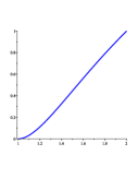
(a) An upper bound for $1-P^{T_{2}}(2)$ in terms of $w$.

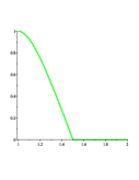
(b) A lower bound for $P^{T_{2}}(\frac{3}{2})$ in terms of $w$.

Figure 4: Bounds for $1-P^{T_{2}}(2)$ and $P^{T_{2}}(\frac{3}{2})$.

The interpretation is based on the fact that any type 1 triangle (assuming corner rays) has a strength between $\frac{3}{2}$ and $2$. On the one hand type 1 triangles are inferior to flat type 2 triangles by comparing the worst case strength (see [7]). On the other hand a type 1 triangle guarantees a strength of $\frac{3}{2}$ and is therefore superior to a flat type 2 triangle on average. For instance, let $T_{2}$ be a type 2 triangle with $w(T_{2})=1{.}1$. Then $1-P^{T_{2}}(2)<3{.}4\%$ and $P^{T_{2}}(\frac{3}{2})>92{.}5\%$. Thus, with a probability of less than $3{.}4\%$, $T_{2}$ is better than any type 1 triangle $T_{1}$, and worse with a probability of more than $92{.}5\%$ if corner rays are assumed for $T_{1}$. We point out that these probabilities are quite close to $0$ and $1$, respectively, even though we used just one split instead of the entire split closure.

6 Quadrilaterals

The vertices of the quadrilateral $Q$ are denoted $a=(a_{1},a_{2})$, $b=(b_{1},b_{2})$, $c=(c_{1},c_{2})$, and $d=(d_{1},d_{2})$. By an affine unimodular transformation, we assume that the point $(0,0)$ (resp. $(1,0)$, $(0,1)$, $(1,1)$) is in the relative interior of the facet with vertices $b$ and $c$ (resp. $b$ and $d$, $a$ and $c$, $a$ and $d$). We further assume $0<a_{1}\leq b_{1}<1$, $1<a_{2}$, $b_{2}<0$, and $-b_{2}\leq a_{2}-1$. The parameters $a_{1}$, $a_{2}$, $b_{1}$, and $b_{2}$ are assumed to be arbitrary but fixed. This implies $c_{1}=-\frac{a_{1}b_{1}}{(a_{2}-1)b_{1}-a_{1}b_{2}}$, $c_{2}=\frac{c_{1}b_{2}}{b_{1}}$, $d_{1}=\frac{(a_{2}-a_{1})(1-b_{1})-(1-a_{1})b_{2}}{(a_{2}-1)(1-b_{1})-(1-a_{1})b_{2}}$, and $d_{2}=\frac{(d_{1}-1)b_{2}}{b_{1}-1}$. One easily verifies $c_{1}<0$, $0<c_{2}<1$, $1<d_{1}$, $0<d_{2}<1$, $c_{2}\leq d_{2}$, and ${\rm Area}(Q)=\frac{1}{2}(a_{2}-b_{2}+d_{1}-c_{1})$. Under these assumptions it is known that $w:=w(Q)=\min\{a_{2}-b_{2},d_{1}-c_{1}\}$ (see [4]). Thus, without loss of generality we assume $w=a_{2}-b_{2}$. We decompose $Q$ into four regions: $R_{1}:={\rm int}(Q\cap\{(x_{1},x_{2})\in{\mathbb{R}}^{2}:0\leq x_{2}\leq\frac{-b_{2}}{w-1}\})$, $R_{2}:={\rm int}(Q\cap\{(x_{1},x_{2})\in{\mathbb{R}}^{2}:\frac{-b_{2}}{w-1}\leq x_{2}\leq 1\})$, $R_{3}:={\rm int}((Q\setminus\{R_{1}\cup R_{2}\})\cap\{(x_{1},x_{2})\in{\mathbb{R}}^{2}:0\leq x_{1}\leq\theta\})$, $R_{4}:={\rm int}((Q\setminus\{R_{1}\cup R_{2}\})\cap\{(x_{1},x_{2})\in{\mathbb{R}}^{2}:\theta\leq x_{1}\leq 1\})$, where $\theta=\frac{a_{1}b_{1}(a_{2}-1)(1-b_{1})-b_{1}a_{1}(1-a_{1})b_{2}}{b_{1}(a_{2}-1)(1-b_{1})-a_{1}(1-a_{1})b_{2}}$ (see Fig. 5). It is tedious but easy to verify that $c_{2}\leq\frac{-b_{2}}{w-1}\leq d_{2}$ and $a_{1}\leq\theta\leq b_{1}$. As in the case of type 2 triangles, instead of taking the split closure, we use a single well-chosen split inequality.

Figure 5: Decomposition of a quadrilateral.

In regions $R_{1}$ and $R_{2}$ we use the split $S_{1}:=\{(x_{1},x_{2})\in{\mathbb{R}}^{2}:0\leq x_{2}\leq 1\}$ and in regions $R_{3}$ and $R_{4}$ the split $S_{2}:=\{(x_{1},x_{2})\in{\mathbb{R}}^{2}:0\leq x_{1}\leq 1\}$. Since the computations of $\bar{t}(Q,S_{1})$ for $f\in R_{1}\cup R_{2}$ and $\bar{t}(Q,S_{2})$ for $f\in R_{3}\cup R_{4}$ are straightforward (see Sections 5.1 – 5.3 for an illustration on how to do that for type 2 triangles) we only state the results.

$\begin{array}[]{c|c}\textup{$\bar{t}(Q,S_{i})$}&\textup{Location of $f$}\\ \hline\cr&\\[-8.53581pt] \frac{f_{2}-b_{2}}{f_{2}}&f\in R_{1}\\ \frac{a_{2}-f_{2}}{1-f_{2}}&f\in R_{2}\\ \frac{f_{1}-c_{1}}{f_{1}}&f\in R_{3}\\ \frac{d_{1}-f_{1}}{1-f_{1}}&f\in R_{4}\\ \end{array}$

As in Section 5.4, we now compute the integrals in order to obtain a lower bound for $P^{Q}(z)$. For simplicity, let $\int_{f\in R_{j}}:=\int_{f\in R_{j}}{\boldsymbol{1}\{\bar{t}\leq z\}df}$ for $j=1,\dots,4$.

6.1 Regions $R_{1}$ and $R_{2}$

Let $f\in R_{1}$. Then $\boldsymbol{1}\{\bar{t}\leq z\}=1\Leftrightarrow\frac{f_{2}-b_{2}}{f_{2}}\leq z\Leftrightarrow f_{2}\geq\frac{-b_{2}}{z-1}$. Observe that $\int_{f\in R_{1}}=0$ if $\frac{-b_{2}}{w-1}\leq\frac{-b_{2}}{z-1}\Leftrightarrow z\leq w$. If $z>w$, then we distinguish into $\frac{-b_{2}}{z-1}\geq c_{2}$ and $\frac{-b_{2}}{z-1}\leq c_{2}$. If $\frac{-b_{2}}{z-1}\geq c_{2}$, then the area to compute is a trapezoid with area $A_{1}$; if $\frac{-b_{2}}{z-1}\leq c_{2}$ the area to compute is composed of two trapezoids with aggregate area $A_{2}$, where

$$A_{1}=\frac{1}{2} \left(\frac{-b_{2}}{w-1}-\frac{-b_{2}}{z-1}\right)\left(\frac{w-(b_{1}-a_{1})}{w-1}+\frac{z-b_{1}}{z-1}+\frac{a_{1}(z-1+b_{2})}{(a_{2}-1)(z-1)}\right),$$

$$A_{2}=\frac{1}{2} \left(\frac{-b_{2}}{w-1}-c_{2}\right)\left(\frac{w-(b_{1}-a_{1})}{w-1}+\frac{a_{1}(b_{2}-1)-(a_{2}-1)b_{1}}{a_{1}b_{2}-(a_{2}-1)b_{1}}\right)$$

$$+\frac{1}{2}\left(c_{2}-\frac{-b_{2}}{z-1}\right)\left(\frac{z}{z-1}+\frac{a_{1}(b_{2}-1)-(a_{2}-1)b_{1}}{a_{1}b_{2}-(a_{2}-1)b_{1}}\right).$$

We obtain

$$\int\limits_{f\in R_{1}}=\begin{cases}0&\textup{if }1<z<w,\\ A_{1}&\textup{if }w\leq z\leq\frac{c_{2}-b_{2}}{c_{2}},\\ A_{2}&\textup{if }\frac{c_{2}-b_{2}}{c_{2}}<z<+\infty.\\ \end{cases}$$

Let $f\in R_{2}$. Then $\boldsymbol{1}\{\bar{t}\leq z\}=1\Leftrightarrow\frac{a_{2}-f_{2}}{1-f_{2}}\leq z\Leftrightarrow f_{2}\leq\frac{z-a_{2}}{z-1}$. Thus, $\int_{f\in R_{2}}=0$ if $\frac{z-a_{2}}{z-1}\leq\frac{-b_{2}}{w-1}\Leftrightarrow z\leq w$. Otherwise, we distinguish into $\frac{z-a_{2}}{z-1}\leq d_{2}$ and $\frac{z-a_{2}}{z-1}\geq d_{2}$. In the first case the area to compute is a trapezoid with area $A_{3}$; in the second case the area is composed of two trapezoids with aggregate area $A_{4}$, where

$$A_{3}=\frac{1}{2} \left(\frac{z-a_{2}}{z-1}-\frac{-b_{2}}{w-1}\right)\left(\frac{w-(b_{1}-a_{1})}{w-1}+\frac{z-1+a_{1}}{z-1}+\frac{(z-a_{2})(b_{1}-1)}{b_{2}(z-1)}\right),$$

$$A_{4}=\frac{1}{2} \left(\frac{z-a_{2}}{z-1}-d_{2}\right)\left(\frac{z}{z-1}+\frac{a_{2}(1-b_{1})-(1-a_{1})b_{2}}{(a_{2}-1)(1-b_{1})-(1-a_{1})b_{2}}\right)$$

$$+\frac{1}{2}\left(d_{2}-\frac{-b_{2}}{w-1}\right)\left(\frac{w-(b_{1}-a_{1})}{w-1}+\frac{a_{2}(1-b_{1})-(1-a_{1})b_{2}}{(a_{2}-1)(1-b_{1})-(1-a_{1})b_{2}}\right).$$

We infer

$$\int\limits_{f\in R_{2}}=\begin{cases}0&\textup{if }1<z<w,\\ A_{3}&\textup{if }w\leq z\leq\frac{a_{2}-d_{2}}{1-d_{2}},\\ A_{4}&\textup{if }\frac{a_{2}-d_{2}}{1-d_{2}}<z<+\infty.\\ \end{cases}$$

6.2 Regions $R_{3}$ and $R_{4}$

Applying the same procedure as in the previous section leads to

$$A_{5}=\frac{1}{2} \left(\frac{-c_{1}}{d_{1}-c_{1}-1}-\frac{-c_{1}}{z-1}\right)\left(\frac{(a_{2}-1)(d_{1}-1)}{(1-a_{1})(d_{1}-c_{1}-1)}+\frac{(a_{2}-1)(z-1+c_{1})}{(1-a_{1})(z-1)}+\frac{c_{2}}{d_{1}-c_{1}-1}+\frac{c_{2}}{z-1}\right),$$

$$A_{6}=\frac{1}{2} \left(\frac{-c_{1}}{d_{1}-c_{1}-1}-a_{1}\right)\left(\frac{(a_{2}-1)(2-a_{1})}{1-a_{1}}-\frac{a_{1}b_{2}}{b_{1}}+\frac{c_{1}(a_{2}-1)+c_{2}(1-a_{1})}{(1-a_{1})(d_{1}-c_{1}-1)}\right)$$

$$+\frac{1}{2}\left(a_{1}-\frac{-c_{1}}{z-1}\right)\left(a_{2}-1-\frac{a_{1}b_{2}}{b_{1}}+\frac{a_{1}c_{2}-c_{1}(a_{2}-1)}{a_{1}(z-1)}\right),$$

$$A_{7}=\frac{1}{2} \cdot\frac{(d_{1}-1)(z-d_{1}+c_{1})}{(z-1)(d_{1}-c_{1}-1)}\cdot\left(\frac{c_{2}(1-a_{1})+(a_{2}-1)(d_{1}-1)}{(1-a_{1})(d_{1}-c_{1}-1)}+\frac{(a_{2}-1)(d_{1}-1)}{(1-a_{1})(z-1)}-\frac{b_{2}(z-d_{1})}{b_{1}(z-1)}\right),$$

$$A_{8}=\frac{1}{2} \left(b_{1}-\frac{-c_{1}}{d_{1}-c_{1}-1}\right)\left(\frac{c_{2}(1-a_{1})+c_{1}(a_{2}-1)}{(1-a_{1})(d_{1}-c_{1}-1)}+\frac{(a_{2}-1)(2-b_{1})-b_{2}(1-a_{1})}{1-a_{1}}\right)$$

$$+\frac{1}{2}\left(\frac{z-d_{1}}{z-1}-b_{1}\right)\left(\frac{(a_{2}-1)(z-d_{1})}{(a_{1}-1)(z-1)}-\frac{b_{2}(d_{1}-1)}{(1-b_{1})(z-1)}+\frac{(a_{2}-1)(2-b_{1})-b_{2}(1-a_{1})}{1-a_{1}}\right),$$

and finally

$$\int\limits_{f\in R_{3}}=\begin{cases}0&\textup{if }1<z<d_{1}-c_{1},\\ A_{5}&\textup{if }d_{1}-c_{1}\leq z\leq\frac{a_{1}-c_{1}}{a_{1}},\\ A_{6}&\textup{if }\frac{a_{1}-c_{1}}{a_{1}}<z<+\infty,\\ \end{cases}$$

$$\int\limits_{f\in R_{4}}=\begin{cases}0&\textup{if }1<z<d_{1}-c_{1},\\ A_{7}&\textup{if }d_{1}-c_{1}\leq z\leq\frac{d_{1}-b_{1}}{1-b_{1}},\\ A_{8}&\textup{if }\frac{d_{1}-b_{1}}{1-b_{1}}<z<+\infty.\\ \end{cases}$$

6.3 Approximation for $P^{Q}(z)$

Adding the integrals and dividing by the area of the quadrilateral gives the lower bound for $P^{Q}(z)$ which we wanted. Thus,

$$P^{Q}(z)\geq\frac{1}{{\rm Area}(Q)}\sum_{j=1}^{4}{\int\limits_{f\in R_{j}}{\boldsymbol{1}\{\bar{t}\leq z\}df}}.$$ (8)

We did not succeed in showing algebraically that this lower bound tends to $1$ when $w$ converges to $1$. However, we performed simulations supporting our conjecture. In these simulations we let $w$ converge to $1$ for several values for $a_{1}$, $a_{2}$, $b_{1}$, and $b_{2}$. Concretely, we discretized $a_{1}$, $a_{2}$, $b_{1}$, and $b_{2}$ within their ranges: $a_{1}\in\{0{.}001,0{.}002,\dots,0{.}999\}$, $b_{1}\in\{a_{1},a_{1}+0{.}001,\dots,0{.}999\}$, $a_{2}\in\{1{.}999,1{.}998,\dots,1{.}001\}$, and $b_{2}\in\{-(a_{2}-1),-(a_{2}-1)+0{.}001,\dots,-0{.}001\}$. In all cases we observed that the lower bound became close to one. This is not a proof, but gives strong indication that this should hold in general.

We point out that under the additional assumption $a_{1}=b_{1}$ (implying $a_{1}=\theta=b_{1}$ and $c_{2}=\frac{-b_{2}}{w-1}=d_{2}$) the lower bound (8) coincides with the lower bound of a type $2$ triangle which is stated in (7). This can be seen by simply substituting $a_{1}$ for $b_{1}$ in the formulas for $A_{1},\dots,A_{8}$.

Corollary 6.1

Let $Q^{=}$ be a quadrilateral meeting the assumptions stated at the beginning of this section which, in addition, satisfies $a_{1}=b_{1}$. Let $w:=w(Q^{=})$. Then

$$P^{Q^{=}}(z)\geq\begin{cases}0&\textup{if }1<z\leq w,\\[5.12149pt] \frac{(z-w)(2wz-w-z)}{w^{2}(z-1)^{2}}&\textup{if }w<z\leq\frac{w}{w-1},\\[5.12149pt] \frac{(z-w)(2wz-w-z)+(w-1)^{2}(z-1)^{2}-1}{w^{2}(z-1)^{2}}&\textup{if }\frac{w}{w-1}<z<+\infty.\\ \end{cases}$$ (9)

Moreover, for any $z>1$, $P^{Q^{=}}(z)$ tends to $1$ if $w$ converges to $1$.

7 Type 3 triangles

By an affine unimodular transformation, we assume that the type 3 triangle $T_{3}$ satisfies $T_{3}\cap{\mathbb{Z}}^{2}=\{(0,0),(1,0),(0,1)\}$ and that each facet of $T_{3}$ contains one of these points in its relative interior. The three vertices are denoted by $a=(a_{1},a_{2})$, $b=(b_{1},b_{2})$, and $c=(c_{1},c_{2})$. We further assume $1<a_{1}$, $0<a_{2}<1$, $0<b_{1}<1$, and $b_{1}+b_{2}<0$. Let $a_{1}$, $a_{2}$, and $b_{1}$ be arbitrary but fixed. Thus, the other parameters are $b_{2}=-\frac{a_{2}(1-b_{1})}{a_{1}-1}$, $c_{1}=\frac{a_{1}(a_{1}-1)b_{1}}{(a_{1}-1)(1-a_{2})b_{1}-a_{1}a_{2}(1-b_{1})}$, and $c_{2}=-\frac{a_{1}a_{2}(1-b_{1})}{(a_{1}-1)(1-a_{2})b_{1}-a_{1}a_{2}(1-b_{1})}$. One easily verifies $b_{2}<0$, $c_{1}<0$, $1<c_{2}$, $0<c_{1}+c_{2}<1$, and ${\rm Area}(T_{3})=\frac{1}{2}(a_{1}+a_{2}-b_{2}-c_{1})$. Under these assumptions we have $w:=w(T_{3})=\min\{c_{2}-b_{2},a_{1}-c_{1},a_{1}+a_{2}-(b_{1}+b_{2})\}$ (see [4]). Without loss of generality we assume $w=c_{2}-b_{2}\leq a_{1}-c_{1}\leq a_{1}+a_{2}-(b_{1}+b_{2})$. During this section we consider the three splits $S_{1}:=\{(x_{1},x_{2})\in{\mathbb{R}}^{2}:0\leq x_{2}\leq 1\}$, $S_{2}:=\{(x_{1},x_{2})\in{\mathbb{R}}^{2}:0\leq x_{1}\leq 1\}$, and $S_{3}:=\{(x_{1},x_{2})\in{\mathbb{R}}^{2}:0\leq x_{1}+x_{2}\leq 1\}$. We decompose $T_{3}$ into six regions: $R_{1}:={\rm int}(T_{3}\cap\{(x_{1},x_{2})\in{\mathbb{R}}^{2}:0\leq x_{2}\leq\frac{-b_{2}}{c_{2}-1-b_{2}}\})$, $R_{2}:={\rm int}(T_{3}\cap\{(x_{1},x_{2})\in{\mathbb{R}}^{2}:\frac{-b_{2}}{c_{2}-1-b_{2}}\leq x_{2}\leq 1\})$, $R_{3}:={\rm int}((T_{3}\setminus\{R_{1}\cup R_{2}\})\cap\{(x_{1},x_{2})\in{\mathbb{R}}^{2}:0\leq x_{1}\leq\frac{-c_{1}}{a_{1}-1-c_{1}}\})$, $R_{4}:={\rm int}((T_{3}\setminus\{R_{1}\cup R_{2}\})\cap\{(x_{1},x_{2})\in{\mathbb{R}}^{2}:\frac{-c_{1}}{a_{1}-1-c_{1}}\leq x_{1}\leq 1\})$, $R_{5}:={\rm int}((T_{3}\setminus\cup_{j=1}^{4}{R_{j}})\cap\{(x_{1},x_{2})\in{\mathbb{R}}^{2}:0\leq x_{1}+x_{2}\leq\frac{-(b_{1}+b_{2})}{a_{1}+a_{2}-1-(b_{1}+b_{2})}\})$, and $R_{6}:={\rm int}((T_{3}\setminus\cup_{j=1}^{4}{R_{j}})\cap\{(x_{1},x_{2})\in{\mathbb{R}}^{2}:\frac{-(b_{1}+b_{2})}{a_{1}+a_{2}-1-(b_{1}+b_{2})}\leq x_{1}+x_{2}\leq 1\})$ (see Fig. 6). We point out that $R_{5}$ could be empty. It is tedious but easy to verify that $a_{2}<\frac{-b_{2}}{c_{2}-1-b_{2}}<1$, $b_{1}<\frac{-c_{1}}{a_{1}-1-c_{1}}<1$, and $0<\frac{-(b_{1}+b_{2})}{a_{1}+a_{2}-1-(b_{1}+b_{2})}<c_{1}+c_{2}$.

Figure 6: Decomposition of a type 3 triangle.

For each region, we use a single split inequality to approximate the split closure. In regions $R_{1}$ and $R_{2}$ we use the split $S_{1}$, in regions $R_{3}$ and $R_{4}$ the split $S_{2}$, and in regions $R_{5}$ and $R_{6}$ the split $S_{3}$. Thus, in each region $R_{j}$ we choose a split which covers $R_{j}$ and the convex hull of $(0,0)$, $(1,0)$, and $(0,1)$. The following table states the values for $\bar{t}(T_{3},S_{i})$ for the regions $R_{1}$ to $R_{6}$.

$\begin{array}[]{c|c}\textup{$\bar{t}(T_{3},S_{i})$}&\textup{Location of $f$}\\ \hline\cr&\\[-8.53581pt] \frac{f_{2}-b_{2}}{f_{2}}&f\in R_{1}\\ \frac{c_{2}-f_{2}}{1-f_{2}}&f\in R_{2}\\ \frac{f_{1}-c_{1}}{f_{1}}&f\in R_{3}\\ \frac{a_{1}-f_{1}}{1-f_{1}}&f\in R_{4}\\ \frac{f_{1}+f_{2}-(b_{1}+b_{2})}{f_{1}+f_{2}}&f\in R_{5}\\ \frac{a_{1}+a_{2}-(f_{1}+f_{2})}{1-(f_{1}+f_{2})}&f\in R_{6}\end{array}$

The computation of the integrals $\int_{f\in R_{j}}{\boldsymbol{1}\{\bar{t}\leq z\}df}$ for $j=1,\dots,6$ gives no new insights as well. We only state the results. For simplicity, let $\int_{f\in R_{j}}:=\int_{f\in R_{j}}{\boldsymbol{1}\{\bar{t}\leq z\}df}$ for $j=1,\dots,6$. Let

$$A_{1} =\frac{1}{2}\left(\frac{-b_{2}}{w-1}-\frac{-b_{2}}{z-1}\right)\left(\frac{b_{1}}{w-1}+\frac{b_{1}}{z-1}+\frac{a_{1}}{1-a_{2}}\left(\frac{c_{2}-1}{w-1}+\frac{z-1+b_{2}}{z-1}\right)\right),$$

$$A_{2} =\frac{1}{2}\left(\frac{-b_{2}}{w-1}-a_{2}\right)\left(\frac{(1-a_{2})b_{1}+a_{1}(c_{2}-1)}{(1-a_{2})(w-1)}-\frac{a_{2}b_{1}-a_{1}b_{2})}{b_{2}}\right)$$

$$\ \ +\frac{1}{2}\left(a_{2}-\frac{-b_{2}}{z-1}\right)\left(\frac{a_{2}b_{1}-(a_{1}-1)b_{2}}{a_{2}(z-1)}-\frac{a_{2}b_{1}-(a_{1}+1)b_{2})}{b_{2}}\right),$$

$$A_{3} =\frac{1}{2}\left(\frac{z-c_{2}}{z-1}-\frac{-b_{2}}{w-1}\right)\left(\frac{b_{1}}{w-1}-\frac{b_{1}(z-c_{2})}{b_{2}(z-1)}+\frac{a_{1}}{1-a_{2}}\left(\frac{c_{2}-1}{w-1}+\frac{c_{2}-1}{z-1}\right)\right),$$

$$A_{4} =\frac{1}{2}\left(\frac{-c_{1}}{a_{1}-c_{1}-1}-\frac{-c_{1}}{z-1}\right)\left(\frac{a_{2}}{a_{1}-c_{1}-1}+\frac{a_{2}(z-1+c_{1})}{(a_{1}-1)(z-1)}\right),$$

$$A_{5} =\frac{1}{2}\cdot\frac{a_{2}}{b_{1}(a_{1}-1)}\cdot\left(\frac{b_{1}(z-1)+c_{1}}{z-1}\right)^{2},$$

$$A_{6} =\frac{1}{2}\left(\frac{z-a_{1}}{z-1}-\frac{-c_{1}}{a_{1}-c_{1}-1}\right)\left(\frac{a_{2}}{a_{1}-c_{1}-1}+\frac{a_{2}}{z-1}\right),$$

$$A_{7} =\frac{1}{2}\cdot\left(\frac{-b_{2}}{a_{1}+a_{2}-(b_{1}+b_{2})-1}-1\right)^{2},$$

$$A_{8} =\frac{1}{2}\left(\frac{b_{1}}{a_{1}+a_{2}-(b_{1}+b_{2})-1}+\frac{b_{1}}{b_{2}}\right)\left(\frac{-b_{2}}{a_{1}+a_{2}-(b_{1}+b_{2})-1}-1\right),$$

$$A_{9} =\frac{1}{2}\left(-\frac{b_{1}+b_{2}}{b_{2}}-\frac{b_{1}+b_{2}}{z-1}\right)\left(\frac{-b_{2}}{z-1}-1\right),$$

$$A_{10} =\frac{1}{2}\cdot\left(\frac{b_{2}(z-(a_{1}+a_{2}))}{(b_{1}+b_{2})(z-1)}-1\right)^{2},$$

$$A_{11} =\frac{1}{2}\left(\frac{-b_{1}(z-(a_{1}+a_{2}))}{(b_{1}+b_{2})(z-1)}+\frac{b_{1}}{b_{2}}\right)\left(\frac{b_{2}(z-(a_{1}+a_{2}))}{(b_{1}+b_{2})(z-1)}-1\right),$$

$$A_{12} =\frac{1}{2}\left(-\frac{b_{1}}{b_{2}}-\frac{a_{1}+a_{2}-1}{a_{1}+a_{2}-(b_{1}+b_{2})-1}\right)\left(\frac{-b_{2}}{a_{1}+a_{2}-(b_{1}+b_{2})-1}-1\right),$$

$$A_{13} =\frac{1}{2}\cdot\left(c_{2}-1\right)^{2},$$

$$A_{14} =\frac{1}{2}\cdot\left(\frac{b_{1}}{b_{2}}-c_{1}\right)\left(c_{2}-1\right),$$

$$A_{15} =\frac{1}{2}\left(-\frac{a_{1}+a_{2}-1}{a_{1}+a_{2}-(b_{1}+b_{2})-1}-\frac{b_{1}}{b_{2}}\right)\left(\frac{-b_{2}}{a_{1}+a_{2}-(b_{1}+b_{2})-1}-1\right),$$

$$A_{16} =\frac{1}{2}\left(1-(c_{1}+c_{2})-\frac{a_{1}+a_{2}-1}{z-1}\right)\left(c_{2}-\frac{z-a_{2}}{z-1}\right),$$

$$A_{17} =\frac{1-a_{2}}{z-1}\left(1-(c_{1}+c_{2})-\frac{a_{1}+a_{2}-1}{z-1}\right).$$

We obtain

$$\int\limits_{f\in R_{1}}+\int\limits_{f\in R_{2}}=\begin{cases}0&\textup{if }1<z<w,\\ A_{1}+A_{3}&\textup{if }w\leq z\leq\frac{a_{2}-b_{2}}{a_{2}},\\ A_{2}+A_{3}&\textup{if }\frac{a_{2}-b_{2}}{a_{2}}<z<+\infty,\\ \end{cases}$$

$$\int\limits_{f\in R_{3}}+\int\limits_{f\in R_{4}}=\begin{cases}0&\textup{if }1<z<a_{1}-c_{1},\\ A_{4}+A_{6}&\textup{if }a_{1}-c_{1}\leq z\leq\frac{b_{1}-c_{1}}{b_{1}},\\ A_{4}-A_{5}+A_{6}&\textup{if }\frac{b_{1}-c_{1}}{b_{1}}\leq z<+\infty,\\ \end{cases}$$

$$\int\limits_{f\in R_{5}}=\begin{cases}0&\textup{if }1<z<a_{1}+a_{2}-(b_{1}+b_{2})\\ &\textup{\ \ or }a_{1}+a_{2}-b_{1}-1>0,\\ A_{7}-A_{8}-A_{9}&\textup{if }a_{1}+a_{2}-(b_{1}+b_{2})\leq z\leq 1-b_{2}\\ &\textup{\ \ and }a_{1}+a_{2}-b_{1}-1\leq 0,\\ A_{7}-A_{8}&\textup{if }1-b_{2}\leq z<+\infty\\ &\textup{\ \ and }a_{1}+a_{2}-b_{1}-1\leq 0,\\ \end{cases}$$

$$\int\limits_{f\in R_{6}}=\begin{cases}0&\textup{if }1<z<a_{1}+a_{2}-(b_{1}+b_{2}),\\ A_{10}-A_{11}-A_{12}&\textup{if }a_{1}+a_{2}-(b_{1}+b_{2})\leq z\leq\frac{a_{1}+a_{2}-(c_{1}+c_{2})}{1-(c_{1}+c_{2})}\\ &\textup{\ \ and }a_{1}+a_{2}-b_{1}-1\leq 0,\\ A_{10}-A_{11}&\textup{if }a_{1}+a_{2}-(b_{1}+b_{2})\leq z\leq\frac{a_{1}+a_{2}-(c_{1}+c_{2})}{1-(c_{1}+c_{2})}\\ &\textup{\ \ and }a_{1}+a_{2}-b_{1}-1>0,\\ A_{13}-A_{14}-A_{15}+A_{16}+A_{17}&\textup{if }\frac{a_{1}+a_{2}-(c_{1}+c_{2})}{1-(c_{1}+c_{2})}\leq z<+\infty\\ &\textup{\ \ and }a_{1}+a_{2}-b_{1}-1\leq 0,\\ A_{13}-A_{14}+A_{16}+A_{17}&\textup{if }\frac{a_{1}+a_{2}-(c_{1}+c_{2})}{1-(c_{1}+c_{2})}\leq z<+\infty\\ &\textup{\ \ and }a_{1}+a_{2}-b_{1}-1>0.\\ \end{cases}$$

This leads to the lower bound for $P^{T_{3}}(z)$ which we wanted, namely

$$P^{T_{3}}(z)\geq\frac{1}{{\rm Area}(T_{3})}\sum_{j=1}^{6}{\int\limits_{f\in R_{j}}{\boldsymbol{1}\{\bar{t}\leq z\}df}}.$$

As for quadrilaterals, we did not succeed in showing algebraically the convergence of this lower bound to $1$ when $w$ converges to $1$. However, simulations with discretized parameters $a_{1}\in\{3,4,\dots,1\,000\,000\}$, $a_{2}\in\{0{.}001,0.00{2},\dots,0{.}999\}$, and $b_{1}\in\{0{.}001,0{.}002,\dots,0{.}999\}$ (where $b_{1}<\frac{a_{2}}{a_{1}+a_{2}-1}$) such that $w$ converges to $1$ suggest that this is the case.

References

- [1] K. Andersen, Q. Louveaux, R. Weismantel, and L. Wolsey. Inequalities from two rows of a simplex tableau. IPCO conference 2007, Lecture Notes in Computer Science 4513, Springer, pages 1–15, 2007.
- [2] K. Andersen, C. Wagner, and R. Weismantel. On an analysis of the strength of mixed-integer cutting planes from multiple simplex tableau rows. SIAM Journal on Optimization, 20:967–982, 2009.
- [3] K. Andersen and R. Weismantel. Zero-coefficient cuts. IPCO conference 2010, Lecture Notes in Computer Science 6080, Springer, pages 57–70, 2010.
- [4] G. Averkov and C. Wagner. Inequalities for the lattice width of lattice-free convex sets in the plane. To appear in: Contributions to Algebra and Geometry, http://arxiv.org/abs/1003.4365, 2011.
- [5] E. Balas. Intersection cuts - a new type of cutting planes for integer programming. Operations Research, 19:19–39, 1971.
- [6] E. Balas and A. Saxena. Optimizing over the split closure. Mathematical Programming A, 113:219–240, 2008.
- [7] A. Basu, P. Bonami, G. Cornuéjols, and F. Margot. On the relative strength of split, triangle and quadrilateral cuts. Mathematical Programming, 126(2, series A):281–314, 2011.
- [8] A. Basu, G. Cornuéjols, and M. Molinaro. A probabilistic analysis of the strength of the split and trinagle closures. http://www.optimization-online.org/DB_HTML/2010/10/2770.html, 2010.
- [9] W.J. Cook, R. Kannan, and A. Schrijver. Chvátal closures for mixed integer programming problems. Mathematical Programming, 47:155–174, 1990.
- [10] S.S. Dey and L.A. Wolsey. Two row mixed integer cuts via lifting. Technical Report CORE DP 30, Université catholique de Louvain, Louvain-la-Neuve, Belgium, 2008.
- [11] M.X. Goemans. Worst-case comparison of valid inequalities for the TSP. Mathematical Programming, 69:335–349, 1995.
- [12] Q. He, S. Ahmed, and G.L. Nemhauser. A probabilistic comparison of split and type 1 triangle cuts for two row mixed-integer programs. http://www.optimization-online.org/DB_HTML/2010/06/2636.html, 2010.
- [13] C.A.J. Hurkens. Blowing up convex sets in the plane. Linear Algebra and its Applications, 134:121–128, 1990.
- [14] L. Lovász. Geometry of numbers and integer programming. in Mathematical Programming, Recent Developments and Applications, Kluwer Academic Publishers, Dordrecht, pages 177–201, 1989.
- [15] R.R. Meyer. On the existence of optimal solutions to integer and mixed-integer programming problems. Mathematical Programming, 7:223–235, 1974.