DESY 10-151
SFB/CPP-10-81
HU-EP-10/55

Critical slowing down and error analysis in lattice QCD simulations

Stefan Schaefer^a, Rainer Sommer^b, Francesco Virotta^b
a Humboldt Universität zu Berlin, Institut für Physik, Newtonstr. 15, 12489 Berlin, Germany ^b NIC, DESY, Platanenallee 6, 15738 Zeuthen, Germany
Abstract

We study the critical slowing down towards the continuum limit of lattice QCD simulations with Hybrid Monte Carlo type algorithms. In particular for the squared topological charge we find it to be very severe with an effective dynamical critical exponent of about 5 in pure gauge theory. We also consider Wilson loops which we can demonstrate to decouple from the modes which slow down the topological charge. Quenched observables are studied and a comparison to simulations of full QCD is made. In order to deal with the slow modes in the simulation, we propose a method to incorporate the information from slow observables into the error analysis of physical observables and arrive at safer error estimates.

Key words: Lattice QCD, critical slowing down, topology, error analysis

PACS: 12.38.Gc

September 2010

1 Introduction

In all Monte-Carlo methods, the control of statistical and systematic errors is the main requirement for reliable calculations. However, this is frequently made difficult by the phenomenon of critical slowing down, an increase in computational effort while approaching critical points of a theory, beyond the naive scaling with the number of points of the system, due to an increase of auto-correlation times. At first sight, this might not seem a particularly appealing object of study. The auto-correlation times are not universal quantities, they depend on the particular discretization of the theory, the algorithms used and the correlation lengths. However, in order to control the statistical uncertainties and make certain that the simulation is sufficiently ergodic, it is pivotal to ensure that all auto-correlations are much shorter than the total run. The danger one faces in real-world simulations is that there are auto-correlations, which are much longer than the total statistics and therefore cannot be detected from the simulation itself.

Our object of study is lattice QCD, for which recent years have witnessed significant progress in the algorithms. In particular, simulating light quarks on large volumes has become feasible on current computers and control over the chiral extrapolation has improved accordingly [?,?]. Consequently, better control over the cut-off effects is the next target. Approaching the continuum limit means approaching a continuous phase transition and therefore critical slowing down is to be expected. The question is how severe it is and whether fine enough lattices can be reached. How fine a lattice is needed for sufficient control of the scaling violations depends again on the quantity to study, the discretization and also on the required accuracy. However, in particular if the physics of charm quarks is to be studied, at least lattices with a lattice spacing down to 0.04fm are required for precision physics.

The severity of the critical slowing down depends on the algorithm and on the observable in question. An observable with notoriously long auto-correlations for virtually all algorithms used for either pure Yang-Mills theory or QCD is the global topological charge. It has been studied over the years using link-update algorithms for pure gauge theory [?] and also in QCD with molecular dynamics based algorithms [?,?,?,?]. However, let us stress that it is not the topological charge itself which is slow. Slowly moving modes of the transition matrix of the Markov process are just particularly prominent in this observable and therefore lead to the long auto-correlations. The same modes also couple to other observables and also their auto-correlation times are affected. The amount of coupling of the modes to the different observables is not known a-priori.

This article serves two purposes. First we study the critical slowing down of various quantities, i.e. the topological charge, Wilson loops and hadronic correlation functions as the lattice spacing is varied over the range used in contemporary simulations. We will observe that among those only the charge is affected by very severe slowing down. If one assumes that the picture does not change drastically while going from the quenched theory to fully dynamical simulations, one can use the scaling laws of the auto-correlation times from this study, to set minimal requirements for the total simulation time in full QCD.

The second purpose of this paper is the question of how to deal with the presence of the slow modes in the data analysis. In particular we will propose a procedure to give conservative estimates of the statistical errors also in the situation where the slow mode contribution cannot be detected directly.

In Sec. 2 we will therefore give the basics of the error analysis of Markov Chain Monte Carlo data. This will lay the ground for the improved error estimates in the presence of very slow modes of the Monte Carlo evolution. Preparing for the numerical results (Sec. 4) we list the algorithms and observables that we study in Sec. 3.

2 Error estimation

We consider a Markov chain generated by a transition matrix

$$M(q^{\prime}\leftarrow q)$$ (2.1)

giving the probability for the change from a state $q$ to a state $q^{\prime}$. For simplicity we assume a discrete set of states $q$. The desired ensemble distribution, $P(q)$, is an eigenvector of the transition matrix, $\sum_{q}\,M(q^{\prime}\leftarrow q)P(q)=P(q^{\prime})$. Ensemble averages of observables $O_{\alpha}(q)$ are

$$\langle O_{\alpha}\rangle=\sum_{q}\,O_{\alpha}(q)\,P(q)\,.$$ (2.2)

In the numerical application, after a suitable thermalization, we take a finite number of Monte Carlo steps $N$, yielding states $q_{1},\ldots,q_{N}$ and estimate

$$\langle O_{\alpha}\rangle = \overline{O}_{\alpha}\pm\delta\overline{O}_{\alpha}\,,\quad\overline{O}_{\alpha}={1\over N}\sum_{i=1}^{N}\,O_{\alpha}(q_{i})\,.$$ (2.3)

The uncertainties $\delta\overline{O}_{\alpha}=\mathrm{O}(1/\sqrt{N})$ and more generally those of functions $F(\langle O\rangle)$ are given in terms of the auto-correlation function

$$\Gamma_{\alpha\beta}(t)=\lim_{K\to\infty}{1\over K}\sum_{i=1}^{K}\,[O_{\alpha}(q_{i+t})-\langle O_{\alpha}\rangle]\,[O_{\beta}(q_{i})-\langle O_{\beta}\rangle]$$ (2.4)

and have to be estimated from the generated finite sequence $q_{1},\ldots,q_{N}$ itself. This is done by evaluating the expression in eq. (2.4) for a finite but large $K$. For the estimate of the error of $\Gamma$ see App. A.

The formulae

$$(\delta\overline{F})^{2} ={\sigma_{F}^{2}\over N}\,2\tau_{\mathrm{int}}(F)\,, \sigma_{F}^{2} =\Gamma_{F}(0)\,,$$ (2.5)

$$\tau_{\mathrm{int}}(F) =\frac{1}{2}+\sum_{t=1}^{\infty}\rho_{F}(t)\,, \quad\rho_{F}(t) ={\Gamma_{F}(t)\over\Gamma_{F}(0)}\,,$$ (2.6)

$$\Gamma_{F}(t) =\sum_{\alpha,\beta}\,F_{\alpha}\Gamma_{\alpha\beta}(t)F_{\beta}\,,$$ (2.7)

are derived by a Taylor expansion of $F$ in terms of $\langle O_{\alpha}\rangle$ [?,?,?]. For complicated functions $F$, the occurring derivatives $F_{\alpha}={\partial F\over\partial\langle O_{\alpha}\rangle}$ can be evaluated numerically [?].

The integrated auto-correlation time, $\tau_{\mathrm{int}}(F)$, characterizes the dynamics of the Monte Carlo process relevant for the observable $F$. It is difficult to determine, since the errors of $\Gamma(t)$ remain roughly constant as a function of $t$. Therefore the proposed estimate of Madras and Sokal [?] and its generalization for functions of primary observables by Wolff involve a window $W$,

$$\tau_{\mathrm{int}}(F,W) = \frac{1}{2}+\sum_{t=1}^{W-1}\rho_{F}(t)\,.$$ (2.8)

The window is chosen to balance the systematic error due to truncation,

$$R_{F}(W)=\sum_{t=0}^{\infty}\Gamma_{F}(W+t)$$ (2.9)

with the statistical error. In particular [?] advocates the value of $W$ which minimizes an estimate

$$E(W)=e^{-W/\tau_{W}}+2\sqrt{W/N}\quad\text{where}\quad\tau_{W}\approx S\,\tau_{\mathrm{int}}(F,W)\,$$ (2.11)

for the sum of systematic and statistical relative error of $\tau_{\mathrm{int}}$. $S$ is a parameter, which by default is set to 1.5, and has to be adjusted by hand if other time scales, much larger than $\tau_{\mathrm{int}}$ are relevant. In other words, a proper choice of $S$ requires an inspection of the particular shape of the auto-correlation function.

We note that this criterion estimates the time scale for contributions to $\tau_{\mathrm{int}}(F)$ from $t\geq W$ by $\tau_{\mathrm{int}}(F,W)$ itself. However, when the lattice spacing becomes small, the time scale which is relevant for the tails of auto-correlation functions can become significantly different from $\tau_{\mathrm{int}}(F)$ in lattice gauge theory simulations. We will see examples of this in Sect. 4. Indeed, it can be shown that $|\Gamma_{F}(t)|\leq\mathrm{const.}\,\mathrm{e}^{-t/\tau_{\mathrm{exp}}}$ for any Markov chain [?]. An elegant proof is given in the cited reference.

It is usually assumed that the above bound is realized at large $t$ vs.

$$\Gamma_{F}(t)\raisebox{-0.43057pt}{ $\stackrel{{\scriptstyle\small{t\to\infty}}}{{\sim}}$}A_{F}\,\mathrm{e}^{-t/\tau_{\mathrm{exp}}}$$ (2.12)

up to terms with a faster exponential decay. Indeed for algorithms which satisfy the detailed balance condition,

$$M(q^{\prime}\leftarrow q)\,P(q)=M(q\leftarrow q^{\prime})\,P(q^{\prime})\,,$$ (2.13)

amongst them most versions of the Hybrid Monte Carlo (HMC) algorithm [?], eq. (2.12) can be proven. We turn to a brief discussion of auto-correlation functions in this more restricted class.

2.1 Algorithms with detailed balance

When eq. (2.13) is satisfied, it is convenient to introduce the symmetric matrix

$$T(q,q^{\prime})=[P(q^{\prime})]^{-1/2}\,M(q^{\prime}\leftarrow q)\,[P(q)]^{1/2}\,,$$ (2.14)

which has real eigenvalues $\lambda_{n},\;n\geq 0$, with $\lambda_{0}=1$ and $|\lambda_{n}|<1$ for $n\geq 1$, assuming an ergodic algorithm. We order the eigenvalues as $\lambda_{n}\leq\lambda_{n-1}$. There is a complete set of eigenfunctions $\chi_{n}(q)$ with $\chi_{0}(q)=[P(q)]^{1/2}$. Starting from the representation

$$\Gamma_{\alpha\beta}(t)=[O_{\beta}(q^{\prime})-\langle O_{\beta}\rangle]\,M^{t}(q^{\prime}\leftarrow q)\,[O_{\alpha}(q)-\langle O_{\alpha}\rangle]\,P(q)$$ (2.15)

with $M^{n+1}(q^{\prime}\leftarrow q)=\sum_{q^{\prime\prime}}M(q^{\prime}\leftarrow q^{\prime\prime})M^{n}(q^{\prime\prime}\leftarrow q)$, we then have

$$\Gamma_{F}(t) = \sum_{\alpha,\beta}\,F_{\alpha}F_{\beta}\,\sum_{q,q^{\prime}}[O_{\alpha}(q)-\langle O_{\alpha}\rangle]\,[P(q)]^{1/2}\,T^{t}(q,q^{\prime})\,[P(q^{\prime})]^{1/2}\,[O_{\beta}(q^{\prime})-\langle O_{\beta}\rangle]$$ (2.16)

$$= \sum_{n\geq 1}(\lambda_{n})^{t}\;[\eta_{n}(F)]^{2}$$

in terms of the “matrix elements”

$$\eta_{n}(F)=\sum_{\alpha}F_{\alpha}\,\sum_{q}\chi_{n}(q)[P(q)]^{1/2}\,[O_{\alpha}(q)-\langle O_{\alpha}\rangle]\,.$$ (2.17)

We recognize eq. (2.12) with $A_{F}=[\eta_{1}(F)]^{2}$ and $\tau_{\mathrm{exp}}=-1/\log(\lambda_{1})$ provided $\lambda_{1}>0$. In general all eigenmodes of the matrix $T$ contribute to the above sum over $n$.

However, exact symmetries may entail selection rules with $\eta_{n}(F)$ vanishing for some $n$. As an example let us consider a parity symmetry $q\to q^{\prime}=S(q)$ with $P(S(q))=P(q)$ and $S(S(q))=q$. It is a symmetry of the algorithm if

$$T(S(q^{\prime}),S(q))=T(q^{\prime},q)\,.$$ (2.18)

With respect to the action of $S$, the eigenfunctions $\chi_{n}(q)$ of $T$ can then be divided into even ones, $\chi_{n_{+}}(S(q))=\chi_{n_{+}}(q)$ and odd ones, $\chi_{n_{-}}(S(q))=-\chi_{n_{-}}(q)$. Observables are then also split into even ($s=1$) and odd ($s=-1$), $F_{s}(O(S(q)))=s\,F_{s}(O(q))$ and have an auto-correlation function

$$\Gamma_{F_{s}}(t)=\sum_{n_{s}\geq 1}(\lambda_{n_{s}})^{t}\;[\eta_{n_{s}}(F_{s})]^{2}$$ (2.19)

with only even or odd contributions. Since the ensemble average of odd observables vanishes, one can restrict the attention to $s=+1$.

Most versions of the HMC algorithm for QCD are invariant under ordinary parity, which means that it suffices to look at parity invariant observables to search for the relevant slowest mode. For our QCD studies we therefore consider $Q^{2}$ instead of the parity odd topological charge $Q$.

We are now in the position to discuss improved error estimates, namely estimates which aim at giving a realistic and/or conservative estimate of the tail contribution eq. (2.9) to the error of $F$ also in the situation when $\tau_{\mathrm{exp}}$ is significantly larger than $\tau_{\mathrm{int}}(F)$.

2.2 Improved error estimates

Remaining with algorithms which satisfy detailed balance, we can start from eq. (2.16). For $n\geq 1$ we then have $|\lambda_{n}|<1$ and $\sum_{t=0}^{\infty}\,(\lambda_{n})^{t}=1/(1-\lambda_{n})>0$ and furthermore $1/(1-\lambda_{n})\leq 1/(1-\lambda_{1})$. This yields bounds

$$R_{F}(W) \leq {1\over 1-\lambda_{1}}\sum_{n\geq 1}(\lambda_{n})^{W}[\eta_{n}(F)]^{2}={1\over 1-\lambda_{1}}\Gamma_{F}(W)=\tau_{\mathrm{exp}}\Gamma_{F}(W)\,(1+\mathrm{O}(1/\tau_{\mathrm{exp}}))\,,$$

$$R_{F}(W) \geq {1\over 1-\lambda_{1}}(\lambda_{1})^{W}\,[\eta_{1}(F)]^{2}=\tau_{\mathrm{exp}}\,{\rm e}^{-W/\tau_{\mathrm{exp}}}\,(1+\mathrm{O}(1/\tau_{\mathrm{exp}}))$$ (2.21)

for even $W$. They translate into bounds on $\tau_{\mathrm{int}}(F)$.

As long as the configuration space is large, we expect these bounds to hold quite generically, also for algorithms which do not satisfy detailed balance. Certainly Monte Carlo (MC) experiments that we have seen so far are in agreement with such a behaviour.

Let us now assume that we are in a situation where the following is true

• There is some knowledge about $\tau_{\mathrm{exp}}$ from previous MC runs or an extrapolation from other parameters of the simulated theory.

• The considered MC run is still long compared to $\tau_{\mathrm{exp}}$ itself,

  $$N\gg\tau_{\mathrm{exp}}\,,$$ (2.22)

  but not so long that one can just sum up the auto-correlation function with a window $W\sim\tau_{\mathrm{exp}}$.

• We are interested in an error estimate which safely includes the contribution represented by the slow mode corresponding to $\tau_{\mathrm{exp}}$ or slow modes $n$ with $\lambda_{n}\approx\lambda_{1}$.

We propose to choose a window $W_{\mathrm{l}}$, according to the criterion of eq. (2.11) and explained in [?], with the parameter $S$ set to its default value of 1.5 and the associated

$$\tau_{\mathrm{int}}^{\mathrm{l}}(F)=\tau_{\mathrm{int}}(F,W_{\mathrm{l}})$$ (2.23)

as well as a second window $W_{\mathrm{u}}$ where the auto-correlation function is still significant by, e.g., three standard deviations and add an estimate of the tail giving

$$\tau_{\mathrm{int}}^{\mathrm{u}}(F)=\tau_{\mathrm{int}}(F,W_{\mathrm{u}})+\tau_{\mathrm{exp}}\rho_{F}(W_{\mathrm{u}})\,.$$ (2.24)

In cases where $\rho_{F}$ falls very quickly and is compatible with zero at short time $t=W_{0}$, e.g. $W_{0}=5$, we replace this estimate by

$$\tau_{\mathrm{int}}^{\mathrm{u}}(F)=\tau_{\mathrm{int}}(F,W_{0})+2\tau_{\mathrm{exp}}\delta[\rho_{F}(W_{0})]\quad\text{for}\quad\delta[\rho_{F}(W_{0})]>\rho_{F}(W_{0})\,,$$ (2.25)

where $\delta[\rho]$ is the estimated error of $\rho$. When one is interested in $\tau_{\mathrm{int}}(F)$ itself, e.g. for the investigation of algorithms, one should choose an interval covering $\tau_{\mathrm{int}}^{\mathrm{l}}(F)$ and $\tau_{\mathrm{int}}^{\mathrm{u}}(F)$ together with their statistical errors. If on the other hand one just wants a safe estimate of the error of the observable we propose to choose $\tau_{\mathrm{int}}^{\mathrm{u}}(F)$.

An additional issue is that in the presumed situation, it is also of interest to estimate how severely an observable $F$ is affected by the slow mode(s). The ratio $\tau_{\mathrm{int}}^{\mathrm{u}}(F)/\tau_{\mathrm{exp}}$ is a possible measure, but to quantify this more precisely, it is better to try to isolate the contribution of the slowest mode. The corresponding normalized amplitude is

$$C_{F}={A_{F}\over\Gamma_{F}(0)}=\lim_{t\to\infty}\rho_{F}(t)\mathrm{e}^{t/\tau_{\mathrm{exp}}}\,.$$ (2.26)

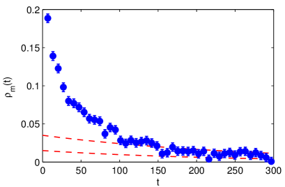
One may object immediately that it is very difficult, if not impossible, to estimate $\tau_{\mathrm{exp}}$, which is needed in the above formulae. In Fig. 1 we therefore just show one numerical result already at this point: the “effective mass plot” from auto-correlation functions of a few observables. Details of the numerical simulation are described only later in Sect. 4.1, however, it is clear from the figure that considering several observables can help for getting a handle on the slow modes.

Figure 1: Effective mass plot $\frac{1}{\tau}\log(\rho_{F}(t)/\rho_{F}(t+\tau))$ for two observables $F$ in run C3d. Here $\tau=6.75$ is the spacing between consecutive measurements.

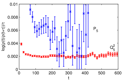
Of course the statistics has to be large enough, but as an empirical observation, an early onset of the plateau in $\log(\rho(t)/\rho(t+\tau))$ is beneficial when $\tau_{\mathrm{exp}}$ is large. Furthermore, the whole proposal relies on the fact the slowest mode, and with it $\tau_{\mathrm{exp}}$, can actually be identified. Absolute certainty on this is virtually impossible to achieve, however, by looking at a large number of operators, at least a significant portion of the relevant space can be covered. Also in case there is an even slower mode than the one identified, the proposed method does provide a more conservative estimate of the contributions up to this threshold, and can therefore improve the analysis.

2.3 Decoupling and dynamical correlation coefficient

Since $\tau_{\mathrm{exp}}$ enters in the exponent in eq. (2.26), this representation is useful if $\tau_{\mathrm{exp}}$ is already known rather precisely – a rare luxury. A more practical representation replaces $\tau_{\mathrm{exp}}$ by an effective one. To this end, we take observables $O_{\beta}$ which couple relatively strongly to the slow MC mode. For QCD possible choices are the square of the topological charge $O_{\beta}=Q^{2}_{\alpha}$ or the smeared plaquette $O_{\beta}=P_{\alpha}$ with $\alpha$ labelling different smearing levels, see Sect. 3.2 for details. We can use

$$\tau_{\mathrm{exp}}^{\mathrm{eff}}(t)=\frac{t}{2\log\left\{\mathrm{Max}_{\beta}{\rho_{\beta}(t/2)\over\rho_{\beta}(t)}\right\}}\,,$$ (2.27)

but clearly other choices are possible. The effective coefficient

$$C_{F}^{\mathrm{eff}}(t)=\rho_{F}(t)\mathrm{e}^{t/\tau_{\mathrm{exp}}^{\mathrm{eff}}(t)}\,.$$ (2.28)

then suggests itself. When detailed balance is guaranteed, a further effective estimator is

$$\widetilde{C}_{F}^{\mathrm{eff}}(t)={[\Gamma_{FG}(t)]^{2}\over\Gamma_{F}(0)\Gamma_{G}(t)}\mathrm{e}^{t/\tau_{\mathrm{exp}}^{\mathrm{eff}}(t)}$$ (2.29)

where $\Gamma_{FG}(t)=\sum_{\alpha,\beta}F_{\alpha}\Gamma_{\alpha\beta}(t)G_{\beta}$ and we have assumed that $G$ is an observable with a strong coupling to the slow mode. In other words $C_{G}$ is large. This representation will be valid (at large $t$) if $\lambda_{1}$ is an isolated eigenvalue and in practice if indeed the critical slowing down is dominated by the single mode $n=1$. It simply follows from the mode decomposition $\Gamma_{FG}(t)=\sum_{n\geq 1}(\lambda_{n})^{t}\;\eta_{n}(F)\eta_{n}(G)$.

Clearly eq. (2.28) is more generic and even expected to be useful when detailed balance is not satisfied, but the advantage of eq. (2.29) is that it can possibly be used at much larger $t$, showing smaller statistical errors in that region.

We can now define what we mean by decoupling of an observable from the slow mode $n=1$: in practice it means $C_{F}\ll 1$ while in terms of critical slowing down, it should be defined as a significant decrease of $C_{F}$ as the correlation length and $\tau_{\mathrm{exp}}$ grow, e.g. $C_{F}\sim(\mathrm{correlation\;length})^{-\gamma}$ with some positive $\gamma$. In MC runs this decoupling is expected to be visible in the behaviour of $\widetilde{C}_{F}^{\mathrm{eff}}(t)$ at moderate time $t$. Given the inherent problems in seeing asymptotic behaviour in numerical simulations, it is useful to go further and define a time scale $\tau_{*}$ through

$$\tau_{\mathrm{exp}}^{\mathrm{eff}}(r\,\tau_{*})=\tau_{*}$$ (2.30)

and

$$C_{F}^{*}(r)=C_{F}^{\mathrm{eff}}(r\tau_{*})\,.$$ (2.31)

In the same way, $C_{F}^{\mathrm{eff}}$ may be replaced by $\widetilde{C}_{F}^{\mathrm{eff}}$. Using $\tau_{*}$ is similar in spirit to the original Sokal proposal for fixing the window of summation for the $\tau_{\mathrm{int}}$ by the point at which the summation window $W$ exceeds a multiple of $\tau_{\mathrm{int}}(W)$. A choice of $r$ significantly smaller than one is necessary when the overall statistics is moderate. We emphasize again our condition eq. (2.22), however. The advantage of eq. (2.31) is that we do not have to consider asymptotically large $t$ with their associated systematics. Decoupling can be studied at a fixed (not unreasonably small) value of $r$. If $C_{F}^{*}(r)$ shows decoupling it will usually also be the case in $C_{F}$.

2.3.1 Relation to static correlations

In the language used here, the square of the standard correlation coefficient of observables $F$ and $G$ is

$$C^{\mathrm{static}}_{FG}={[\Gamma_{FG}(0)]^{2}\over\Gamma_{F}(0)\,\Gamma_{G}(0)}\,.$$ (2.32)

It is a static property, independent of the algorithm as only $t=0$ appears. We now notice that if $G$ “is” approximately the slow mode, which precisely means

$$|\eta_{1}(G)|\gg|\eta_{n}(G)|\;\;\forall\;n>1\,,$$ (2.33)

then we have $\Gamma_{FG}(t)\approx\lambda_{1}^{t}\,\eta_{1}(F)\eta_{1}(G)$ and $\Gamma_{G}(t)\approx\lambda_{1}^{t}\,[\eta_{1}(G)]^{2}$ and therefore also

$$C_{F}\approx C^{\mathrm{static}}_{FG}\,.$$ (2.34)

We may therefore consider $C_{F}$ to be the dynamical correlation coefficient between $F$ and $G$. Generically it will be very different from the static one, emphasizing that the static correlation of the observable $F$ to a slow one (e.g. the topological charge in QCD) is not the proper way to discuss the error of $F$. Rather the dynamical correlation coefficient $C_{F}$ has to be used.

3 Algorithms and observables under study

For the numerical investigation of the HMC and DD-HMC, we now first give the basic definition of the algorithms and then of the observables which we choose to investigate.

3.1 Algorithms

In hybrid Monte Carlo [?] and related algorithms, the gauge fields are updated by solving the classical equations of motion associated with the Hamiltonian

$$H=\frac{1}{2}(\Pi,\Pi)+S(U)\ ,$$ (3.35)

where the antihermitian $\Pi_{x,\mu}$ are the momenta conjugate to the gauge fields $U_{x,\mu}$. Their scalar product is defined as $(\Pi,\Pi)=-2\sum_{x,\mu}\mathrm{tr}\Pi_{x,\mu}^{2}$. With the Monte Carlo time $\tau$, the equations of motion then read

$$\frac{\mathrm{d}}{\mathrm{d}\tau}\Pi_{x,\mu}=-{\mathcal{F}}_{x,\mu}\ \ \text{and}\ \ \frac{\mathrm{d}}{\mathrm{d}\tau}U_{x,\mu}=\Pi_{x,\mu}U_{x,\mu}\ ,$$ (3.36)

where the force ${\mathcal{F}}$ fulfills $(\omega,{\mathcal{F}})=\delta_{\omega}S(U)$ for infinitesimal variations of the gauge field $\delta_{\omega}U_{x,\mu}=\omega_{x,\mu}U_{x,\mu}$. In these definitions, we follow the ones used in the context of the DD-HMC[?]. We give them, because they fix the normalization of the trajectory length $\tau$, which is not unique in the literature. The conventions of Ref. [?] used, e.g., in the MILC code result in a different normalization: a trajectory of length $\sqrt{2}$ in the conventions above corresponds to a unit length trajectory in those of Ref. [?].

The difference between HMC and DD-HMC is that the latter introduces a decomposition of the lattice into blocks of size $B_{0}\times B_{1}\times B_{2}\times B_{3}$. During each trajectory, only the links are updated, which have at least one endpoint in the interior. The fraction of these “active” links is given by

$$R=\frac{\prod_{i=0}^{3}(B_{i}-2)+\frac{1}{4}\sum_{i=0}^{3}\prod_{j\neq i}(B_{j}-2)}{\prod_{i=0}^{3}B_{i}}\ .$$ (3.37)

Since the active links are treated in exactly the same way as in HMC, naively, auto-correlation times will be proportional to the inverse of $R$. Therefore, we scale them in the following by this ratio, noting that in pure gauge theory also the cost of the simulation scales accordingly.

At the end of each trajectory, the HMC algorithm has a global Metropolis acceptance step to correct for the errors in the numerical integration of the equations of motion. For the DD-HMC in pure gauge theory with the Wilson gauge action, however, the molecular dynamics evolution of the active links on each block is independent of the other blocks. We can therefore perform the Metropolis step for each block individually. Compared to the conventional global acceptance step, a given acceptance rate can be achieved with a significantly larger step size. All our runs are done at acceptance rates above $90\%$, and in this case, the block-wise acceptance does not influence the auto-correlation times of the pure gauge observables within errors.

In order to be ergodic, all links of the lattice have to become active within some (composite) series of update steps. This is achieved by translating the domain decomposition relative to the lattice between trajectories. The scheme is described in detail in Ref. [?] and alternates random shifts with directed ones, the latter to increase the efficiency of this step. Because of the directed shifts, however, the full algorithm does not obey detailed balance. Even if eq. (LABEL:e:uppbound) can then not be shown mathematically, we still expect it to be valid at not too small $t$. In any case eq. (2.24) represents a useful estimate of the integrated auto-correlation time. The same reasoning holds true for the factorization behind eq. (2.29).

3.2 Observables

We want to study the effect of the critical slowing down of the (DD)-HMC algorithm on observables of interest for physics. We consider meson two-point functions, Wilson loops and the topological charge, which we will now define. In order to be more sensitive to the slow modes, we also computed some observables on smoothed gauge fields. For this purpose we apply up to five levels of HYP smearing[?] to the link variables.

The slow evolution is very prominent in the topological charge, for which we use the naive gauge definition

$$Q_{\alpha}=\frac{1}{16\pi^{2}}a^{4}\sum_{x,\mu,\nu}\,{\rm tr}\left[F_{\mu\nu}^{(\alpha)}(x)\tilde{F}_{\mu\nu}^{(\alpha)}(x)\right]\ ,$$ (3.38)

where the lattice field strength tensor $F^{(\alpha)}_{\mu\nu}(x)$ is constructed from the clover leaf representation (see e.g. [?] for a definition) but from $\alpha$ times HYP smeared links, where we consider $\alpha\leq 5$. We find little difference beyond the first iteration of smearing.

As physics oriented observables, we compute $W_{1}(l_{1},l_{2})$, the Wilson loops of size $l_{1}\times l_{2}$ after one level of HYP smearing, and the ones without smearing $W(l_{1},l_{2})$. Only the plaquette $P_{\alpha}=W_{\alpha}(a,a)$ is also considered with higher levels of smearing, $\alpha\leq 5$.

In order to study the effects of the slow modes on hadronic observables, we take as an example the correlators used in the quenched study of the $D_{s}$ meson at parameters of Ref. [?]. We compute

$$\begin{split}C_{\mathrm{PP}}(t)&=a^{3}\sum_{\vec{x}}\langle P^{rs}(t,\vec{x})P^{sr}(0,0)\rangle\\ C_{\mathrm{AP}}(t)&=a^{3}\sum_{\vec{x}}\langle A_{0}^{rs}(t,\vec{x})P^{sr}(0,0)\rangle\end{split}$$ (3.39)

with the pseudo-scalar density $P^{rs}=\bar{r}\gamma_{5}s$ and the time component of the axial-vector current $A_{0}^{rs}=\bar{r}\gamma_{0}\gamma_{5}s$. These are estimated on each configuration using the one-end method[?,?] with 5 stochastic $U(1)$ sources per configuration. Interesting observables are the effective meson mass $m_{\mathrm{eff}}$, which is defined through

$$\frac{C_{\mathrm{PP}}(t+a)}{C_{\mathrm{PP}}(t-a)}=\frac{\cosh((t+a-T/2)m_{\mathrm{eff}}(t))}{\cosh((t-a-T/2)m_{\mathrm{eff}}(t))}$$ (3.40)

and the PCAC quark mass ($\partial_{t}f(t)=\frac{1}{a}(f(t+a)-f(t))\,,\;\partial_{t}^{*}f(t)=\frac{1}{a}(f(t)-f(t-a))$)

$$m=\frac{\frac{1}{2}(\partial_{t}+\partial_{t}^{*})C_{\mathrm{AP}}(t)+a\,c_{\mathrm{A}}\,\partial_{t}^{*}\partial_{t}C_{\mathrm{PP}}(t)}{2\,C_{\mathrm{PP}}(t)}\ .$$

For both masses, as well as for the decay constant,

$$f_{\mathrm{PS}}(t)=\frac{C_{\mathrm{AP}}(t)}{[C_{\mathrm{PP}}(t)\,m_{\mathrm{eff}}(t)]^{1/2}}\mathrm{e}^{t\;m_{\mathrm{eff}}(t)/2}\,,$$ (3.41)

we average over a suitably chosen plateau in $t$.

TAG	$\;\;\beta$	$L/a$	$T/a$	$a$[fm]	block	$~{}~{}R$	$\;\tau$	$\;\Delta\tau$	A	stat
A1a	5.789	16	16	0.140	$8^{4}$	0.369	0.5	0.01	0.961	105280
A1b	5.789	16	16	0.140	$8^{4}$	0.369	1	0.01	0.971	70080
A1d	5.789	16	16	0.140	$8^{4}$	0.369	4	0.01	0.968	141120
B0a	6	24	24	0.093	HMC	1	0.5	0.0077	0.931	199600
B0b	6	24	24	0.093	HMC	1	1	0.0077	0.954	110000
B0c	6	24	24	0.093	HMC	1	2	0.0077	0.943	210000
B0d	6	24	24	0.093	HMC	1	4	0.0077	0.946	130000
B0e	6	24	24	0.093	HMC	1	8	0.0077	0.945	116000
B1a	6	24	24	0.093	$12^{4}$	0.53	0.5	0.0077	0.932	52640
B1b	6	24	24	0.093	$12^{4}$	0.53	1	0.0077	0.951	55520
B1c	6	24	24	0.093	$12^{4}$	0.53	2	0.0077	0.945	61280
B1d	6	24	24	0.093	$12^{4}$	0.53	4	0.0077	0.945	65440
B2a	6	24	24	0.093	$12^{2}\times 6^{2}$	0.363	0.5	0.0077	0.945	113800
B2b	6	24	24	0.093	$12^{2}\times 6^{2}$	0.363	1	0.0077	0.958	116400
B2c	6	24	24	0.093	$12^{2}\times 6^{2}$	0.363	2	0.0077	0.956	119200
B2d	6	24	24	0.093	$12^{2}\times 6^{2}$	0.363	4	0.0077	0.954	110400
B3a	6	24	24	0.093	$6^{4}$	0.247	0.5	0.0077	0.956	61000
B3b	6	24	24	0.093	$6^{4}$	0.247	1	0.0077	0.966	128000
B3c	6	24	24	0.093	$6^{4}$	0.247	2	0.0077	0.963	138000
B3d	6	24	24	0.093	$6^{4}$	0.247	4	0.0077	0.962	147000
B4a	6	24	24	0.093	$12\times 6^{3}$	0.3	0.5	0.019∗	0.97	1008000
B4b	6	24	24	0.093	$12\times 6^{3}$	0.3	1	0.02∗	0.97	1584000
B4c	6	24	24	0.093	$12\times 6^{3}$	0.3	2	0.02∗	0.98	780000
C1d	6.136	32	64	0.075	$16\times 8^{3}$	0.422	4	0.02∗	0.946	175360
C2b	6.179	32	32	0.070	$8^{4}$	0.369	1	0.0059	0.956	393000
C2d	6.179	32	32	0.070	$8^{4}$	0.369	4	0.0222∗	0.956	1568160
C3d	6.179	48	48	0.070	$12^{4}$	0.53	4	0.0182∗	0.919	486560
C4d	6.2	32	64	0.068	$16\times 8^{3}$	0.422	4	0.0229∗	0.928	684000
D1d	6.475	48	48	0.047	$12^{4}$	0.53	4	0.0167∗	0.927	707680

Table 1: Parameters of our runs. We give the bare coupling, the size of the lattice, the lattice spacing from $r_{0}=0.5$ fm, the block decompostion in the DD-HMC, the corresponding fraction of active links $R$, the trajectory length $\tau$ and the step size of the integration $\Delta\tau$ along with the acceptance rate $A$ and the total statistics in molecular dynamics units. Runs with blockwise acceptance step are marked with an asterisk on the step size.

4 Results

We have performed a considerable number of long simulations allowing for a study of the dependence of auto-correlations on several parameters. Table 1 presents an overview of the pure gauge theory simulations; on C1 and C4 also quenched measurements were carried out. Most ensembles are lattices generated with the Wilson gauge action of constant volume $L^{4}$ with $L=2.2\,$fm, where the physical scale comes from $r_{0}/a$ of [?] with a nominal value of $r_{0}=0.5\,$fm[?]. We complement this in Sect. 4.5 by a comparison to dynamical $N_{f}=2$ QCD runs.

4.1 Pure gauge theory

Let us start the discussion of the results with the pure gauge ensembles of the Wilson gauge action at constant physical volume, with main interest on the dynamical critical slowing down of the topological charge and how it is reflected in other observables. Since we are in pure gauge theory, the Wilson loops will serve as prime reference.

Figure 2: Normalized auto-correlation function of $Q_{1}^{2}$ at various lattice spacings. The Monte Carlo time is given in molecular dynamics units multiplied by $R$.

4.1.1 Lattice spacing dependence

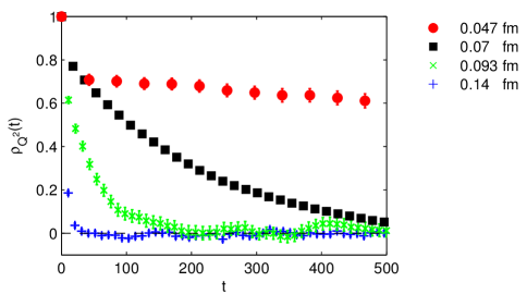
The critical slowing down in the square of the topological charge is rather dramatic as demonstrated in Fig. 2, where we show the normalized auto-correlation function for our four lattice spacings, all with trajectory length $\tau=4$. The Monte Carlo time $t$ is given in molecular dynamics units (MDU) multiplied by $R$. This unit is applied throughout this paper.

From our data we also determine the integrated auto-correlation times by using the criterion given in Eq. (2.11), where we used the default value $S=1.5$ unless specified differently. Results for the plaquette, charge and the square of the charge as well as auto-correlation times are shown in Table 2. Note that the average of the charge is compatible with zero in our long runs, which is an indication that the determination of uncertainties and auto-correlations is under control. We also observe a considerable difference between $\tau_{\mathrm{int}}(Q)$ and $\tau_{\mathrm{int}}(Q^{2})$, in line with the arguments given at the end of section 2.1.

Figure 3: Auto-correlation time of square Wilson loops as a function of their size, for simulation C2d. Smeared loops $W_{1}(r,r)$ are marked as x, while + symobols show $W(r,r)$. The line at the bottom shows ${\tau N_{m}R\over 2}$, where $N_{m}$ is the number of trajectories of length $\tau$ between two consecutives measurements.

TAG	$\langle P\rangle\quad$	$\tau_{\mathrm{int}}(P_{5})$	$\langle Q_{5}\rangle$	$\tau_{\mathrm{int}}(Q_{5})$	$\langle Q^{2}_{5}\rangle$	$\tau_{\mathrm{int}}(Q^{2}_{5})$	$\tau_{*}$
A1a	1.697388(57)	63(15)	-0.05(17)	32(006)	16.8(8)	18(03)	59(07)
A1b	1.697473(56)	32(07)	0.19(15)	19(003)	16.0(5)	8(01)	34(03)
A1d	1.697509(55)	30(05)	0.11(9)	13(001)	16.8(4)	5.9(5)	25(02)
B0a	1.781044(06)	104(16)	-0.68(22)	278(062)	18.3(9)	128(21)	145(12)
B0b	1.781033(07)	56(08)	-0.23(20)	118(024)	19.4(1.0)	71(12)	62(04)
B0c	1.781050(06)	38(04)	-0.07(14)	107(016)	19.3(6)	51(05)	49(03)
B0d	1.781049(09)	32(03)	-0.14(16)	87(014)	18.7(6)	33(04)	44(02)
B0e	1.781053(14)	27(03)	0.02(15)	74(012)	18.7(7)	38(05)	41(03)
B1a	1.781053(13)	109(36)	0.83(52)	214(088)	18.5(1.8)	84(25)	104(18)
B1b	1.781045(13)	42(10)	0.52(43)	148(053)	19.1(1.6)	49(12)	68(10)
B1c	1.781055(16)	44(10)	0.22(33)	100(030)	18.3(1.4)	43(09)	53(07)
B1d	1.781064(21)	46(10)	-0.12(33)	110(033)	17.7(1.3)	43(09)	50(07)
B2a	1.781032(13)	120(35)	-0.41(44)	212(076)	18.6(1.6)	78(19)	107(17)
B2b	1.781066(10)	63(14)	-0.53(41)	186(063)	19.0(1.3)	51(11)	75(10)
B2c	1.781067(13)	44(09)	0.13(32)	111(031)	20.2(1.4)	51(11)	61(08)
B2d	1.781049(17)	30(05)	-0.15(27)	80(021)	18.2(1.0)	34(06)	41(04)
B3a	1.781072(18)	79(29)	0.88(72)	233(118)	17.5(2.1)	58(19)	84(17)
B3b	1.781057(12)	48(11)	-0.10(39)	132(044)	17.8(1.5)	61(15)	71(11)
B3c	1.781039(17)	54(13)	0.05(41)	156(054)	18.2(1.3)	45(10)	57(09)
B3d	1.781033(21)	57(13)	-0.04(32)	105(031)	17.7(1.3)	48(11)	51(06)
B4a	1.781052(05)	97(12)	-0.30(18)	243(043)	19.2(7)	114(15)	135(09)
B4b	1.781049(04)	62(05)	-0.09(10)	131(015)	18.2(4)	56(04)	70(03)
B4c	1.781055(06)	37(03)	-0.24(11)	77(010)	19.5(6)	52(05)	53(02)
C1d	1.822828(04)	42(07)	0.69(61)	281(091)	49.6(4.1)	149(38)	140(18)
C2b	1.835106(02)	80(12)	-0.47(38)	574(189)	18.1(1.6)	248(60)	376(50)
C2d	1.835106(07)	42(07)	-1.16(49)	428(176)	17.2(1.8)	178(54)	159(23)
C4d	1.840897(02)	40(03)	-0.03(34)	503(122)	32.9(1.8)	217(38)	249(20)
D1d	1.909347(02)	55(05)	0.90(65)	4430(2079)	18.8(2.7)	2453(959)	2625(563)

Table 2: The average plaquette, the topological charge and its square along with auto-correlation times (computed with $S=3$) of the smeared plaquette and the (squared) charge for our ensembles described in Table 1. The last column gives the exponential auto-correlation time as defined in Eq. (2.30).

Figure 4: Auto-correlation time of $Q_{5}^{2}$ and the $(0.5~{}{\rm fm})\times(0.5~{}{\rm fm})$ square Wilson loop as a function of the lattice spacing using the DD-HMC algorithm. For $Q_{5}^{2}$ the two curves are fits through the last three points of the two ansätze of Eq. (4.42). For the Wilson loop only the fit to the power law has been performed, through all points.

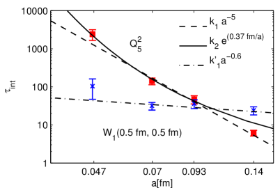
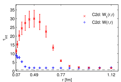
The main result of this section is shown in Fig. 4, where we give the auto-correlation times of $Q_{5}^{2}$ and of $W_{1}(0.5~{}{\rm fm},0.5~{}{\rm fm})$ as a function of the lattice spacing. This Wilson loop is chosen since it is roughly at this size that we find the longest auto-correlation times, see Fig. 3; Creutz ratios behave very similarly. The observed maximum of $\tau_{\mathrm{int}}$ is surprising at first sight, but large Wilson loops are dominated by strong ultraviolet (UV) fluctuations and therefore have a large variance $\Gamma(0)$ compared to their expectation value. In Sect. 4.3 we will consider other long distance observables with a smaller variance.

We compare two ansätze to describe the behaviour of the auto-correlation times,

$$\tau_{\mathrm{int}}(F)=k_{1}\,(a/r_{0})^{z}\qquad\text{and}\qquad\tau_{\mathrm{int}}(F)=k_{2}\,\exp(\alpha/a)$$ (4.42)

where the first is the standard behavior in the vicinity of a continuous phase transition, whereas the exponential form was advocated in the context of the $CP^{(N-1)}$ model in Ref. [?]; we use it only for the topological charge. Even our high statistics data is not precise enough to accurately determine an effective critical exponent. However, with the power law, we get $z\approx 5$ for $Q_{5}^{2}$, a very severe critical slowing down. The data is also not good enough to distinguish it from the exponential form, for which we find $\alpha\approx 0.4$fm. The Wilson loop, on the other hand, follows a power law with $z\approx 0.6$ within our range of data, which is a surprisingly mild behavior. This already demonstrates the decoupling discussed in Sect. 2. The Wilson loops decouple from the slow modes which couple strongly to the square of the charge. We will come back to this subject below. The exponent for the Wilson loops is compatible with the $z=1$ for HMC in free field theory[?].

Figure 5: Auto-correlation time of $Q_{5}^{2}$ in units of molecular dynamics time scaled by $R$ as a function of the trajectory length for the $24^{4}$ lattices at $\beta=6.0$. We show the data for two block decompositions in the DD-HMC as well as data for HMC simulations. The curve is a fit through all points to the functional form $c_{1}/\sqrt{\tau}+\tau/2$.

4.1.2 Dependence on trajectory length and block size

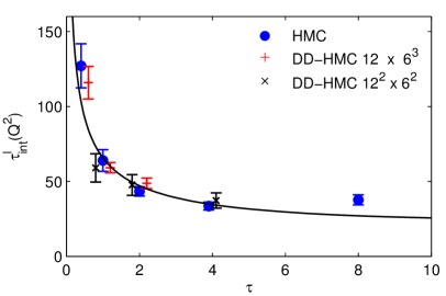
This brings us to the discussion of the various parameters, on which this picture might depend: the trajectory length, the block decomposition and the physical volume. The dependence of $\tau_{\mathrm{int}}(Q_{5}^{2})$ on the trajectory length is visualized in Fig. 5 for the $a\approx 0.1$fm lattices. It demonstrates that longer trajectories can lead to shorter auto-correlation times in units of molecular dynamics time, which takes into account the additional effort needed for the longer trajectories. That longer trajectories can improve the performance of the algorithm has been part of the original motivation for the Hybrid Molecular Dynamics[?], and has since been demonstrated, e.g., in Ref. [?]. In free field theory it is known that the optimal trajectory length depends on the observable and typically increases when the correlation length increases [?]. As long as the system is in a regime with $\tau_{\mathrm{int}}\gg\tau$, one can argue that the momentum refreshment at the beginning of each trajectory initiates a random change of direction in the otherwise directed walk. One then expects longer trajectories to decrease $\tau_{\mathrm{int}}$ proportional to $1/\sqrt{\tau}$, but at most down to the smallest possible value of $\tau_{\mathrm{int}}=\tau/2$, which means $\tau_{\mathrm{int}}=1/2$ in units of complete updates. This simple model describes the gross features of our data reasonably well. Also on the finer C lattices, given in Table 2, the corresponding improvement can be observed.

The data of the figure are also collected in Table 2 together with those from different block decompositions and also from the HMC algorithm. We observe that the blocks do not have a measureable impact on the auto-correlation times beyond the simple rescaling with the active link ratio $R$. Of course, the blocks have to have a reasonable minimal size. Our smallest blocks are still at least 0.5fm across, which is around the pure gauge theory correlation length defined from the string tension.

4.1.3 Dependence on volume and discretization

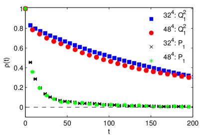
Most of our ensembles have a constant physical volume with $L=2.2$fm, for which finite size effects of typical equilibrium expectation values are known to be small in the pure gauge theory. In order to check for a potential $L$-dependence of auto-correlations, we also generated an $L=3.3$ fm ensemble at $\beta=6.18$. Figure 6 demonstrates that no significant volume dependence is present – neither for the smeared plaquette $P_{1}$ nor for the squared charge $Q_{1}^{2}$.

Figure 6: Auto-correlation time of $Q_{1}^{2}$ and the smeared plaquette $P_{1}$ at $\beta=6.18$ on a $32^{4}$ and a $48^{4}$ lattice.

The emerging picture might also depend on the particular discretization used. So far, all results were for the Wilson gauge action. Therefore, we also generated an ensemble with the Iwasaki action with $a=0.09$fm, with the same volume and simulation parameters, using the HMC algorithm in both cases. We observe a drastically larger auto-correlation time for the topological charge,

$$\tau_{\mathrm{int}}(Q_{5}^{2})=\phantom{0}34(\phantom{0}4) \text{for Wilson gauge action},$$ (4.43)

$$\tau_{\mathrm{int}}(Q_{5}^{2})=220(50)$$ for Iwasaki gauge action (4.44)

However, this is not replicated in other observables, both the plaquette and the smeared plaquette having roughly the same auto-correlation times for the two actions.

4.2 The charge in subvolumes

Ultimately one needs to find an algorithm with smaller auto-correlations. For this purpose it is important to understand more about how the HMC moves the gauge fields through configuration space. Of course this is a difficult problem, as we need to reformulate it in terms of specific (gauge invariant) observables.

An interesting such question is whether topological charge is being moved from some space-time volume to another one more quickly than the total charge is changing. This can be looked at by restricting the sum in eq. (3.38) to a region ${\cal R}$, computing the charge inside that region

$$Q_{\alpha}^{\cal R}=\frac{1}{16\pi^{2}}a^{4}\sum_{x\in{\cal R}}\sum_{\mu,\nu}\,{\rm tr}\left[F_{\mu\nu}^{(\alpha)}(x)\tilde{F}_{\mu\nu}^{(\alpha)}(x)\right]\ .$$ (4.45)

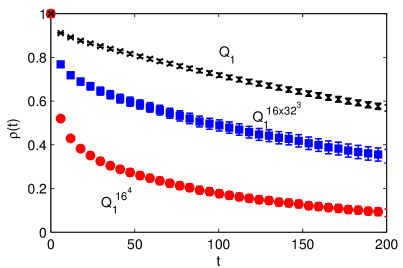
Its MC history will show whether charge has flown in or out of the region. More quantitatively we can directly look at the auto-correlation function of $Q_{\alpha}^{\cal R}$ as shown in Fig. 7. The subvolume charge does decorrelate significantly faster than the total charge, but there is still a quite significant coupling to the slow mode remaining. The decoupling coefficient $C^{*}$ is around $0.7$ for the $16\times 32$ sublattice and about $C^{*}=0.15$ for the $16^{4}$ subvolume. The latter is a significant suppression.

Figure 7: Auto-correlation function of $Q_{1}^{\cal R}$, with ${\cal R}$ being the full lattice, half the lattice (cut in one dimension) and a 16th of the lattice, cut in half in all dimensions. We used a sequence of 320000 MDU of the C2d run.

4.3 Quenched approximation

Figure 8: Auto-correlation function of the mass of the $c\,\bar{c}^{\prime}$ pseudo-scalar meson with $m_{c}=m_{c^{\prime}}=m_{\mathrm{charm}}$. The meson mass is obtained from a plateau average. The two dashed lines show the upper/lower bound region of the tail contribution to the normalized auto-correlation function, given by $C^{*}_{F}\;e^{-t/\tau_{*}}$.

Considering phenomenological applications and access to different QCD observables, hadron correlation functions are more interesting observables than Wilson loops. In order to have very good statistics and observables which do not suffer from an intrinsically large variance, we study pseudo-scalar correlation functions. For cost reasons this is done just on $64\times 32^{3}$ lattices. As an example we perform a study similar to the one in Ref. [?], where the mass and decay constant of the $D_{s}$ as well as the charm quark mass were investigated in the quenched approximation. Neglecting sea quark effects allows us to generate an ensemble with the high statistics necessary for detecting even small influences of the slow modes. However, it comes at the price that small quark masses are not possible without running into the problem of exceptional configurations[?]. Even at the mass of the strange quark which we take over from Ref. [?], we observed at least one clearly exceptional strange quark propagator in 40000 measurements. We discard suspicious configurations using the criterion that the fourth moment of the strange pseudo-scalar correlator $M_{4}$ with $M_{n}=a\sum_{t=-T/2+a}^{T/2-a}t^{n}C_{PP}(t)$ is at least ten standard deviations away from the average value.

We used the Wilson gauge action at $\beta=6.2$ on a $64\times 32^{3}$ lattice, see also Table 1, simulation C4d. The Wilson fermion action is non-perturbatively $\mathrm{O}(a)$ improved [?] and we chose hopping parameters[?] $\kappa_{\mathrm{strange}}=0.134959$ and $\kappa_{\mathrm{charm}}=0.124637$. The quark fields are anti-periodic in time.

The large statistics allows us to accurately measure the auto-correlation function. In Figure 8 we show the example of the meson mass with the longest auto-correlation among those considered in this study: the pseudo-scalar $c\bar{c}^{\prime}$ meson with $m_{c^{\prime}}=m_{c}=m_{\mathrm{charm}}$. The normalized auto-correlation function quickly falls to $\rho(6)\approx 0.2$, but then exhibits a long tail for which we get non-zero values up to $t\approx 200$. As will be discussed further in Sect. 4.4, the contribution of the slow mode to $\tau_{\mathrm{int}}$ is $C_{F}\tau_{\mathrm{exp}}\approx 50\%$.

Observable	$\tau_{\mathrm{int}}^{\mathrm{l}}(S=1.5)$	$\tau_{\mathrm{int}}^{\mathrm{l}}(S=3)$	$\tau_{\mathrm{int}}^{\mathrm{u}}$
$m_{\mathrm{PS}}^{ss^{\prime}}$	6.9(2)	8.5(4)	11(1)
$f_{\mathrm{PS}}^{ss^{\prime}}$	3.9(1)	4.0(1)	7(1)
$m^{ss^{\prime}}$	3.7(1)	3.7(1)	7(1)
$m_{\mathrm{PS}}^{cc^{\prime}}$	11.0(4)	13.3(7)	15(2)
$f_{\mathrm{PS}}^{cc^{\prime}}$	4.3(1)	5.0(2)	8(1)
$m^{cc^{\prime}}$	5.6(1)	6.6(3)	9.4(1)
$Q^{2}_{1}$	183(21)	191(31)	196(14)
$P_{1}$	12.0(4)	13.5(7)	15(2)
$W_{1}(0.5\mathrm{fm},0.5\mathrm{fm})$	27(3)	30(5)	34(5)

Table 3: Auto-correlation times for the quenched strange and charm quark observables along with pure gauge observables on the C4 lattice and Wilson loop on the C2 lattice. The window $W_{l}$ has been obtained by setting the $S$ parameter in eq. (2.10) equal to $1.5$ and $3$. Larger values of $S$ correspond to larger windows.

Other results are shown in Table 3. The important observation on this table is that the auto-correlation times for all observables $F$ that we looked at are $\tau_{\mathrm{int}}(F)\lesssim 20$ except for the squared topological charge, for which we find $\tau_{\mathrm{int}}(Q_{1}^{2})\approx\tau_{\mathrm{int}}(Q_{5}^{2})\approx 200$. Thus there is very good evidence that the effect of the slow mode, which is clearly visible in the charge, is strongly supressed in other observables. Still this supression should be verified for each new observable and the effect of the slow mode should be estimated. The different numbers for the $\tau_{\mathrm{int}}$-estimates in the table illustrate that significant contributions by slow modes are present. We now turn to this issue of good error estimates.

4.4 Improved error estimates

Figure 9: The coefficient $C_{F}^{*}(r)$, eq. (2.31), for $F$ the squared, once smeared Wilson loop of size 0.5fm$\times$0.5fm. Four different lattice spacings are shown in the pure gauge theory, from top to bottom: A1d, B3d, C2d, D1d.

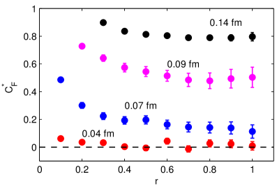
Our results of the previous two subsections call for improved error estimates (Sect. 2.2) where the contribution of a long tail of the auto-correlation functions is included. We discuss numerical results from both the pure gauge theory runs and the quenched run. Also the decoupling of Sect. 2.3 is demonstrated for these cases.

In the pure gauge theory data we clearly see decoupling of the Wilson loops. Recall from Fig. 3 that the maximum auto-correlation is present for the once-smeared 0.5fm$\times$0.5fm Wilson loop. In Fig. 9 we thus show $C_{W_{1}}^{*}(r)$ introduced in Eq. (2.31) for that size. The dependence on $r$ (not to be confused with the size of the loop) is rather insignificant, while the plot shows how the amplitude $C_{W_{1}}^{*}(r)$ decreases at smaller lattice spacings, independent of any small residual variation with $r$.

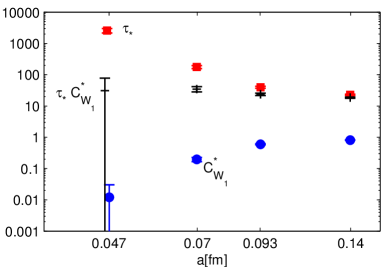
The contribution of the slowest mode to $\tau_{\mathrm{int}}$ is given by the product $\tau_{\mathrm{exp}}\,C_{W_{1}}$. In order to analyse the critical behavior of this quantity we fix $r=0.5$ and plot $\tau_{*}$, our estimator for $\tau_{\mathrm{exp}}$, the coefficient $C_{W_{1}}^{*}(0.5)$ as well as the combination $\tau_{*}\,C^{*}_{W_{1}}$ against the lattice spacing in Fig. 10. We see the strong critical slowing down as an increase of $\tau_{*}$ by orders of magnitude, which is, however, basically compensated by the decoupling characterized by the critical behavior of $C_{W_{1}}^{*}(0.5)$. As a result, the contribution of the slow mode to the auto-correlation time of the Wilson loop stays small and no severe critical slowing down is observed in this quantity.

Figure 10: The slow mode contribution $\tau_{\mathrm{exp}}\,C_{F}^{*}(r)$, eq. (2.31), for $F$ the squared, once smeared Wilson loop of size 0.5fm$\times$0.5fm as a function of the lattice spacing.

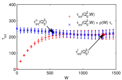
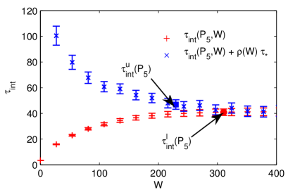
We now turn again to pseudo-scalar correlation functions on the C4d lattice. We saw earlier that the largest auto-correlation is seen for the correlator of two distinct flavor but mass-degenerate quarks with the mass of the charm quark. Therefore we illustrate the statements made in Sect. 2.2 for this example as well as for the squared topological charge. The estimate of $\tau_{\mathrm{exp}}$ to be inserted into eq. (2.24) and eq. (2.25) was already discussed in Sect. 2.2. Here we show eq. (2.24) in comparison to eq. (2.23) as a function of the window size $W_{\mathrm{u}},W_{\mathrm{l}}$. They are plotted together in Fig. 11. We see that $\tau_{\mathrm{int}}^{\mathrm{u}}(P_{5})$ represents a much safer estimate of $\tau_{\mathrm{int}}$ than $\tau_{\mathrm{int}}^{\mathrm{l}}$, also at a somewhat small value of $W_{\mathrm{u}}$, which one might be forced to choose if the statistics is small. In the case of the topological charge squared, the auto-correlation function follows closely a single exponential decay already at rather small times. Hence the determination of $\tau_{\mathrm{int}}$ including the tail from eq. (2.24) is precise at values of $W_{\mathrm{u}}$ which are much smaller than the one that is chosen by our criterion in Sect. 2.2.

Figure 11: Top: The error estimates $\tau_{\mathrm{int}}^{\mathrm{l}}(Q_{5}^{2})$ and $\tau_{\mathrm{int}}^{\mathrm{u}}(Q_{5}^{2})$ according to Eqs. (2.23) and (2.24) as a function of the respective window $W_{l/u}$. Their values according to our prescription are indicated by the filled symbol points. Bottom: the same for $P_{5}$.

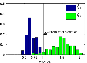
The safer error estimate described in Sect. 2.2 is convincing in the case of a large statistics – on the C4d lattice the total statistics is around $1000\times\tau_{\mathrm{exp}}$. For significantly smaller sample sizes the error estimate will of course be less reliable. We tested the stability by dividing the total run into pieces of about $2500\,(\mathrm{MDU}\cdot R)$ each, which is about $10\tau_{\mathrm{exp}}$. The histograms in Fig. 12 show the distribution of both standard and the improved error estimate following exactly Sect. 2.2. The observable is again the $c\bar{c}^{\prime}$ pseudo-scalar mass. These distributions teach the following lesson. The improved error estimate of eq. (2.24) and eq. (2.25) is always safely close to the true error or somewhat above it, while eq. (2.23) with the standard window size typically underestimates the error – not so rarely by a factor two. An error estimate using $\tau_{\mathrm{int}}^{\mathrm{u}}$ is recommended. The histograms also remind us of an obvious fact: typically the error of the statistical error is not that small in QCD simulations.

Figure 12: Histogram distribution of the error bars (upper and lower bound) for the mass of the pseudo-scalar $\bar{c}\gamma_{5}c^{\prime}$. The central dashed lines show the error of the error from the total statistics.

4.5 Full QCD

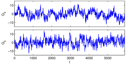
As part of the CLS effort, we have carried out two rather long $N_{\mathrm{f}}=2$ QCD runs with about 16000 MDU each, and with $R=0.37$. The ensemble E5f is generated with $\tau=1/2$ and E5g has $\tau=4$. Both simulations describe the same physics, using the non-perturbatively $\mathrm{O}(a)$ improved action[?] at $\beta=5.3\,,\,\kappa=0.13625$ on $64\times 32^{3}$ lattices. The lattice spacing is read off from $r_{0}/a\approx 7$ [?] and we are close to $m_{\pi}r_{0}=1$, which means a pion mass of around 400 MeV. We will compare directly to the C1 lattice whose lattice spacing is matched to this value of $r_{0}/a$. But first we illustrate the quality of the runs by some time histories in Fig. 13: the runs contain many sign-flips of the topological charge. As expected the frequency of topology changes is better for the lower, $\tau=4$, run than for the upper, $\tau=1/2$, case.

Figure 13: Histories of the charge $Q_{5}$ in simulations E5f with $\tau=0.5$ (top) and E5g with $\tau=4$ (bottom). The Monte Carlo time $t$ is given in molecular dynamics time units.

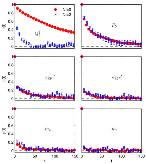
A one-to-one comparison of the auto-correlation functions, quenched vs. $N_{\mathrm{f}}=2$, is presented in Fig. 14. One observes a very similar decorrelation of all observables quenched and in full QCD, except for the squared topological charge which decorrelates much faster with dynamical fermions. Unfortunately we cannot offer a real theoretical understanding of this rather striking observation. However, note that the change of the gauge action (in the pure gauge theory) from Wilson plaquette action to Iwasaki action has a similar effect, namely the auto-correlations of $Q^{2}$ were strongly affected while auto-correlations of other observables are essentially unchanged. Among the effects of the introduction of the fermion determinant is a change of the effective gauge action in the ultraviolet. Beyond the leading $\beta$-shift there are also dimension six terms and this “part” of the fermion determinant is the same as a change of the lattice gauge action.

As we did for the pure gauge theory, we now come to the extraction of the exponential auto-correlation time, see Fig. 15. The estimator $\tau_{\mathrm{exp}}^{\mathrm{eff}}(t,F)=\frac{t}{2\log\left\{{\rho_{F}(t/2)\over\rho_{F}(t)}\right\}}$ is shown for those observables with the slowest decorrelation out of our set. Clearly the determination of $\tau_{\mathrm{exp}}^{\mathrm{eff}}$ is difficult, but it seems possible. The location of $\tau_{*}$, which we remind the reader is our estimate eq. (2.30) for $\tau_{\mathrm{exp}}$, is indicated in the figure.

Figure 14: Comparison of the normalized auto-correlation function $\rho(t)$ between quenched and dynamical simulations at the same value of $r_{0}/a\sim 7$ for different observables. The data is from the C1d and E5g runs, respectively. Top: Comparison for topological charge squared and plaquette. Center: Pseudo-scalar meson masses with mass-degenerate quarks of the charm quark mass on the left ($\bar{c}\gamma_{5}c^{\prime}$) and strange quark mass on the right ($\bar{s}\gamma_{5}s^{\prime}$), extracted from plateau averages over $x_{0}\in[23a,27a]$. Bottom: Auto-correlation functions of PCAC quark masses at $x_{0}=24a$.

Figure 15: Estimators for the exponential auto-correlation time from smeared plaquette and topological charge in pure gauge (C1d) and dynamical (E5g) simulations.

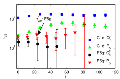
The numbers for $\tau_{\mathrm{int}}$ and $\tau_{*}$ are listed in Table 4. We see again that auto-correlation times for long trajectories with length $\tau=4$ are around a factor two smaller than those for $\tau=1/2$. In the table we list numbers for $\tau_{*}$ determined just from the indicated observable for illustration. In our estimate of $\tau_{\mathrm{int}}^{\mathrm{u}}$ the maximum one is then taken into account as defined in eq. (2.27). The more observables one considers, the better (larger) the estimate of $\tau_{\mathrm{exp}}$ will get. Even if this is still below the true value of $\tau_{\mathrm{exp}}$, it will provide us with a more realistic estimate of $\tau_{\mathrm{int}}$.

4.5.1 Proposal for error estimates

The numbers in Table 4 come from a rather long simulation. Such data is not always available. Here we propose how one may proceed in this situation, using a reasonable estimate of the contribution of the tail of the auto-correlation function. Eq. (2.24) should be used when an onset of a tail is visible in the data and we suggest to choose $W_{\mathrm{u}}$ such that $\delta[\rho_{F}(W_{\mathrm{u}})]\approx\rho_{F}(W_{\mathrm{u}})/3$. On the other hand for auto-correlations which quickly fall off, eq. (2.25) is recommended. With low statistics an estimate of $\tau_{\mathrm{exp}}$, needed for these formulae, is impossible to obtain. We therefore suggest to use a value for a not-so-small $a$ with good statistics together with the scaling observed in the pure gauge theory. For our $\mathrm{O}(a)$-improved action at $N_{\mathrm{f}}=2$ we hence suggest an $a^{-5}\sim\exp(7\beta)$ scaling (see eq.(4.5) of [?]). Together with $\tau_{\mathrm{exp}}\approx 40$ at $\beta=5.3$, this leads for the action of [?] to

$$R\,\tau_{\mathrm{exp}}\approx 200\,\exp(7\,(\beta-5.5))\,\mathrm{MDU}\ .$$ (4.46)

For safety reasons, one may attach an error of a factor 2 to this estimate and should of course be aware of the assumptions made above. The best situation is an observable with a strong decoupling, i.e. a small auto-correlation function $\rho_{F}(W_{\mathrm{u}})$ or $\rho_{F}(W_{0})$, for which the intrinsic uncertainties of the model eq. (4.46) are not that relevant.

	$Q_{5}^{2}$					$P_{5}$
TAG	$\langle Q_{5}^{2}\rangle$	$a^{4}\chi_{\mathrm{t}}$	$\tau_{\mathrm{int}}^{\mathrm{l}}$	$\tau_{\mathrm{int}}^{\mathrm{u}}$	$\tau_{*}$	$\tau_{\mathrm{int}}^{\mathrm{l}}$	$\tau_{\mathrm{int}}^{\mathrm{u}}$	$\tau_{*}$
C1d	50(4)	2.4(2) $\times 10^{-5}$	137(25)	134(15)	140(18)	38(4)	43(5)	74(11)
E5f	17.3(1.8)	0.82(9) $\times 10^{-5}$	16(4)	23(5)	21(5)	84(31)	66(13)	66(19)
E5g	18.9(1.5)	0.90(7) $\times 10^{-5}$	10(2)	14(3)	15(4)	29(8)	29(5)	39(12)

Table 4: Comparison between the integrated auto-correlation times for the topological charge and the smeared plaquette between the dynamical and the corresponding pure gauge ensemble. The dynamical runs E5f and E5g have trajectory length $\tau=0.5$ and $\tau=4$, respectively. The pure gauge run C1d has $\tau=4$. Also the value of the topological susceptibility, $\chi_{\mathrm{t}}$, is given.

5 Summary and conclusions

In this paper we have established a very severe critical slowing down of the topological charge in pure Yang-Mills theory when using the (DD)-HMC algorithm. A dynamical critical exponent of $z=5$ means that, at constant volume, the full simulation scales with $a^{-10}$ at least, since an HMC type algorithm is expected to scale with $a^{-4}$ from the increasing number of lattice points and typically an additional factor of $a^{-1}$ from the decreasing step size. However, we also investigated Wilson loops, which are more commonly in the focus of interest. They are not affected in the same way, exhibiting a much milder slowing down while approaching the continuum limit ($z\approx 0.5\ldots 1$). Martin Lüscher investigated observables after integrating the Wilson flow[?] for some distance which removes UV fluctuations. These observables effectively show $z\approx 2$ [?], a critical slowing down in between $Q^{2}$ and the Wilson loops.

We have also considered observables formed from pseudoscalar correlation functions, both in a quenched setting and for $N_{\mathrm{f}}=2$. These quantities are of immediate interest and at the same time not plagued by large UV fluctuations. At a lattice spacing of $a\approx 0.07$fm their autocorrelation functions are much better behaved than the one of $Q_{5}^{2}$ but a weak coupling to the slow mode is seen in Fig. 14. Unfortunately, a systematic study as a function of the lattice spacing and quark mass is prohibitively expensive, but we expect that these observables continue to couple only weakly to the slow mode and their slowing down is significantly less severe than for the topological charge.

On the one hand, this is encouraging. In practical simulations, unless we are interested in the slow observables themselves, we do not need to gather enough statistics to accurately determine their auto-correlation time. It is sufficient to have a decent sampling in the slow modes to assure practical ergodicity, i.e. a few times their auto-correlation times is needed. On the other hand, the danger remains that there are even slower modes which are so slow that the corresponding fluctuations do not show in the full runtime. The only way to study this is to start simulations in parameter space, which can be considered safe and then move in small steps towards the critical points, monitoring a large number of observables and relying on the continuity of auto-correlations in terms of the system’s parameters.

Even if the coupling to the slow modes may be small it is important for a correct error analysis. We described a practical method to take these effects into account. It relies on the fact that information about $\tau_{\mathrm{exp}}$ can be obtained through observables which couple strongly to the corresponding mode. Under these circumstances, the error analysis can be made significantly safer.

Still, a true solution to the critical slowing down has to be an algorithmic one which at least solves the problem regarding the topological charge. The dramatic progress in the fermion algorithms which the field has witnessed during the last decade gives us hope that this can actually be achieved.

Acknowledgements. We would like to thank M. Lüscher and F. Palombi for many useful discussions and the possibility to use some of their data as well as U. Wolff and other members of CLS for helpful discussions. We are grateful to A. Kennedy for a critical reading of an earlier version of the manuscript. This work is supported by the Deutsche Forschungsgemeinschaft in the SFB/TR 09 and by the European community through EU Contract No. MRTN-CT-2006-035482, “FLAVIAnet”. We thank the John von Neumann institute for computing and the HLRN for allocating computer time for this project. Part of our runs were performed on the PAX cluster at DESY, Zeuthen.

Appendix A Error of the Error

An introduction to the error analysis of correlated data from a Markov chain with references can be found in [?] while the case of functions of the primary observables is treated in [?]. Here we review the main formulae for estimating the error of the error from these references and make those explicit which are not given there.

Our estimator for the mean, eq. (2.2), and the auto-correlation function, eq. (2.4), are

$$\overline{O}_{\alpha} = {1\over N}\sum_{t=1}^{N}O_{\alpha}(q_{t})\;,\quad\overline{O}_{F}=F(\overline{O}_{\alpha})$$ (A.47)

$$\overline{\Gamma}_{FF^{\prime}}(t) = {1\over N-|t|}\sum_{u=1}^{N-|t|}dF(q_{u})d{F^{\prime}}(q_{u+t})+{1\over N^{2}}\sum_{u=1}^{N}dF(q_{u})d{F^{\prime}}(q_{u})\,,$$ (A.48)

where

$$dF(q) = \sum_{\alpha}F_{\alpha}(O_{\alpha}(q)-\overline{O}_{\alpha})$$ (A.49)

which for $\overline{\Gamma}_{FF^{\prime}}$ contains a bias correction discussed in [?]. In the computation of our auto-correlation times, e.g. eq. (2.24), we replace $\Gamma$ by its estimator $\overline{\Gamma}$.

In Sect. 2 we introduced various quantities which are functions $G(\{\Gamma_{F}(t)\})$. Their error is computed from simple error propagation

$$(\delta G)^{2}={1\over N}\sum_{A,B}{\partial G\over\partial\Gamma_{A}}\Sigma_{AB}{\partial G\over\partial\Gamma_{B}}$$ (A.50)

where $A=(F,u)$ and $B=(F^{\prime},v)$ collect the observable and time variable and run over all components of the auto-correlation functions. The covariance matrix $\Sigma_{AB}$ is given by

$$\Sigma_{AB} = {1\over N^{2}}\sum_{s=1}^{N}\sum_{t=1}^{N}dF(q_{s})dF(q_{s+u})d{F^{\prime}}(q_{t})d{F^{\prime}}(q_{t+v})-{\overline{\Gamma}_{F}}(u){\overline{\Gamma}_{F^{\prime}}}(v)\;.$$ (A.51)

Neglecting the completely connected part of the fourth moment in eq. (A.51), we have the approximation

$$\overline{\Sigma}_{AB}\approx{1\over N}\sum_{m=-\infty}^{\infty}\Gamma_{FF^{\prime}}(m+v)\Gamma_{FF^{\prime}}(m+u)+\Gamma_{FF^{\prime}}(m+v)\Gamma_{FF^{\prime}}(m-u)\,,$$ (A.52)

which in practice we evaluate with the cut eq. (A.56) to be discussed below.

In some simple cases, approximations can be applied to eq. (A.50) to derive more compact error formulae, for example [?,?]

$$(\delta{\tau_{\mathrm{int}}(W)})^{2} \approx{2(2W+1)\over N}\tau_{\mathrm{int}}^{2}(W)\;,$$ (A.53)

$$(\delta{\rho(t)})^{2} \approx{1\over N}\sum_{m=1}^{\infty}(\rho(m+t)+\rho(m-t)-2\rho(m)\rho(t))^{2}\,.$$ (A.54)

Furthermore we used the approximation

$$(\delta{\tau_{\mathrm{int}}^{\mathrm{u}}})^{2}\approx(\delta{\tau_{\mathrm{int}}(W_{u})})^{2}+\tau_{\mathrm{exp}}^{2}(\delta{\rho(W_{u})})^{2}+\rho^{2}(W_{u})(\delta{\tau_{\mathrm{exp}}})^{2}\;,$$ (A.55)

for the error of eq. (2.24) after checking that the left out cross terms are negligible. Also in the case of eq. (2.29) a similar approximation has been applied. For all other quantities we remained directly with eq. (A.50).

As mentioned, the evaluation of the sum in eq. (A.52) and also the one in eq. (A.54) require the introduction of a cutoff on the sum over $m$. This can be done with the function

$$\tilde{\Gamma}(x)=\begin{cases}\overline{\Gamma}(x)&|x|\leq W_{\Sigma}\\ 0&|x|>W_{\Sigma}\;.\end{cases}$$ (A.56)

(and $\tilde{\rho}$) where we omit the subscripts to keep notation light. The computation of $\Sigma(u,v)$ is then carried out as the sum of terms $\sum_{m}\tilde{\Gamma}(m)\tilde{\Gamma}(m+t)$ at times $t=u+v$ and $t=u-v$:

$$\overline{\Sigma}(u,v)\approx{1\over N}\sum_{m}\left(\tilde{\Gamma}(m)\tilde{\Gamma}(m+u+v)+\tilde{\Gamma}(m)\tilde{\Gamma}(m+u-v)\right)$$ (A.57)

that can be done in at most $O(W_{\Sigma}^{2})$ operations. The size of $W_{\Sigma}$ can be discussed in similar manner as we have done about window sizes for the auto-correlation function. In our analysis we take $W_{\Sigma}=W$, with $W$ given by prescription eq. (2.11), however, using $W_{\Sigma}=2W$ gives similar results.

In principle one could think about adding a tail contribution to eq. (A.56), but this goes too far, even with the statistics we had at hand.

References

- [1] C. Aubin, (ed. ) et. al., Lattice field theory. Proceedings, 26th International Symposium, Williamsburg, USA, July 14-19, 2008,, PoS LATTICE2008 (2008) 1.
- [2] Lattice field theory. Proceedings, 27th International Symposium, Beijing, China, July 26-31, 2009,, PoS LATTICE2009 (2009) 1.
- [3] L. Del Debbio, H. Panagopoulos, and E. Vicari, Theta dependence of SU(N) gauge theories, JHEP 08 (2002) 044, [hep-th/0204125].
- [4] B. Alles, G. Boyd, M. D’Elia, A. D. Giacomo, and E. Vicari, Hybrid monte carlo and topological modes of full QCD, Physics Letters B 389 (1996), no. 1 107 – 111.
- [5] G. S. Bali, N. Eicker, T. Lippert, H. Neff, B. Orth, K. Schilling, T. Struckmann, and J. Viehoff, Quark mass effects on the topological susceptibility in QCD, Phys. Rev. D 64 (Aug, 2001) 054502.
- [6] C. Bernard et. al., Topological susceptibility with the improved Asqtad action, Phys. Rev. D68 (2003) 114501, [hep-lat/0308019].
- [7] C. Jung, Status of dynamical ensemble generation, arXiv:1001.0941.
- [8] A. D. Sokal, Monte Carlo Methods in Statistical Mechanics: Foundations and New Algorithms, NATO Adv. Sci. Inst. Ser. B Phys. (1997) 131–192.
- [9] N. Madras and A. D. Sokal, The pivot algorithm: A highly efficient Monte Carlo method for the self-avoiding walk, J. Stat. Phys. 50 (1988) 109.
- [10] ALPHA Collaboration, U. Wolff, Monte carlo errors with less errors, Comput. Phys. Commun. 156 (2004) 143–153, [hep-lat/0306017].
- [11] M. Lüscher, Computational Strategies in Lattice QCD, arXiv:1002.4232.
- [12] S. Duane, A. D. Kennedy, B. J. Pendleton, and D. Roweth, Hybrid Monte Carlo, Phys. Lett. B195 (1987) 216–222.
- [13] M. Lüscher, Schwarz-preconditioned HMC algorithm for two-flavour lattice QCD, Comput. Phys. Commun. 165 (2005) 199, [hep-lat/0409106].
- [14] S. A. Gottlieb, W. Liu, D. Toussaint, R. Renken, and R. Sugar, Hybrid Molecular Dynamics Algorithms for the Numerical Simulation of Quantum Chromodynamics, Phys.Rev. D35 (1987) 2531–2542.
- [15] A. Hasenfratz and F. Knechtli, Flavor symmetry and the static potential with hypercubic blocking, Phys. Rev. D64 (2001) 034504, [hep-lat/0103029].
- [16] M. Lüscher, S. Sint, R. Sommer, and P. Weisz, Chiral symmetry and O() improvement in lattice QCD, Nucl. Phys. B478 (1996) 365–400, [hep-lat/9605038].
- [17] J. Heitger and A. Jüttner, Lattice cutoff effects for with improved Wilson fermions - a final lesson from the quenched case, JHEP 05 (2009) 101, [arXiv:0812.2200].
- [18] R. Sommer, Leptonic decays of B and D mesons, Nucl.Phys.Proc.Suppl. 42 (1995) 186–193, [hep-lat/9411024].
- [19] UKQCD Collaboration Collaboration, M. Foster and C. Michael, Quark mass dependence of hadron masses from lattice QCD, Phys.Rev. D59 (1999) 074503, [hep-lat/9810021].
- [20] S. Necco and R. Sommer, The N(f) = 0 heavy quark potential from short to intermediate distances, Nucl. Phys. B622 (2002) 328–346, [http://arXiv.org/abs/hep-lat/0108008].
- [21] R. Sommer, A new way to set the energy scale in lattice gauge theories and its applications to the static force and in SU(2) Yang-Mills theory, Nucl. Phys. B411 (1994) 839, [hep-lat/9310022].
- [22] L. Del Debbio, G. M. Manca, and E. Vicari, Critical slowing down of topological modes, Phys.Lett. B594 (2004) 315–323, [hep-lat/0403001].
- [23] A. D. Kennedy and B. Pendleton, Cost of the generalised hybrid Monte Carlo algorithm for free field theory, Nucl. Phys. B607 (2001) 456–510, [hep-lat/0008020].
- [24] ALPHA Collaboration, H. B. Meyer et. al., Exploring the HMC trajectory-length dependence of autocorrelation times in lattice QCD, Comput. Phys. Commun. 176 (2007) 91–97, [hep-lat/0606004].
- [25] K. Mütter, K. Schilling, R. Sommer, and P. De Forcrand, Towards the limit of the quenched approximation in hadron mass calculations, In *Brookhaven 1986, Proceedings, Lattice Gauge Theory ’86* 257-267. (1986).
- [26] M. Lüscher, S. Sint, R. Sommer, P. Weisz, and U. Wolff, Non-perturbative O() improvement of lattice QCD, Nucl. Phys. B491 (1997) 323–343, [hep-lat/9609035].
- [27] ALPHA Collaboration, K. Jansen and R. Sommer, O() improvement of lattice QCD with two flavors of Wilson quarks, Nucl. Phys. B530 (1998) 185–203, [hep-lat/9803017].
- [28] B. Leder, Scale and the static potential from the CLS lattices, talk at Lattice 2010, Villasimius, Italy (2010).
- [29] M. Della Morte et. al., Preparing for =2 simulations at small lattice spacings, PoS LAT2007 (2007) 255, [arXiv:0710.1263].
- [30] M. Lüscher, Properties and uses of the Wilson flow in lattice QCD, JHEP 1008 (2010) 071, [1006.4518].
- [31] M. Lüscher, Topology, the Wilson flow and the HMC algorithm, talk at Lattice 2010, Villasimius, Italy (2010).