Spontaneous spiking in an autaptic Hodgkin-Huxley set up

Abstract

The effect of intrinsic channel noise is investigated for the dynamic response of a neuronal cell with a delayed feedback loop. The loop is based on the so-called autapse phenomenon in which dendrites establish not only connections to neighboring cells but as well to its own axon. The biophysical modeling is achieved in terms of a stochastic Hodgkin-Huxley model containing such a built in delayed feedback. The fluctuations stem from intrinsic channel noise, being caused by the stochastic nature of the gating dynamics of ion channels. The influence of the delayed stimulus is systematically analyzed with respect to the coupling parameter and the delay time in terms of the interspike interval histograms and the average interspike interval. The delayed feedback manifests itself in the occurrence of bursting and a rich multimodal interspike interval distribution, exhibiting a delay-induced reduction of the spontaneous spiking activity at characteristic frequencies. Moreover, a specific frequency-locking mechanism is detected for the mean interspike interval.

I Introduction

Time-delayed feedback is a common mechanism relevant in many biological system including excitable gene regulatory circuits cc1 and human balance cc2 . It has been investigated not only in biological systems, but also in a wider area: This includes but is not limited to semiconductor superlattices sh , chemical oscillators (CO oxidation on platinum) th and photosensitive Oregonator models gao . These types of systems have been formulated mathematically in terms of recurrent models cri-1 ; cri . Recurrent connections introduce delayed feedback loops which may dramatically change the dynamic behavior of the system. It is known that delayed feedback presents an efficient method to control chaos or turbulence via stabilizing the unstable periodic orbits (UPOs) embedded in the chaotic attractor gao1 . Feedback can be used to stabilize periodic orbits th , or to control the coherence resonance sh ; sch ; ku2 ; the latter has also been studied experimentally for bistable system with delayed feedback ex .

Over the past decades, neurobiologists found out that axons propagate the neuron’s electrical signal to other neurons, and may sometimes feedback to the same neuron’s dendrites aut-new1 ; aut-new2 ; aut-new3 ; aut-new4 . These auto-synapses which establish a time-delayed feedback mechanism on a cellular level, are called autapses and were described by Van der Loos and Glaser in 1972 Loos1972 . Since the discovery of such autapse in pyramidal cells in the cerebral neocortex, they were found in about 80% of all analyzed neurons including neurons of the human brain aut3 . However, what functional significance they offer in the neural systems is still not fully understood, as the autapses exhibit a broad range of delay time scales: these range from a few milliseconds to tenths of milliseconds cri .

It was established that delayed feedback can induce bursting ku2 . Its role for coding and processing of information in the brain has been evidenced experimentally for a variety of neural systems. However, the mechanisms leading to bursting are still open to debate; in particular the presence of noise is expected to play a key role.

Within this work we aim to contribute to this objective by considering the influence of intrinsic noise. It has been demonstrated, that noise leads to nontrivial effects in neuronal dynamics Lindner . Some typical examples are stochastic resonance phenomena Gammaitoni ; hanggi ; Schmid_EPL ; Shuai_EPL , coherence resonance meinhold ; schi1 ; schi2 ; bur and dynamical synchronization phenomena sy ; sy0 ; sy1 ; sy2 . In our situation there occurs an intrinsic source of noise which is due to the stochastic gating of ion channels; i.e. so-called channel noise. The latter is inherently coupled to the properties of the axonal cell membrane and, a priori, cannot be neglected noi1 . Interestingly, this intrinsic noise effects the neuronal signaling at different levels: It was shown that it may control the occurrence of spontaneous action potentials, can improve the output of signal quality Schmid_EPL and may also account for the reliability of propagation Ochab , to name but a few.

The manuscript is organized as follows: in Sec. II we present the biophysical model: It is given in terms of a stochastic Hodgkin-Huxley model containing a time-delayed feedback current. In Sec. III we discuss the repetitive firing that occurs for the deterministic dynamics (i.e. in absence of noise) of this Hodgkin-Huxley model with delayed feedback. The stochastic dynamics are addressed in Sect. IV. Finally, we present our conclusions with Sec. V.

II Model set up

In 1952, Hodgkin and Huxley proposed an archetypical model for cell excitability and signal transmission along the axon of a neuronal cell hh . They postulated a set of continuous parallel pathways for the passage of the ionic and capacitive currents to represent the electrical properties of the neuronal cell membrane. The Hodgkin-Huxley model is widely regarded as a milestone achievement in biophysics and especially in electrophysiology. Its applicability was extended to more complex systems beyond the originally studied excitability of the squid giant axon. Experimental evidence of the channel noise has resulted in stochastic generalizations of the Hodgkin-Huxley model by considering the stochastic dynamics of the ion channel gating white . These generalizations allow for microscopic modeling of the occurrence of spontaneous spiking and the phenomenon of biological Stochastic Resonance hanggi . In this context, it was shown recently, that channel noise improves the reliability for signal transmission along neuronal axons Ochab .

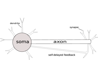
Figure 1: Sketch of an autapse: Sketch of a neuronal cell exhibiting a self delayed feedback mechanism.

We mathematically model the delayed feedback induced by an autapse (sketched in Fig. 1) by a feedback mechanism within a Hodgkin-Huxley model of the type put forward by Pyragas del . By an additional pathway in the dynamics of the membrane potential we consider the autapse leading to a delayed stimulus $I_{\mathrm{\tau}}(t)$. Particularly, we consider an excitable dynamics for the membrane potential $V(t)$, reading:

$$C\frac{\mathrm{d}V(t)}{\mathrm{d}t}= -n^{4}(t)g_{\mathrm{K}}^{\mathrm{max}}\left(V(t)-V_{\mathrm{K}}\right)-g_{\mathrm{L}}\left(V(t)-V_{\mathrm{L}}\right)-$$

$$-m^{3}(t)h(t)g_{\mathrm{Na}}^{\mathrm{max}}\left(V(t)-V_{\mathrm{Na}}\right)+I_{\mathrm{\tau}}(t)\,$$

wherein the autaptic delayed stimulus

$$I_{\mathrm{\tau}}(t)= \epsilon\left[V(t-\tau)-V(t)\right]\,,$$ (2)

is proportional to the difference of the membrane potential at time $t$ and that at an earlier time $t-\tau$. Here, $\epsilon$ corresponds to the coupling strength of the autapse mechanism and the finite delay time $\tau$ refers to the specific time delay caused by the autapse which is due to a finite signal propagation speed. The delay time $\tau$ is representing the elapsed time associated with the axonal propagation prior to the signal recurring onto the neuron; $V(t-\tau)$ is the membrane potential at the earlier time t-$\tau$.

The autaptic delayed stimulus in Eq. 2 results in an excitatory coupling mechanism in which spiking of a cell at an earlier time $t-\tau$ favors the initiation of a spiking event of the same cell at time $t$. We note, that the ansatz for the delayed self-stimulus corresponds to electrotonic interaction, i.e. we consider an idealized situation wherein the autaptic delayed stimulus is proportional to the difference of the pre- and post-synaptic membrane potentials. Moreover, as autapses are typically formed by chemical synapses, our modeling simulates the complex biophysical temporal evolution of the synaptic conductance by invoking a constant coupling strength $\epsilon$.

In Eq. (II), $C$ denotes the membrane capacitance, $V(t)$ the time-dependent membrane potential, $V_{\mathrm{L}}$ the leakage potential, $V_{\mathrm{K}}$ and $V_{\mathrm{Na}}$ the reversal potentials for the potassium and sodium currents. The leakage conductance is given by $g_{\mathrm{K}}$, the potassium and sodium maximum conductances read $g_{\mathrm{K}}^{\mathrm{max}}$ and $g_{\mathrm{Na}}^{\mathrm{max}}$, respectively. The functions $m(t)$, $n(t)$ and $h(t)$ in Eq. (II) denote the so-called stochastic gating variables (see below), describing the mean fraction of open gates of the sodium and potassium channels at time $t$. The typical values of parameters in our numerical simulation are those of the original Hodgkin-Huxley model hh ; i.e., $C$=1 $\mathrm{\mu F/cm^{2}}$, $g_{\mathrm{K}}^{\mathrm{max}}=120\mathrm{mS/cm^{2}}$, $g_{\mathrm{Na}}^{\mathrm{max}}=36\mathrm{mS/cm^{2}}$, $g_{\mathrm{L}}=0.3\mathrm{mS/cm^{2}}$, $V_{\mathrm{K}}=-77\mathrm{mV}$, $V_{\mathrm{Na}}=50\mathrm{mV}$ and $V_{\mathrm{L}}=54.4\mathrm{mV}$.

The stochastic dynamics of the gating variables $m(t)$, $n(t)$ and $h(t)$ depend on the voltage-dependent opening and closing rates $\alpha_{i}(V)$ and $\beta_{i}(V)$ ($i=m,h,n$), which read hh :

$$\alpha_{m}(V) =\frac{0.1(V+40)}{1-\exp\left\{-\,(V+40)/10\right\}}\,,$$ (3a)

$$\beta_{m}(V) =4\,\exp\left\{-\,(V+65)/18\right\}\,,$$ (3b)

$$\alpha_{h}(V) =0.07\,\exp\left\{-\,(V+65)/20\right\}\,,$$ (3c)

$$\beta_{h}(V) =\frac{1}{1+\exp\left\{-\,(V+35)/10\right\}}\,,$$ (3d)

$$\alpha_{n}(V) =\frac{0.01(V+55)}{1-\exp\left\{-\,(V+55)/10\right\}}\,,$$ (3e)

$$\beta_{n}(V) =0.125\,\exp\left\{-\,(V+65)/80\right\}\,.$$ (3f)

The resulting stochastic dynamics is then modeled by a Fokker-Plank-type dynamics for the individual gates. Specifically, this dynamics emerges within a large system size-expansion of the underlying Markovian master-equation dynamics for the dynamics of the number of open gates noi1 ; tuckwell . This so obtained Langevin-dynamics is then interpreted in the It$\hat{o}$ sense, reading explicitly:

$$\frac{\mathrm{d}i}{\mathrm{dt}}=\alpha_{i}(V)(1-i)-\beta_{i}(V)i+\xi_{i}(t),$$ (4)

with $i=m,h,n$. Here, $\xi_{i}(t)$ ($i=m,h,n$) denote independent Gaussian white noise sources with vanishing mean and auto-correlation functions:

$$\langle\xi_{m}(t)\xi_{m}(t^{\prime})\rangle =\frac{(1-m)\alpha_{m}+m\beta_{m}}{N_{Na}}\delta(t-t^{\prime}),$$ (5a)

$$\langle\xi_{h}(t)\xi_{h}(t^{\prime})\rangle =\frac{(1-h)\alpha_{h}+h\beta_{h}}{N_{Na}}\delta(t-t^{\prime}),$$ (5b)

$$\langle\xi_{n}(t)\xi_{n}(t^{\prime})\rangle =\frac{(1-n)\alpha_{n}+n\beta_{n}}{N_{K}}\delta(t-t^{\prime}).$$ (5c)

Note, that the noise strengths are determined by the number of potassium and sodium channels $N_{\mathrm{K}}$ and $N_{\mathrm{Na}}$. Throughout this work we assume constant ion channel densities; i.e. following the original Hodgkin-Huxley model we use $18$ for potassium and $60$ for the sodium channels per $\mu\mathrm{m}^{2}$ hh . An integration step $\Delta t=0.001\,\mathrm{ms}$ was used in the simulations and for the generation of the Gaussian distributed random numbers, the Box-Muller algorithm bm was used.

III Deterministic dynamics

In the absence of both, the delayed feedback, i.e. $\epsilon=0$, and zero noise strength, with the latter being formally achieved by $N_{\mathrm{Na}}\to\infty$ and $N_{\mathrm{K}}\to\infty$, the original Hodgkin-Huxley dynamics are recovered. These exhibit a single stable fixed point, which is the rest state with the rest potential $V_{\mathrm{rest}}\approx-65\,\mathrm{mV}$. Any temporary disturbance, e.g. caused by an applied external current stimulus, decays and the system relaxes back to the rest state. Note that upon a proper choice of the initial condition, a single action potential may occur, before the system relaxes to the rest state textbook .

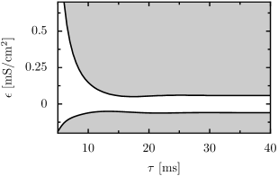
Figure 2: The phase diagram $\epsilon-\tau$ for repetitive firing within the Hodgkin Huxley model containing the delay coupling strength $\epsilon$ is depicted vs. the delay time $\tau$. The two black solid lines indicate the boundaries of critical coupling strength $\epsilon$ versus the delay time $\tau$ at which the behavior changes from the rest state to a repetitive firing. The gray areas give the parameter regime for which repetitive firing is observed.

In presence of the autaptic delay coupling, the fixed point solution remains stable, but upon increasing the delay time parameter $\tau$, there emerges now a stable, oscillatory solution, presenting repetitive (tonic) spiking. To investigate this repetitive spiking behavior in more detail, we systematically varied the two parameters ($\epsilon$ and $\tau$) of the delay coupling scheme. In doing so, we determined the first occurrence of repetitive firing after a spike was created. The resulting phase diagram with the positive and negative critical coupling strength $\epsilon_{c}^{+}(\tau)$ and $\epsilon_{c}^{-}(\tau)$, respectively, is depicted in Fig. 2. We point out the resulting asymmetry between positive and negative coupling $\epsilon$.

For sub-threshold coupling strength, i.e. $\epsilon_{c}^{-}(\tau)<\epsilon<\epsilon_{c}^{+}(\tau)$ (in the white regions of Fig. 2), excitations die out and the system relaxes to the rest state. For supra-threshold coupling, i.e. $\epsilon>\epsilon_{c}^{+}(\tau)$ or $\epsilon<\epsilon_{c}^{-}(\tau)$ a repetitive firing is observed. If the delay time becomes shorter than the refractory time interval, being ca. $12\,\mathrm{ms}$, which is the time the system needs for spiking and returning to the rest state, the modulus of the critical coupling strength of the bifurcation increases drastically. This is due to the fact, that in the so-called undershoot phase (i.e. the part of the course of the action potential when the membrane potential is smaller than the membrane potential at rest) the neuron is rather insensitive to any stimuli. Hence, a stronger coupling strength is needed in order to excite the system from the undershoot phase and to obtain repetitive firing. In case of larger delay the value of the critical coupling saturates. For longer delay times more than one spike may fit into time interval given by $\tau$. Consequently, doublets, triplets and multiplets may appear.

Below, we shall present examples where we have chosen $\tau=35$$\,\mathrm{ms}$ and used a positive coupling strength. The critical value for repetitive firing corresponds to $\epsilon_{c}^{+}=0.059\,\mathrm{mS/cm^{2}}$. For larger coupling $\epsilon>\epsilon_{c}^{+}(\tau)$ an action potential induces repetitive firing. In section IV we refer to this regime as supra-threshold delay coupling regime. In case of lower coupling strength; i.e. $\epsilon<\epsilon_{c}^{+}(\tau)$ the state of a repetitive firing is excitable and noise is needed to support the repetition of an action potential. In the next section IV this regime will be addressed as sub-threshold delay coupling regime. Remarkably, for negative coupling $\epsilon<0$ one finds an overall similar similar behavior that differs, however, quantitatively (not shown).

IV Stochastic dynamics of the Hodgkin-Huxley model with delayed feedback

Figure 3: Simulated spike-trains: (a) Membrane potential $V(t)$ from the stochastic Hodgkin-Huxley model in absence of feedback, i.e. with $\epsilon=0$ versus time $t$; (b) $V(t)$ versus time $t$ in presence of finite feedback of strength $\epsilon=0.07\mathrm{mS/cm^{2}}$ exhibiting repetitive spiking for a chosen delay time $\tau=35$$\,\mathrm{ms}$. The number of potassium ion channels is set to $N_{\mathrm{K}}=300$ and those of the sodium ion channels to $N_{\mathrm{Na}}=1000$. The spontaneous, i.e. noise induced, action potentials exhibit a bursting-like behavior in case of the delay coupling (b). In (a) we indicated with the double-arrow line a typical occurring noise-induced interspike interval $T_{i}$.

In Fig. 3 the simulated membrane potential $V(t)$ is shown for an exemplarily chosen noise level and for two cases, namely in panel (a) without delay coupling ($\epsilon=0$) and in panel (b) with a finite delay coupling $(\epsilon>0$). In absence of delay coupling the occurrence of spontaneous, i.e. noise induced actions potentials occur irregular while a characteristic bursting pattern can be detected in presence of finite delay-coupling $\epsilon$.

In order to explain the spiking dynamics quantitatively, we determined the time intervals between two spike events $T_{i}$, see in Fig. 3(a), as obtained from simulations of the stochastic Hodgkin-Huxley model with delayed feedback coupling, cf. Eq. (II). Note that in order to detect the occurrences of action potentials from the simulated membrane potential dynamics $V(t)$, we did define a specific threshold barrier for detection. In particular, whenever the membrane potential $V(t)$ exceeds the value of $0\,\mathrm{mV}$, the occurrence of an action potential is assigned. In fact, the so determined spike occurrences depend only weakly on the actual choice of the detection barrier Schmid_EPL .

These observed stochastically emerging interspike intervals $T_{i}$ the render the (normalized) interspike interval histograms (ISIH) and the mean interspike interval $\langle T\rangle$

$$\langle T\rangle=\frac{1}{N}\sum\limits_{i=1}^{N}T_{i}\,,$$ (6)

where $N$ denotes the number of spikes obtained in the individual numerical simulation. The bin width for the histograms has been set at $0.2\,\mathrm{ms}$. Both these quantities form the basis of our analysis of spike trains.

We begin this study with the dynamics of zero delay coupling for the neuron, i.e. with $\epsilon=0$. The distribution of the interspike intervals at a fixed channel noise intensity is depicted in Fig. 4. For large time intervals, the distribution decays exponentially. Small time intervals are suppressed because of the neuron’s refractory state. For $\epsilon=0$ the ISIH exhibits one broad maximum located around the internal time scale ${\cal T}_{\mathrm{int}}$ . This time scale systematically diminishes with increasing noise level Schmid_EPL ; Lindner . The minimal time scale for undistorted spikes is around the refractory time of $\approx 12\,\mathrm{ms}$.

In presence of noise and finite feedback coupling, the neuron still can return to its fix-point with nonvanishing probability. This is why the peak at the intrinsic time scale and a broad exponential decay is still detected in the ISIH in Fig. 4. However, the ISIHs become multimodal in case of finite, nonvanishing feedback. Several maxima occur at larger time intervals and, in between, a number of deep dips are observed. Such forms of the distributions of the ISIH are indicators of an enhanced coherence sy0 ; Lindner . Whereas in the sub-threshold regime (dashed line) the additional extrema merely show up, they become increasingly dominant in the case of supra-threshold coupling (note the logarithmic scale of the ordinate in Fig. 4).

IV.1 Sub-threshold delay coupling: $\epsilon<\epsilon_{c}^{+}(\tau)$

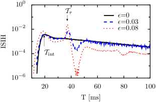
Figure 4: (Color online) Interspike interval histograms (ISIH) versus the interspike interval $T$ of the stochastic Hodgkin-Huxley model with a delay coupling mechanism at different coupling strengths $\epsilon$, as indicated in the figure in units of $\,\mathrm{mS/cm^{2}}$. The bin width for $T$ has been chosen throughout this work at $0.2\,\mathrm{ms}$. The chosen number of potassium ion channels is $N_{\mathrm{K}}=150$, while the number of sodium ion channels is set at $N_{\mathrm{Na}}=500$. The delay time $\tau$ is set at $35$$\,\mathrm{ms}$.

In the case of sub-threshold coupling the repetitive oscillatory spiking is noise supported, as a non-vanishing delayed stimulus $I_{\mathrm{\tau}}(t)$ shifts the stable fix-point towards the threshold for excitation. Consequently, the generation of spikes becomes more likely. However, the dynamics is still excitable; i.e. a threshold still exists and noise is needed to induce its excitation. Consequently, a sub-threshold delayed stimulus favors some characteristic interspike interval time ${\cal T_{\tau}}$. As far as the system remains excitable, an activation time ${\cal T}_{\mathrm{act}}$ after the delayed stimulus did set in is necessary in order to create the next noise-induced spike. Therefore, the time ${\cal T}_{\tau}$ is not equal to the delay time $\tau$, but equals the sum of the delay time and an activation time ${\cal T}_{\mathrm{act}}$, being around $2\,\mathrm{ms}$ in this considered case.

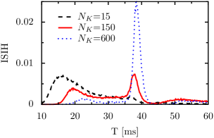
Figure 5: (Color online) Interspike interval histogram (ISIH) vs. interspike duration $T$ for different noise levels corresponding to different number of sodium and potassium channels as indicated. The chosen delay time is : $\tau=35\,\mathrm{ms}$; the coupling strength is set at $\epsilon=0.03\,\mathrm{mS/cm}^{2}<\epsilon_{c}^{+}(\tau)$ and $N_{\mathrm{Na}}=\frac{10}{3}N_{\mathrm{K}}$.

In addition, there occurs a suppression of certain time scales when the delay coupling is applied to the neuronal dynamics, cf. Fig. 4. For positive $\epsilon$ the system favors frequencies associated to the time ${\cal T}_{\tau}$ and suppresses frequencies slightly larger than those. The feedback hinders the generation of spikes by noise if the feedback current $I_{\mathrm{\tau}}(t)$ approaches values around the polarized refractory period.

In the sub-threshold regime the intrinsic time scale ${\cal T}_{\mathrm{int}}$ and correspondingly the height and the position of the associated peak distinctly depends on the noise level. In Fig. 5 we depict results from simulations for different noise levels, i.e. different numbers of embedded ion channels. With increasing noise level the generation of spontaneous spikes by noise gains influence substantially. As a result, the intrinsic time scale becomes changed and the larger time intervals reflect the broad, exponentially decaying ISIH. The former sharply peaked maximum at ${\cal T}_{\tau}$ switches towards a noise supported broader peak at smaller times, and the maximum shifts with growing noise towards the minimal time for a interspike interval located at the refractory time. Interspike intervals around this minimal time are promoted mainly by the presence of noise. They do not necessarily relate to the delay mechanism. In contrast, the time scale ${\cal T}_{\tau}$ induced by the delayed feedback is only slightly affected by the noise level. This is a somewhat striking feature recalling the fact that in the case of an excitable dynamics these spikes in fact require the presence of noise to become activated. The robustness of the positions of the time scales as well as their separation from the noisy time scale in terms of the resulting bimodal shape of the ISIH thus indicates a noisy synchronization phenomenon sy1 ; sy2 ; sch ; ku .

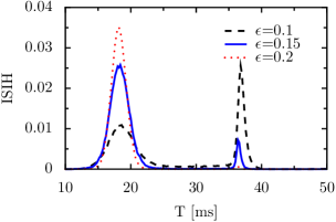
Figure 6: (Color online) Interspike interval histogram (ISIH) for different values of the supra-threshold coupling strength $\epsilon>\epsilon_{c}^{+}(\tau)$: The distribution of the interspike intervals is depicted for fixed delay time $\tau=35\,\mathrm{ms}$, the numbers of ion channels are $N_{\mathrm{K}}=150$ and $N_{\mathrm{Na}}=500$. The values of the coupling strengths indicated in the plot are in units of $\,\mathrm{mS/cm^{2}}$.

IV.2 Supra-threshold delay coupling: $\epsilon>\epsilon_{c}^{+}(\tau)$

We next consider the case with coupling strengths beyond the critical strength, i.e., $\epsilon>\epsilon_{c}^{+}(\tau)$. Here, the spikes repeat deterministically. However, noise-induced skipping of spikes sch-a ; LNP leads to a transition from the oscillatory state with repetitive firing to the excitable state. In turn, the back-transitions from the excitable to the oscillatory state are caused by noise-induced spontaneous spikes, cf. Fig. 3. The spikes repeated deterministically lead to sharp peaks in the ISIH, while the noise-induced back-transitions from excitable to the oscillatory state result in a broad distribution with exponentially decaying tail. In Fig. 6, the resulting ISIH is depicted for various supra-threshold coupling strengths. Upon the chosen parameter values for the noise level, i.e. the number of sodium and potassium ion channels, and the coupling parameters $\epsilon$ and $\tau$, the ISIH therefore exhibits sharp peaks and more or less pronounced broad background: For stronger coupling or weaker noise the broad background diminishes. Contrarily, the peak height at ${\cal T}_{\tau}$ shows a strong dependence on the noise level, indicating the competitive interplay between channel noise and the delayed feedback mechanism: With increasing noise level the height of the peak at ${\cal T_{\tau}}$ decreases, while the intrinsic time scale acquires increasing influence (depicted for the sub-threshold coupling regime in Fig. 5 ). Note that we have selected the delay time ($\tau=35\,\mathrm{ms}$) so that the separation between the broad background which is peaked at the intrinsic time scale $\cal T_{\mathrm{int}}$ and the delayed induced sharp peaks at ${\cal T}_{\tau}$ and multiples thereof is educible and visible with the ISIHs, cf. Fig. 5 and Fig. 6.

Strikingly, with increasing coupling strength the multimodal structure collapses to a unimodal one, cf Fig. 6. The most probable interspike interval now centers at one value. Due to this supra-threshold driving, each spontaneous spiking event is repeated periodically and even the noise dominated scale now collapses towards a narrow peak. Note also that the distribution gains in sharpness as the coupling strength increases, cf. Fig. 6.

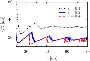
Figure 7: (Color online) Average interspike interval $\langle T\rangle$ as function of the delay time $\tau$: The mean interspike interval $\langle T\rangle$, cf. Eq. (6), is plotted versus the delay time $\tau$ for the following parameters: the used ion channel numbers are $N_{\mathrm{K}}=150$, $N_{\mathrm{Na}}=500$ and the coupling strengths are set at $\epsilon=0.1\mathrm{mS/cm^{2}}$ (black dashed line), $\epsilon=0.2\mathrm{mS/cm^{2}}$ (red dotted line), and $\epsilon=0.4\mathrm{mS/cm^{2}}$ (blue solid line).

Figure 8: The inverse of the number of spikes that fit into the delay-time interval $\kappa$ is plotted as function of the delay time $\tau$ for $N_{\mathrm{K}}=150$, $N_{\mathrm{K}}=500$ and a delay coupling strength of $\epsilon=0.4\mathrm{mS/cm^{2}}$.

Let us focus on the dependence of the interspike intervals on the delay time $\tau$. For this purpose we consider the mean interspike interval, cf. Eq. (6). This quantity inherits the characteristic dependence on $\tau$ since the ISIH shape is unimodal. Larger deviations from the mean interspike interval are found during transitions between different synchronized states where the histogram becomes multimodal.

In Fig. 7 the mean interspike interval $\langle T\rangle$ is depicted for a fixed channel noise strength. If the delay coupling mechanism does not dominate the spiking, i.e. for small supra-threshold coupling strengths, the mean interspike interval exhibits a smooth dependence on the delay time. However for larger supra-threshold driving strengths, for which the ISIH exhibits a unimodal structure consisting of a sharp peak, the mean interspike time varies with the delay time $\tau$ in an almost piecewise linear fashion, displaying sharp, triangle-like textures , cf. Fig. 7. At these sharp peak locations, the number of spikes that fit according to the intrinsic time into a full time length given by the delay time, just increases by unity with increasing delay time $\tau$. The mean interspike interval is henceforth proportional to the ratio of the delay time and the number of spikes $n$ fitting into this very delay-time interval; yielding

$$\langle T\rangle\propto\tau\big{/}n\doteq\tau\kappa\,.$$ (7)

In Fig. 8 the behavior of $\kappa$ vs. the delay time $\tau$ is depicted. At multiples of the noise-dependent intrinsic time scale, such characteristic steps do occur indeed.

We find that stronger noise intensity mimics a decrease of the coupling strength. Nearby those typical steps noise is able to induce newly generated spikes at the end of the intervals reducing thereby the ratio $\kappa$. Alternatively, the role of noise decreases the number of spikes towards the left boundary of a new synchronized region. Therefore the corresponding results at increased noise strength attain a form that is similar to the case of lower delay coupling strength.

A comparable scenario has been reported in other systems such as for a noisy Van der Pol dynamics, see in Refs. AMJP ; prl04 ; sch2 near the Hopf bifurcation, for semiconductor superlattices sh and stochastic excitable dynamics sch . We find that noise can induce oscillations with a well-defined time scale, and the simultaneous application of a delay of duration $\tau$ is able to stabilize this orbit.

IV.3 Phase oscillator modeling

We have seen that the neuron behaves almost like an oscillatory system whenever the delay coupling rules the dynamics. This brings to mind a description in terms of a phase oscillator model which we develop next. Let us assign an intrinsic frequency by $\omega=2\pi/{\cal T}_{\mathrm{int}}$. As pointed out above, the autaptic feedback leads to a stabilization of the internal rhythmicity as determined by the model parameters. This in turn results in synchronized patterns, cf. Fig. 8.

Therefore we investigate the question whether the observed synchronization in this studied neuronal model with autapse can be characterized by a Kuramoto-type model acebron of a phase oscillator including delayed feedback? Put differently, upon neglecting the details of the shape of the spike trains the essential information can be reduced to the phase of the oscillatory neuron.

Let us next compare our findings with the results obtained from a pure phase dynamics. Accordingly, the proposed dynamics for the underlying phase is modeled as:

$$\dot{\phi}=\omega-A\sin\left[\phi(t)-\phi(t-\tau)\right]\,,$$ (8)

where $\omega$ denotes the angular intrinsic frequency of the oscillator and $A$ is the delay-coupling strength. Searching for solutions with fixed frequency $\Omega$, we make the Ansatz:

$$\phi(t)=\Omega\,t\,.$$ (9)

The resulting, self-consistent equation reads schuster1 ; schuster2 ; morelli :

$$\Omega=\omega-A\sin\left[\Omega\tau\right]\,,$$ (10)

which was solved numerically. Comparing this phase oscillator dynamics with our oscillatory stochastic neuron dynamics exhibiting an autapse, we make the following parameter identification, i.e., $\Omega=2\pi/\langle T\rangle$ and obtain from an expansion in small delay time $\tau$ the relation $A=1/{\cal T}_{\mathrm{int}}$. In Fig. 9 we present the comparison between the Hodgin-Huxley modeling and the the phase oscillator modeling: Even though the quantitative behavior is different, a good qualitative agreement is detected. The positions of the spikes where the autapse model jumps between bursts of different number of multiplets are nicely reproduced by this simplified phase oscillator modeling. A further improvement of the modeling would require a more optimal determination of the $\tau$-dependent parameters of this Kuramoto model with feedback.

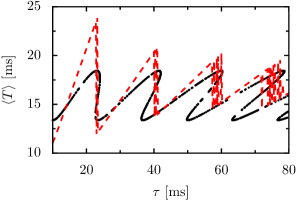
Figure 9: (Color online) Comparison of the stochastic, neuronal dynamics Hodgkin-Huxley model including feedback, Eqs. (II, 3, 4, 5) with the dynamics of the feedback assisted Kuramoto-type phase oscillator model, Eq. (8). The mean interspike interval (red dashed lines) is the result of the numerical integration of the stochastic Hodgkin-Huxley model with delayed feedback; there is quantitative good agreement between period of oscillations as obtained from a phase oscillator dynamics of the Kuramoto-type delayed feedback model (solid black line). Regions with multiple solutions in the phase model correspond to discontinuous jumps between different types of multiplets in the Hodgkin-Huxley model. The parameters for the neuronal modeling are chosen as $N_{\mathrm{K}}=150$, $N_{\mathrm{Na}}=500$ and $\epsilon=0.4\,\mathrm{mS/cm^{2}}$; those of the phase oscillator are given by oscillator frequency $\omega=2\pi/15.5\,\mathrm{ms}$ and feedback strength $A=1/15.5\,\mathrm{ms}$.

V Conclusion

With this work we have investigated the effect of delayed feedback on the dynamics of a stochastic Hodgkin-Huxley neuron. Using the original Hodgkin-Huxley parameters, we simulated numerically the stochastic Hodgkin-Huxley model taking into account the effects of intrinsic channel noise. A Pyragas-like delayed feedback mechanism is employed to model the autapse phenomena, in which a neuron’s dendrite back-couples to itself. The two basic parameters used in our study are the strength of the autapse-coupling $\epsilon$ and the time-delay $\tau$ resulting from the finite length of the self-connecting dendrite.

We have found that the neuron dynamics exhibits intriguing new times scale that stem from the autaptic connection. Since the rest state of the neuron is always stable, noise or an initial spike is necessary to create activity, i.e. the spiking dynamics. For a small number of $\mathrm{Na}$ and $\mathrm{K}$ channels, the noise becomes sizable and the excitory dynamics remains practically unaffected by the delay. In contrast, smaller noise levels and stronger coupling strengths induce a different synchronization phenomena between the delay time and the intrinsic (also noise dependent) time scales. The delay time and these intrinsic time scales determine how many spikes will be created and become subsequently locked during one delay epoch. We further underline that our exemplary study can be mimicked qualitatively in terms of a reduced description given by a Kuramoto phase dynamics with built-in feedback.

We have shown, that the delayed feedback mechanism serves as a control option for adjusting the peaked distribution of interspike intervals, being of importance for memory storage sto and stimulus-locked short-term dynamics in neuronal systems a1 . One may therefore speculate whether nature adopted the autapse phenomena for frequencies-filtering in presence of unavoidable intrinsic channel noise.

VI Acknowledgments

This work has been supported by the China Scholarship Council (CSC), the Volkswagen Foundation (projects I/80424 and I/80425) and the Bernstein Center for “Computational Neuroscience” Berlin.

References

- (1) G. M. Süel, J. García-Ojalvo, L. M. Liberman and M. B. Elowitz, Nature 440, 545 (2006).
- (2) J. L. Cabrera and J. G. Milton, Phys. Rev. Lett. 89, 158702 (2002).
- (3) J. Hizanidis and E. Schöll, Phys. Rev. E 78, 066205 (2008).
- (4) T. Erneux and J. Grasman, Phys. Rev. E 78, 026209 (2008).
- (5) W. Bao, Z. Li, L. Zhou and Z. Gao, Phys. Rev. E 79, 016214 (2009).
- (6) S. Rüdiger and L. Schimansky-Geier, J. Theor. Biol. 259, 96 (2009).
- (7) C. Masoller, M. C. Torrent and J. García-Ojalvo, Phys. Rev. E 78, 041907 (2008).
- (8) C. Beta, M. Bertram, A. S. Mikhailov, H. H. Rotermund and G. Ertl, Phys. Rev. E 67, 046224 (2003).
- (9) T. Prager, H. Lerch, L. Schimansky-Geier and E. Schöll, J. Phys. A: Math. Theor. 40, 11045 (2007).
- (10) G. C. Sethia, J. Kurths and A. Sen, Phys. Lett. A 364, 227 (2007).
- (11) M. A. Arteaga, M. Valencia, M. Sciamanna, H. Thienpont, M. López-Amo and K. Panajotov, Phys. Rev. Lett. 99, 023903 (2007).
- (12) A. B. Karabelas and D. P. Purpura, Brain Res. 200, 467 (1980).
- (13) G. Tamás, E. H. Buhl and P. Somogyi, J. Neurosci.17, 6352 (1997).
- (14) J. M. Bekkers, Curr. Biol. 8, R52 (1998).
- (15) K. Ikeda and J. M. Bekkers, Curr. Biol. 16, R308 (2006).
- (16) H. Van Der Loos and E. M. Glaser, Brain Res. 48, 355 (1972).
- (17) J. Lübke, H. Markram, M. Frotscher and B. Sakmann, J. Neurosci. 16, 3209 (1996).
- (18) B. Lindner, J. García-Ojalvo, A. Neiman and L. Schimansky-Geier, Phys. Rep. 392, 321 (2004).
- (19) L. Gammaitoni, P. Hänggi, P. Jung and F. Marchesoni, Rev. Mod. Phys. 70, 223 (1998).
- (20) P. Hänggi, ChemPhysChem 3, 285 (2002).
- (21) G. Schmid, I. Goychuk and P. Hänggi, Europhys. Lett. 56, 22 (2001).
- (22) P. Jung and J. W. Shuai, Europhys. Lett. 56, 29 (2001).
- (23) L. Meinhold and L. Schimansky-Geier, Phys. Rev E 66, 050901R (2002).
- (24) G. Schmid, I. Goychuk and P. Hänggi, Phys. Biol. 1, 61 (2004).
- (25) G. Schmid, I. Goychuk and P. Hänggi, Phys. Biol. 3, 248 (2006).
- (26) G. C. Sethia and A. Sen, Phys. Lett. A 359, 285 (2006).
- (27) A. Pikovsky, M. Rosenblum and J. Kurths, Synchronization: A Universal Concept in Nonlinear Sciences (Cambridge University Press, Cambridge, 2003).
- (28) A. M. Lacasta, F. Sagués and J. M. Sancho, Phys. Rev. E 66, 045105(R) (2002).
- (29) L. Callenbach, P. Hänggi, S. J. Linz, J. A. Freund and L. Schimansky-Geier, Phys. Rev. E 65, 051110 (2002).
- (30) J. A. Freund, L. Schimansky-Geier and P. Hänggi, Chaos 13, 225 (2003).
- (31) R. F. Fox and Y. Lu, Phys. Rev. E 49, 3421 (1994).
- (32) A. Ochab-Marcinek, G. Schmid, I. Goychuk and P. Hänggi, Phys. Rev. E 79, 011904 (2009).
- (33) A. L. Hodgkin and A. F. Huxley, J. Physiol. 117, 500 (1952).
- (34) J. A. White, J. T. Rubinstein and A. R. Kay, Trends Neurosci., 23, 131 (2000).
- (35) K. Pyragas, Phys. Lett. A 170, 421 (1992).
- (36) H. C. Tuckwell, J. Theoret. Biology 127, 427 (1987).
- (37) G. E. P. Box and M. E. Muller, Ann. Math. Stat. 29, 610 (1958).
- (38) J. Keener and J. Sneyd, Mathematical Physiology (Springer-Verlag, New York, 1998)
- (39) G. Schmid, I. Goychuk, and P. Hänggi, Physica A 325, 165 (2003).
- (40) G. Schmid, I. Goychuk, and P. Hänggi, Lecture Notes in Physics, 625, 195 (2003).
- (41) C. Zhou and J. Kurths, Chaos 13, 401 (2003).
- (42) P. Hänggi and P. Riseborough, Am. J. Phys. 51, 347 (1983).
- (43) N. B. Janson, A. G. Balanov and E. Schöll, Phys. Rev. Lett. 93, 010601 (2004).
- (44) A. Pototsky and N. Janson, Phys. Rev. E 76, 056208 (2007).
- (45) J. A. Acebrón, L. L. Bonilla, C. J. P. Vicente, F. Ritort and R. Spigler, Rev. Mod. Phys. 77, 137 (2005).
- (46) H. G. Schuster and P. Wagner, Prog. Theor. Phys. 81, 939 (1989).
- (47) E. Niebur, H. G. Schuster and D. M. Kammen, Phys. Rev. Lett. 67, 2753 (1991).
- (48) L. G. Morelli, S. Ares, L. Herrgen, C. Schröter, F. Jülicher and A. C. Oates, HFSP Journal 3, 55 (2009).
- (49) H. S. Seung, J. Comput. Neurophysiol. 9, 171 (2000).
- (50) P. A. Tass, Europhys. Lett. 59, 199 (2002).