Abundances and rotational temperatures of $C_{2}$ interstellar molecule toward six reddened early type stars

Abstract

Using high resolution ($\sim$85,000) and high signal-to-noise ratio ($\sim$200) optical spectra acquired with ESO/UVES spectrograph, we determined interstellar column densities of $C_{2}$ for six Galactic lines of sight with E(B-V)’s ranging from 0.33 to 1.03. For the purpose we identified and measured absorption lines belonging to the (1,0), (2,0) and (3,0) Phillips bands $\rm A^{1}\Pi_{u}-X^{1}\Sigma^{+}_{g}$. Identification of a few lines of the $C_{2}$ (4,0) Phillips system towards HD 147889 is reported. The curve of growth method is applied to equivalent widths for the determination of column densities of individual rotational levels of $C_{2}$. Excitation temperature is extracted from the rotational diagrams. Physical parameters of the intervening molecular clouds: gas kinetic temperatures and densities of collision partners were estimated from comparison with the theoretical model of excitation of $C_{2}$ (van Dishoeck & Black, 1982).

1 Introduction

Diatomic carbon is found in a variety of celestial bodies such as comets ($C_{2}$ Swan band - Mayer & O’dell (1968); Lambert & Danks (1983); Ballik-Ramsay and Phillips bands - Johnson et al. (1983); Gredel et al. (1989)), the Sun (Swan band - Grevesse & Sauval (1973); Lambert (1978)), in carbon stellar atmospheres (Swan, Ballik-Ramsay and Phillips bands - Querci et al. (1971)), circumstellar shells of carbon rich post-AGB stars (Phillips and Swan bands - Bakker et al. (1996); Bakker et al. (1997)) and in interstellar clouds.

In the interstellar medium, $C_{2}$ was first detected by Souza & Lutz (1977). They observed absorption lines of the (1,0) Phillips band $\rm A^{1}\Pi_{u}-X^{1}\Sigma^{+}_{g}$. Lines of the (2,0) Phillips system were first tentatively detected in interstellar clouds by Chaffee & Lutz (1978). The evident demonstration of the band was shown by Chaffee et al. (1980). The Phillips band (3,0) was discovered only by van Dishoeck & Black (1986). Some $C_{2}$ lines of the (4,0) Phillips band in direction to HD 204827 were shown by Hobbs et al. (2008) (few of very weak and difficult to measure lines of this band are demonstrated here for the first time toward HD 147889).

$C_{2}$ is particularly interesting because it is the simplest multi-carbon molecule. Its abundances give information on the chemistry of interstellar clouds, especially on the pathway to the formation of long chain carbon molecules which may be connected with carriers of diffuse interstellar bands (DIBs) (Douglas, 1977; Thorburn et al., 2003). Additionally, the analysis of $C_{2}$ lines allows to determine physical conditions in interstellar clouds.

In the interstellar medium, because of the very rare collisions and low temperatures, we expect only absorption lines from the ground electronic state. For $C_{2}$, there are Mulliken (discovered by Snow (1978), $D^{1}\Sigma^{+}_{u}-X^{1}\Sigma^{+}_{g}$, $\sim$2313 Å, see also - Lambert et al. (1995); Sonnentrucker et al. (2007)), F-X (first detected by Lien (1984), $\rm F^{1}\Pi_{u}-X^{1}\Sigma^{+}_{g}$, $\sim$1342 Å) and Phillips systems ($A^{1}\Pi_{u}-X^{1}\Sigma^{+}_{g}$, $\sim$ 6900-12000 Å).

$C_{2}$, as a homonuclear diatomic molecule, has a negligible dipole moment and hence radiative cooling of the excited rotational levels may go only through the slow quadrupole transitions (van Dishoeck & Black, 1982). The rotational levels are pumped by the galactic interstellar radiation field and excited effectively above the gas kinetic temperature. The rotational ladder of the electronic absorptions from the high rotational levels (here up to J”=26) are usually observed. Because of that, lines of the diatomic carbon from a long-lived ground state rotational levels are measurable and can be the sensitive diagnostic probes of conditions in molecular clouds that produce the interstellar absorption lines, in contrast to polar molecules, such as $CH$ or $CN$, where usually only a few absorption lines from the lowest rotational levels are observed.

Relative abundances of $C_{2}$ were predicted for the interstellar clouds on the basis of detailed chemical models (Black & Dalgarno, 1977; Black et al., 1978). The excitation mechanisms of $C_{2}$ have been already analysed in detail (Chaffee et al., 1980; van Dishoeck & Black, 1982).

The main purpose of this paper is to determine basic physical parameters like temperatures and densities of the intervening clouds. Four out of the six analysed objects (Table 1) were studied before, but high quality spectra from the ESO archive (Bagnulo et al., 2003) allowed to accurately measure these weak features. Broad spectral range of the UVES spectra allows us to analyse up to four bands by contrast with previous analyses usually based on single (2,0) band of the Phillips system. Simultaneous observations of different bands give possibility to compare individually determined results for each band and make results more reliable. In this paper two new objects with the interstellar absorption lines of $C_{2}$ are presented, increasing the presently available sample of interstellar clouds (24 lines of sight - see Sonnentrucker et al. (2007) - Table 13) where a detailed analysis of excitation of $C_{2}$ was made (estimates of densities and excitation temperatures).

The next section describes our data, the observations, reduction and criteria for choosing stars. In Sect. 3 we introduce methods of analysis of the observational data. General discussion and summary of our conclusions are given in Sect. 4 and 5. Discussion of individual results for each star of the sample and comparison between our results and those of previous papers is demonstrated in the Appendix.

2 The observational data

We used the archived spectroscopic observations collected using the spectrograph UVES (Dekker et al., 2000). UV-Visual Echelle Spectrograph (UVES) is the high-resolution spectrograph of the VLT fed by the Kueyen telescope of the ESO Paranal Observatory, Chile. UVES is a cross-dispersed echelle spectrograph designed to operate with high efficiency from the atmospheric cut-off at 3000 Å to the long wavelength limit of the CCD detectors (about 11,000 Å) so it is really suitable instrument allowing to observe four bands of the Phillips system in single exposure. The high-quality of UVES allows to get excellent spectra with the maximal resolution of about 85,000 (accurate value in Table 1) and signal-to-noise ratio above 200.

Table 1: Basic data for program stars (Thorburn et al. 2003, Hunter et al. 2006).

object	name	Sp/L	V	E(B-V)	R
HD 76341		O9Ib	7.17	0.49	79,000
HD 147889		B2V	7.90	1.07	98,000
HD 148184	$\chi$ Oph	B2V	4.28	0.52	81,000
HD 163800		O4V	7.01	0.60	82,000
HD 169454	V430 Sct	B1Ia	6.65	0.93	110,000
HD 179406	20 Aql	B3V	5.34	0.33	63,000

We have chosen spectra with interstellar molecular lines of $C_{2}$ towards six early-type stars (Table 1) from the UVES archive. Objects with intermediate colour excess and with one really dominant velocity component, at the resolution of observational material, were selected to make it likely that $C_{2}$ molecular lines originate from single clouds. In addition KI 7699 Å line profiles were checked for possible existence of more than one dominating Doppler components. Generally we cannot exclude existence of multiple closely-spaced components. For example, Welty & Hobbs (2001) show a very weak Doppler component in KI and CH toward HD 148184 which are not visible in our spectra. Presence of weak components should not contaminate rather weak $C_{2}$ lines. These authors also show that almost all of the program objects have multiple components in NaI; however this component may be not related to molecular ones (Bondar et al., 2007). In ultra-high resolution spectra of HD 169454, Crawford (1997) and Crawford & Barlow (1996) see two Doppler components in $C_{2}$ lines. These are yet unresolved at the UVES resolution.

The spectral analysis was made with the Dech20T code (Galazutdinov, 1992).

Spectral regions with interstellar $C_{2}$ absorption lines, especially the (3,0) and (4,0) bands, are contaminated by atmospheric lines. Our spectra were divided by spectrum of proper standard (Spica) to remove telluric lines. In this way a majority of telluric features was removed. Remaining lines were cut out one by one manually. The continuum was traced to remove broad stellar absorption features. Also possible broad DIB at 7721.7 Å (Herbig & Leka, 1991) blended with $C_{2}$ (3,0) Q(2) line was removed in this procedure.

Figure 1: The regions of the $C_{2}$ (1,0), (2,0), (3,0) and (4,0) Phillips band in the spectrum of HD 147889. Spectrum was normalised to a continuum level of 1. $C_{2}$ absorption lines are indicated. The wavelength scale has been shifted to the rest wavelength velocity frame using the interstellar KI line (7698.965 Å).

The final spectra were normalised to unity to enable measurements of the equivalent widths. The equivalent widths were measured by fitting Gaussian profile to each absorption line. At the resolution of the spectra ($\sim 3-5\,\mathrm{km}\,\mathrm{s}^{-1}$) the profiles of single molecular lines would have the shape of the instrumental profile. Expected Doppler broadening of the profiles caused by thermal and turbulent motions ($<0.7\,\mathrm{km}\,\mathrm{s}^{-1}$ - see Crawford (1997) (Table 4.)) are significantly lower.

The uncertainties of the equivalent widths ($\Delta EW$) were estimated with the IRAF splot task taking into consideration signal-to-noise ratio in the portion of spectrum close to measured $C_{2}$ line. In these cases, where continuum tracing was uncertain, additional uncertainty was estimated by changing level of continuum. The errors were propagated to the uncertainties of the determined parameters (e.g. excitation temperatures, column densities) and used in search of the best fit model parameters.

In summary, we measured absorption lines (P, Q, R branches) in bands (1,0) 10133 - 10262 Å, (2,0) 8750 - 8849 Å, (3,0) 7714 - 7793 Å. In one case, HD 147889, we were able to identify and measure interstellar absorption lines of the (4,0) 6909 - 6974 Å band (Fig. 1).

The final spectra of HD 147889, with the continuum level normalised to unity, are shown in Figure 1. Broad stellar lines were removed in the procedure of continuum tracing. There are plenty of weak absorption lines (Fig. 1) thanks to the high quality of the UVES data. Even the P(4) and Q(8) lines, which usually are blended in the (2,0) band, are well separated in all objects. A lot of $C_{2}$ lines were also found in the (3,0) band. The oscillator strengths for (4,0) are about five times weaker than those in the (2,0) and, in addition, molecular lines around 6915 Å  are seriously contaminated by telluric lines. $C_{2}$ lines of the Phillips system, seen in all spectra of the program stars, allow to identify rotational components of P, Q and R branches to high rotational levels, up to J”=16. In the spectrum of HD 147889 we managed to identify Q components up to J”=26.

3 Results and interpretation

We have identified lines of the (1,0), (2,0), (3,0) and in one case (4,0) bands of the $C_{2}$ Phillips system ($\rm A^{1}\Pi_{u}-X^{1}\Sigma^{+}_{g}$). The equivalent widths with errors of all measured interstellar lines of $C_{2}$ towards six program stars are given in Tables 2-5. Poor quality measurements of equivalent widths are marked with sign u behind the value. These uncertain values were not used in the further analysis of the column densities.

Column density of a rotational level J” may be derived from the equivalent width $W_{\lambda}$[mÅ] of the single absorption line using the relationship (Frisch, 1972)

$$N_{col}=1.13\times 10^{17}{\frac{W_{\lambda}}{f_{ij}\lambda^{2}}}~{},$$ (1)

where $\lambda$ is the wavelength in [Å], $f_{ij}$ is the absorption oscillator strength.

The energies of the lower rotational level were determined using molecular constants of Marenin & Johnson (1970). The wavelengths are generally determined from laboratory wavenumbers of Chauville et al. (1977) and Ballik & Ramsay (1963) converted to air wavelengths using Edlen’s formula following Morton (1991). Wavelengths of three lines R(2), P(2) and P(4) of the (2,0) band, absent in (Chauville et al., 1977), were computed with Douay et al. (1988) spectroscopic constants. According to Douay et al. (1988) the line positions calculated with their constants should be more accurate than the previous measurements. The oscillator strengths correspond to vibrational oscillator strengths $f_{10}=2.38\times 10^{-3}$, $f_{20}=1.44\times 10^{-3}$, $f_{30}=6.67\times 10^{-4}$, $f_{40}=2.71\times 10^{-4}$. The oscillator strengths for individual transitions were computed according to description in Bakker et al. (1996) using their code MOLLEY. Vibrational oscillator strengths were taken from Langhoff et al. (1990) for (1,0) and (2,0), Bakker et al. (1997) (citing Langhoff) (3,0) and from van Dishoeck (1983) for (4,0). Source of band origins were Chauville et al. (1977) and Ballik & Ramsay (1963).

Equation (1) is accurate for the optically thin case (when the absorption lines are on the linear part of the curve of growth). Only a few lines from the (1,0) band of HD 147889, where the equivalent widths are the largest, are evidently optically thick. Then curve of growth method was applied for the derivation of column densities instead of the equation (1). For an optically thick line we determined the turbulent velocity through the minimalization of the dispersion of column densities for each level. We checked various values of the velocity dispersion parameter ($b=\,0;\,0.5;\,1;\,1.5\,\mathrm{km}\,\mathrm{s}^{-1}$) and 0.5 $\mathrm{km}\,\mathrm{s}^{-1}$ was found to give the lowest dispersion. This value was then applied to all of the program stars. It is consistent with the value derived in other studies of molecular absorptions (e.g. Gredel et al. (1991); Crawford (1997)). The application of equation (1) to optically thick lines underestimates column densities by 28 per cent in the worst case of Q(2) (1,0) absorption line in HD 147889.

The resulting column densities for each rotational level $N_{col}(J^{\prime\prime})$, derived uncertainties and the number of measurements used to determine that value are presented in Table 6. The total $C_{2}$ column density, defined as the sum of the mean column densities of the observed levels and of the contribution of the unobserved levels estimated from the theoretical model characterised by the best-fit parameters (see below), are shown in column 5 of Table 7. There were available three Phillips bands so the column density could be maximally estimated from 9 measurements. Not every part of spectrum allows to measure very weak interstellar features of $C_{2}$. In some cases column density was derived from only one transition (e.g. for the highest rotational levels J”=10, 12, 14, 16). Absorption lines from lower levels (J”= 2 and 4) are the most populated and the easiest to be measured accurately.

Following van Dishoeck & Black (1982) we present derived column densities in form of rotational diagrams (Fig. 2) where weighted relative column densities $-ln[5N_{col}(J^{\prime\prime})/(2J^{\prime\prime}+1)N_{col}(2)]$ are plotted versus energy of lower level E”/k (where E” is the energy of the rotational level J” and k is the Boltzmann constant). The errorbars correspond to the derived uncertainties. The slope of a straight line on this diagram is nicely connected to the excitation temperature, $a=-1/T_{exc}$. It is well known from previous works (e.g. van Dishoeck & Black (1982)) that populations of all rotational levels cannot be characterised by a single rotational temperature. The lowest J” levels are described by the lower excitation temperature than higher levels. Such behaviour of the rotational levels was nicely described in the model of excitation of $C_{2}$ by van Dishoeck & Black (1982). In this model, the molecule is heated by the electronic transitions from the ground state, and subsequently cooled down through cascading to the ground electronic state through excited vibrational levels. Because $C_{2}$ is a homonuclear species, the mechanism of cooling is inefficient and the high rotational levels are significantly populated. The population of the lowest rotational levels is influenced by the collisions with the gas, mainly atomic and molecular hydrogen (hence the density of collision partners $n_{c}=n_{H}+n_{H_{2}}$).

Table 2: Observation summary table with equivalent widths [mÅ] of $C_{2}$ (1,0) Phillips lines toward program stars. In table are also $B(N^{\prime\prime}=J^{\prime\prime})$ - branch identification ($J^{\prime\prime}$ - low rotational level) and $\lambda$ - wavelength in air in Å (see text for the references).

$B(N^{\prime\prime}=J^{\prime\prime})$	HD76341	HD147889	HD148184	HD163800	HD169454	HD179406	$\lambda$ [Å]
$R(6)$		$8.3\pm 1.5$	$1.6\pm 1.0$	$0.6\pm 0.5u$	$4.0\pm 1.0$	$3.2\pm 1.0$	10133.603
$R(8)$		$5.8\pm 1.5$	$2.4\pm 1.5$	$1.0\pm 0.7$	$0.7\pm 1.3$	$1.9\pm 0.8u$	10133.854
$R(4)$	$2.2\pm 1.1$	$15.6\pm 1.4$	$6.5\pm 1.6$	$3.6\pm 1.3$	$7.0\pm 1.2$	$8.7\pm 1.1$	10135.149
$R(10)$		$3.4\pm 2.2$		$0.5\pm 0.5u$		$2.0\pm 1.4u$	10135.923
$R(2)$	$3.2\pm 1.2$	$17.1\pm 1.4$		$2.6\pm 1.0$	$12.5\pm 1.1$	$6.1\pm 1.5$	10138.540
$R(12)$			$0.5\pm 0.9$				10139.805
$R(0)$	$1.6\pm 1.0$	$12.4\pm 1.4$	$4.0\pm 1.2$	$3.8\pm 1.0$	$14.3\pm 1.0$	$5.2\pm 1.0$	10143.723
$R(14)$				$0.8\pm 0.5$			10145.505
$Q(2)$		$22.1\pm 1.4$	$6.4\pm 0.5$	$4.3\pm 1.3u$	$21.0\pm 1.4$	$9.0\pm 1.3$	10148.351
$Q(4)$	$2.6\pm 1.2$	$20.3\pm 1.6$	$7.2\pm 1.2$	$3.2\pm 1.4u$	$12.5\pm 1.0$	$11.4\pm 1.2$	10151.523
$P(2)$		$5.6\pm 1.4$		$2.0\pm 0.9$	$3.9\pm 1.2$		10154.897
$Q(6)$		$17.1\pm 1.4$	$4.4\pm 1.3$	$6.0\pm 1.4u$	$5.9\pm 1.0$	$6.3\pm 1.0$	10156.515
$Q(8)$	$0.7\pm 0.7$	$13.7\pm 1.2$	$2.8\pm 1.5$	$4.6\pm 1.3$	$4.5\pm 1.2$	$4.2\pm 1.2$	10163.323
$P(4)$	$0.3\pm 0.3u$	$8.8\pm 1.5$	$2.1\pm 0.9$		$2.8\pm 1.0$		10164.763
$Q(10)$	$0.8\pm 0.8$	$10.6\pm 1.6$	$2.6\pm 1.2$		$1.7\pm 0.8$	$3.0\pm 1.0$	10171.963
$P(6)$		$8.8\pm 1.5$	$1.2\pm 0.9$		$3.0\pm 0.9$		10176.252
$Q(12)$		$4.7\pm 1.2$			$0.9\pm 0.9u$		10182.434
$P(8)$		$4.9\pm 1.3$	$1.4\pm 0.7$		$1.3\pm 0.6$		10189.693
$Q(14)$		$3.3\pm 1.2$					10194.755
$P(10)$		$2.8\pm 1.6$					10204.998
$Q(16)$		$4.0\pm 1.6$					10208.931
$P(12)$		$1.8\pm 0.9$					10222.171
$P(14)$		$1.7\pm 0.8$					10241.246
$Q(18)$		$1.8\pm 1.4u$					10224.982

Table 3: The same as in Table 2. but for the (2,0) Phillips band. Wavelengths marked with 1 were computed from spectroscopical constants of Douay et al. 1988.

$B(N^{\prime\prime}=J^{\prime\prime})$	HD76341	HD147889	HD148184	HD163800	HD169454	HD179406	$\lambda$[Å]
$R(6)$	$0.6\pm 0.4$	$6.1\pm 0.3$	$0.7\pm 0.4$	$1.6\pm 0.5$	$2.4\pm 0.3$	$1.0\pm 0.5$	8750.847
$R(8)$		$3.6\pm 0.3$	$0.6\pm 0.5$	$1.0\pm 0.4$	$0.7\pm 0.3$	$0.4\pm 0.4$	8751.487
$R(4)$	$0.9\pm 0.5$	$9.2\pm 0.3$	$1.5\pm 0.4$	$2.0\pm 0.5$	$3.7\pm 0.3$	$2.7\pm 0.5$	8751.684
$R(10)$		$2.2\pm 0.3$	$0.7\pm 0.4$		$0.4\pm 0.3u$		8753.578
$R(2)$	$1.4\pm 0.5$	$10.5\pm 0.3$	$2.7\pm 0.4$	$1.8\pm 0.4$	$8.1\pm 0.3$	$4.1\pm 0.5$	8753.9451
$R(12)$		$1.8\pm 0.3$			$0.3\pm 0.2$		8757.127
$R(0)$	$1.1\pm 0.4$	$7.5\pm 0.3$	$1.4\pm 0.4u$	$1.8\pm 0.4$	$8.5\pm 0.3$	$3.3\pm 0.4$	8757.683
$Q(2)$	$1.2\pm 0.5$	$12.7\pm 0.3$	$3.0\pm 0.4$	$2.7\pm 0.5$	$10.3\pm 0.3$	$4.7\pm 0.4$	8761.194
$R(14)$						$0.9\pm 0.3u$	8762.144
$Q(4)$		$13.1\pm 0.3$	$3.3\pm 0.5$	$3.5\pm 0.7$	$7.9\pm 0.3$	$7.1\pm 0.5u$	8763.751
$P(2)$		$2.4\pm 0.3$	$0.5\pm 0.5u$	$0.5\pm 0.4$	$2.0\pm 0.3$	$1.4\pm 0.4$	8766.0261
$Q(6)$		$9.2\pm 0.3$	$3.4\pm 0.4$	$2.1\pm 0.5$	$3.0\pm 0.3$	$3.6\pm 0.4$	8767.759
$R(16)$							8768.628
$Q(8)$	$0.3\pm 0.3$	$6.3\pm 0.3$	$1.7\pm 0.4$	$1.2\pm 0.5$	$2.3\pm 0.3$	$1.3\pm 0.8u$	8773.220
$P(4)$		$4.7\pm 0.3$	$1.4\pm 0.5$	$0.8\pm 0.4$	$1.7\pm 0.3$	$0.9\pm 0.5$	8773.4221
$Q(10)$	$0.5\pm 0.4$	$4.5\pm 0.3$	$1.0\pm 0.5$	$0.9\pm 0.4$	$0.8\pm 0.3$	$2.2\pm 0.5u$	8780.141
$P(6)$	$0.6\pm 0.5$	$5.1\pm 0.3$	$1.0\pm 0.4$		$0.9\pm 0.8$	$1.7\pm 0.5u$	8782.308
$Q(12)$		$2.3\pm 0.3$	$0.6\pm 0.4$		$1.0\pm 0.3$		8788.558
$P(8)$		$2.4\pm 0.4$			$0.8\pm 0.3$		8792.649
$Q(14)$		$2.1\pm 0.3$			$0.6\pm 0.4$	$0.6\pm 0.3u$	8798.459
$P(10)$		$2.2\pm 0.3$					8804.499
$Q(16)$		$2.2\pm 0.3$	$0.8\pm 0.4$		$0.6\pm 0.4$		8809.842
$P(12)$		$0.8\pm 0.4$					8817.827
$Q(18)$		$1.8\pm 0.5u$					8822.725
$Q(20)$		$2.2\pm 0.7u$					8837.119
$Q(22)$		$0.7\pm 0.4u$					8853.041
$Q(26)$		$0.7\pm 0.5u$					8889.532

Table 4: The same as in Table 2. but for the (3,0) Phillips band.

$B(N^{\prime\prime}=J^{\prime\prime})$	HD76341	HD147889	HD148184	HD163800	HD169454	HD179406	$\lambda$ [Å]
$R(6)$	$0.7\pm 0.5u$	$1.8\pm 0.4$	$1.0\pm 0.4$		$2.9\pm 0.6$	$1.3\pm 0.6u$	7714.575
$R(4)$		$3.5\pm 0.4$	$1.5\pm 0.5$	$0.5\pm 0.4$	$2.0\pm 0.5$	$3.8\pm 1.2u$	7714.944
$R(8)$	$0.3\pm 0.3$	$1.9\pm 0.5$	$0.4\pm 0.4u$		$1.0\pm 0.5u$		7715.415
$R(2)$		$3.7\pm 0.4$	$1.0\pm 0.5$	$0.9\pm 0.4u$	$3.5\pm 0.5$	$2.3\pm 0.4$	7716.528
$R(10)$		$0.9\pm 0.4$			$0.6\pm 0.5u$	$1.2\pm 0.4u$	7717.469
$R(0)$		$3.5\pm 0.4$	$0.7\pm 0.5u$		$3.5\pm 0.4$	$1.7\pm 0.5$	7719.329
$R(12)$		$1.0\pm 0.4$	$0.4\pm 0.4u$				7720.748
$Q(2)$	$0.7\pm 0.3u$	$4.8\pm 0.4$	$2.5\pm 0.7$	$1.8\pm 0.6$	$5.9\pm 0.5$	$1.7\pm 0.9u$	7722.095
$Q(4)$	$0.7\pm 0.4u$	$4.5\pm 0.4$	$1.0\pm 0.5$	$2.7\pm 0.9$	$3.2\pm 0.4$	$2.8\pm 0.9u$	7724.219
$R(14)$		$0.5\pm 0.5$					7725.240
$P(2)$					$2.0\pm 0.8$		7725.819
$Q(6)$		$4.0\pm 0.4$			$1.4\pm 0.6$	$2.3\pm 0.5u$	7727.557
$R(16)$							7730.963
$P(4)$		$2.2\pm 0.6$	$0.4\pm 0.4u$		$0.8\pm 0.5$		7731.663
$Q(8)$		$2.4\pm 0.6$		$2.1\pm 0.6$		$1.1\pm 0.4$	7732.117
$Q(10)$		$1.9\pm 0.4$			$0.9\pm 0.5$		7737.904
$P(6)$		$1.8\pm 0.4$			$0.4\pm 0.4u$		7738.737
$Q(12)$					$1.0\pm 0.5$	$0.7\pm 0.7u$	7744.900
$P(8)$			$0.3\pm 0.3$		$0.8\pm 0.5u$		7747.037
$Q(14)$							7753.141
$P(10)$		$0.5\pm 0.4$	$0.5\pm 0.5$				7756.582
$Q(16)$					$0.6\pm 0.6u$		7762.623
$P(12)$							7767.369

Table 5: The same as in Table 2. but for the (4,0) Phillips band.

$B(N^{\prime\prime}=J^{\prime\prime})$	HD147889	$\lambda$[Å]
$R(4)^{a}$	$0.5\pm 0.5u$	6909.412
$R(2)$	$3.3\pm 1.4u$	6910.577
$Q(2)$	$2.0\pm 1.0u$	6914.975
$Q(4)$	$1.2\pm 0.8u$	6916.788
$Q(6)$	$1.4\pm 0.8u$	6919.656
a R(4) may form a blend with R(6) 6909.374 Å

Figure 2: Relative $C_{2}$ rotational population diagrams toward six program stars, as a function of the excitation energy (or rotational quantum number $J^{\prime\prime}$). The solid lines represent fit to the theoretical model, based on the analysis of van Dishoeck & Black (1982). The straight dashed line shows the best-fitting $T_{02}$.

Table 6: $C_{2}$ column densities $N_{col}(J^{\prime\prime})~{}[10^{12}~{}cm^{-2}]$ for each low rotational level $J^{\prime\prime}$, (N - number of measurements used to determined given $N_{col}$).

	HD 76341		HD 147889		HD 148184		HD 163800		HD 169454		HD 179406
$J^{\prime\prime}$	$N_{col}$	N	$N_{col}$	N	$N_{col}$	N	$N_{col}$	N	$N_{col}$	N	$N_{col}$	N
0	$0.9\pm 0.3$	2	$8.5\pm 0.4$	3	$1.6\pm 0.3$	2	$1.9\pm 0.3$	2	$9.5\pm 0.4$	2	$3.1\pm 0.4$	2
2	$3.4\pm 0.6$	3	$30.7\pm 0.6$	8	$6.7\pm 0.4$	5	$4.9\pm 0.6$	6	$23.8\pm 0.6$	6	$10.4\pm 0.7$	6
4	$2.8\pm 0.7$	3	$31.3\pm 0.6$	9	$6.8\pm 0.6$	8	$6.4\pm 0.9$	6	$14.8\pm 0.5$	6	$10.8\pm 1.0$	4
6	$2.0\pm 1.4$	1	$22.1\pm 0.6$	9	$5.0\pm 0.6$	7	$4.7\pm 0.9$	2	$6.8\pm 0.5$	6	$6.4\pm 0.6$	4
8	$0.6\pm 0.5$	2	$13.7\pm 0.5$	8	$3.2\pm 0.6$	6	$2.7\pm 0.7$	4	$4.0\pm 0.5$	6	$3.4\pm 1.1$	2
10	$0.9\pm 0.6$	2	$9.6\pm 0.5$	9	$2.3\pm 0.7$	4	$1.9\pm 0.8$	1	$1.8\pm 0.5$	3	$2.9\pm 1.0$	1
12			$5.2\pm 0.5$	6	$1.1\pm 0.7$	2			$1.8\pm 0.5$	3
14			$4.1\pm 0.6$	4			$1.3\pm 0.9$	1	$1.2\pm 0.8$	1
16			$4.7\pm 0.6$	2					$1.2\pm 0.8$	1

Table 7: Summary of the observational data for $C_{2}$, $T_{02}$ ($T_{04}$, $T_{06}$) - rotational temperature calculated from the two (three, four) lowest rotational levels, $N_{col}$ - total column densities and the results of a model: $T_{kin}$ - gas kinetic temperature, $n_{c}$ - the effective density of collision partners and $N_{col}(J^{\prime\prime}=2)$ - column density derived from $J^{\prime\prime}=2$.

object	$T_{02}[K]$	$T_{04}[K]$	$T_{06}[K]$	$N_{col}[10^{12}\mathrm{cm}^{-2}]$	$T_{kin}[K]$	$n_{c}[\mathrm{cm}^{-3}]$	$N_{col}(J^{\prime\prime}=2)[10^{12}\mathrm{cm}^{-2}]$
HD 76341	$48\pm 48$	$47\pm 16$	$52\pm 15$	$11\pm 1$	$34\pm 20$	$300\pm 200$	$3.3\pm 0.5$
HD 147889	$49\pm 7$	$62\pm 3$	$71\pm 2$	$133\pm 1$	$39\pm 2$	$199\pm 7$	$30.8\pm 0.5$
HD 148184	$82\pm 82$	$65\pm 12$	$74\pm 7$	$30\pm 3$	$45\pm 12$	$209\pm 60$	$6.6\pm 0.4$
HD 163800	$24\pm 8$	$66\pm 17$	$76\pm 13$	$28\pm 1$	$38\pm 15$	$169\pm 43$	$5.6\pm 0.5$
HD 169454	$23\pm 2$	$31\pm 1$	$36\pm 1$	$65\pm 1$	$19\pm 2$	$326\pm 17$	$23.8\pm 0.5$
HD 179406	$38\pm 12$	$59\pm 9$	$62\pm 5$	$39\pm 1$	$38\pm 9$	$251\pm 83$	$10.8\pm 0.5$

For the interpretation of the rotational diagrams we have constructed a grid of models based on the radiative excitation model of van Dishoeck & Black (1982). The detailed behaviour of excitation temperature depends on the gas kinetic temperature and on the ratio of the collisional rate $n_{c}\times\sigma$ to intensity of the average galactic field, here expressed by $I$. The parameter $I$ has been introduced by van Dishoeck & Black (1982) as a scaling factor of the standard field adopted in their paper. With the lack of detailed information on the radiation field in individual diffuse clouds we made a crude assumption $I=1$. Then, from the best fitting models of excitation, one can estimate the density of collision partners in a molecular cloud $n_{c}$.

Following van Dishoeck & Black (1982), we computed grid of models with step of $5\,\mathrm{K}$ in kinetic temperature and 25 cm^-3 in collisional partner densities. The models were constructed by solving eqn. 27 in van Dishoeck & Black (1982), using their quadrupole and collisional rates and radiative excitation matrix. To adjust for the differences in adopted f-values of Phillips transitions we rescaled the density of collisional partners according to van Dishoeck & de Zeeuw (1984) prescription by factor 1.59 (factor of 1.35 from van Dishoeck & de Zeeuw (1984), times 1.18 for difference in f-values used here). The models with original f-values of van Dishoeck & Black (1982) were checked to reproduce results of original paper with reliable accuracy of 20 percent in the worst case of the higher levels. The grid of models was used to find the best fit to the earlier determined column densities individually for each transitions weighted by their errors. We decided to search for the best fit to the absolute column densities, instead of the relative to $J^{\prime\prime}=2$ populations. Hence, one additional parameter of the model was absolute column density $N(J^{\prime\prime}=2)$ of $J^{\prime\prime}=2$ level (which is equivalent to the total column density of $C_{2}$). This approach is still consistent with the fact that kinetic temperature and density of collisional partners depends only on the relative populations but changes the way how observational errors are propagated in the process of finding the best fit model. In result, three independent parameters: gas kinetic temperature ($T_{kin}$), collisional partners density $n_{c}$, and column density of the $J^{\prime\prime}=2$ level were estimated simultaneously for the set of observed column densities (see Table 7). The best fitted models are presented on the rotational diagrams (see Figure 2, the labels describe appropriate values of $n_{c}$). The analogous procedure applied for the relative populations gives very similar results for $T_{kin}$ and $n_{c}$, well inside determined errors. The difference in kinetic temperatures determined from both methods is less than 1 K except HD 148184 were it is less than 3 K. Note that because of nonlinearity of the model the errors of best fitted parameters may be very asymmetric. Especially in these cases when error is a significant fraction of fitted values, e.g. HD 76341 and HD 163800, the uncertainty of $T_{kin}$ toward lower values will be less than the uncertainty toward higher values. In consequence $n_{c}$ could be much higher toward both objects.

We also derived a set of rotational temperatures: $T_{02}$, $T_{04}$, $T_{06}$ corresponding to the mean excitation temperatures derived from a linear fit to logarithm of column densities of the first: two, three and four levels, respectively, starting from $J^{\prime\prime}=0$ respectively. $T_{02}$ is the best estimator of the gas kinetic temperature, $T_{02}\geq T_{kin}$, but generally it is not well determined, because there is only one available line R(0) in each band absorbing from the $J^{\prime\prime}=0$ level. $T_{04}$ was more often published than $T_{06}$, but the latter is usually determined with better precision. On the other side, both $T_{04}$ and $T_{06}$ depend on collisional density and radiation intensity in increasing level. Table 7 summarises all these parameters .

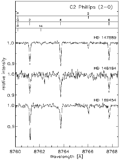
Figure 3: The comparison of intensities of few lines of the (2,0) band for 3 objects; the spectra were normalised to the line Q(4) 8763.74 Å (2,0) of HD 147889. The excitation temperatures $T_{06}$ of $C_{2}$ in HD 148184, HD 147889 and HD 169454 amount 74, 71 and 36 K, respectively.

4 Discussion

The $C_{2}$ molecule in interstellar clouds was observed many times, but usually measurements were limited to the most easily available to ground-based instruments lines of the (2,0) Phillips band. Apart from that measurements have usually been done with spectrographs of moderate resolution and signal-to-noise ratio (Snow, 1978; Hobbs, 1979; Danks & Lambert, 1983; van Dishoeck & de Zeeuw, 1984; Gredel & Muench, 1986; van Dishoeck & Black, 1989; Federman et al., 1994).

We measured absorption lines of the interstellar $C_{2}$ toward six reddened early type stars. The presence of $C_{2}$ in the sight line toward HD 76341 and HD 163800 has not been reported before.

Generally, excitation temperatures $T_{04}$ in our program stars tend to be above 47 K. One evident exception is HD 169454 (31 K). This cloud is definitely different from the others. There is the lowest gas kinetic temperature. Van Dishoeck & Black (1989) suggested that it is a real translucent cloud, whereas the other clouds are only diffuse interstellar clouds.

The behaviour of excitation temperatures may be seen directly by inspection of the portions of spectra around the Q(J”=4) transition of the (2,0) band (see Fig. 3). Note, that the spectrum was renormalized to the strength of Q(4) absorption. It is easily seen, that excitation temperature in HD 147889 is almost identical to that of HD 148184 and higher than the excitation temperature of HD 169454, which is confirmed in the quantitative analysis presented above.

Simultaneous observations of different vibrational bands give possibility to compare individually determined column densities for each band. For this purpose data collected for HD 147889 are especially useful. The observed column densities determined individually from bands (1,0), (2,0) and (3,0) amount $(11.2\pm 0.4)\times 10^{13}\mathrm{cm}^{-3}$, $(13.3\pm 0.2)\times 10^{13}\mathrm{cm}^{-3}$, and $(13.2\pm 0.8)\times 10^{13}\mathrm{cm}^{-3}$ respectively. The observed column density determined form all the bands together amounts $(13.0\pm 0.2)\times 10^{13}\mathrm{cm}^{-3}$. In conclusion, the determination of column densities from only one of these bands gives reasonable value of the $C_{2}$ column density; but the possibility of analysing lines of many different bands enhances the accuracy of the results. It excludes accidental errors (e.g. cosmic rays, telluric lines, instrumental errors) which are impossible to remove when only one band is available.

The interstellar absorption lines of $C_{2}$ toward HD 163800 arise in a single velocity component at a radial velocity, $V_{LSR}$ = 7.2 km s^-1 with respect to the local standard of rest. This radial velocity and position of the star suggest an association of the intervening molecular cloud with a large cloud of cold atomic hydrogen first surveyed by Riegel & Crutcher (1972) (Riegel-Crutcher cloud) as a prominent self-absorption feature in the 21 cm line. The distance to the cold atomic cloud is constrained by observations of optical lines in direction to background stars to be $125\pm 25$ pc (Crutcher & Lien, 1984a). Apparent association with atomic cloud does not imply physical connection with molecular cloud responsible for the observed absorptions of $C_{2}$. Small molecular cloud in the direction to HD 169454 is also possibly associated with the Riegel-Crutcher HI cloud; it was analysed by Jannuzi et al. (1988). The distance to HD 163800 from the spectroscopic data is estimated to be about 1.5 kpc.

The detailed comparison between our results and these of previous papers is shown in Appendix.

5 Summary

From the inspection of absorption lines in direction to HD 147889, we have found that individual Phillips bands (1,0), (2,0) and (3,0) give consistent results, both for column densities and excitation temperatures. However not every feature is the same easy to measure in all bands; e.g. the P(4) and Q(8) transitions are the easiest to separate in the (1,0) band and lines of R branch in (3,0) one (R-branch lines of the (2,0) band very often are located near to or in the wings of the stellar line HI what makes measurements uncertain). In this paper measurements of three Phillips bands were used to improve reliability of results due to growing number of identified lines and their separation.

The assumption of the identical radiation field for all clouds allows to calculate the density of collision partners $n_{c}$; the found values range from about 170 to 330 $\mathrm{cm}^{-3}$ (100 to 500 if errors are included). Absolute values may be different because of the peculiar radiation field and approximate treatment of the collisional excitation rate of $C_{2}$ with $H_{2}$. If the rotational population distributions are useful as diagnostic tools of the cloud densities, it is essential to have better understanding of cross sections of rotationally inelastic collisions of $C_{2}$ with $H_{2}$. Determination of $n_{c}$ is less dependent on the accurate value of the gas kinetic temperature. The visible transitions of $C_{2}$ are relatively easily observed, (in contrast to the far-UV bands of $H_{2}$ and very weak lines of $C_{3}$), and provide an important tool for the determination of the physical and chemical conditions of diffuse clouds.

The presence of $C_{2}$ in the measurable amount is reported for the two new lines of sight: toward HD 76341 and HD 163800. The latter star lies in the background of the Riegel-Crutcher cloud of the cold HI. The molecular cloud, origin of $C_{2}$ absorptions, may be physically associated with the atomic hydrogen cloud, similarly to the earlier considered small molecular cloud in direction to HD 169454 (Jannuzi et al., 1988).

To sum up, the high resolution and signal-to-noise ratio spectra acquired with the ESO instrument allow us to study densities and rotational temperatures varying from object to object with increasingly accuracy. This is seen particularly well when compare the theoretical model with the observational data (e.g. HD 147889 in Figure 2).

We are planning to continue the survey of high resolution and high signal-to-noise ratio spectra with detected interstellar diatomic carbon and compare with other interstellar absorption features. It is interesting whether other molecules are spatially correlated with $C_{2}$; this may efficiently constrain interstellar chemistry.

Appendix A

In this section detailed comparison between our results and those of previously published is demonstrated. $C_{2}$ in interstellar clouds towards HD 147889, HD 148184, HD 169454 and HD 179406 has already been observed, but towards HD 76341 and HD 163800 our determinations are the first ones. Comparison between our equivalent widths and data from literature is presented in Tables A2-A5. There are some differences between our results and those of previous papers which could be caused by different quality of the analysed spectra. We used the spectra from archival database collected by UVES, which are characterised by high resolving power ($\lambda/\Delta\lambda\sim 85,000$) and high signal-to-noise ratio ($S/N\sim 200$). The differences with published data may resemble the difficulty of measuring of weak lines.

In Table A1 there is a comparison between our results and those from previous papers.

Table 8: The comparison between our results and those from previous papers. Total column densities are rescaled to the value of $f_{20}$ used in this paper.

object	$T_{kin}^{a}[K]$	$T_{02}[K]$	$T_{04}[K]$	$T_{06}[K]$	$N_{col}[10^{13}\mathrm{cm}^{-2}]$	source
HD 147889	$70$				$8.3\pm 2.1$	van Dishoeck & de Zeeuw 1984
		$52\pm 22$	$116\pm 28$			Sonnentrucker et al. 2007b
	$39\pm 2$	$49\pm 7$	$62\pm 3$	$71\pm 2$	$13.3\pm 0.1$	this work
HD 148184	$40$		$65$		$3.0\pm 0.4$	van Dishoeck & de Zeeuw 1984
					$2.4$	Danks & Lambert 1983
	$50\pm 15$	$39\pm 16$	$57\pm 12$		$2.8\pm 0.3$	Sonnentrucker et al. 2007b
	$34\pm 12$	$82\pm 82$	$65\pm 12$	$74\pm 7$	$3.0\pm 0.3$	this work
HD 169454	$15$				$5.8$	Gredel & Muench 1986
	$15^{+}10\,-5$				$4.9\pm 1.0$	van Dishoeck & Black 1989
	$25$				$9.7$	Gredel 1999
	$20\pm 5$	$24\pm 6$	$37\pm 5$			Sonnentrucker et al. 2007c
	$19\pm 2$	$23\pm 3$	$31\pm 1$	$36\pm 1$	$6.5\pm 0.1$	this work
HD 179406	$55$			$66^{d}$	$3.7$	Federman & al. 1994
			$57\pm 11$		$5.0\pm 0.6^{f}$	Sonnentrucker et al. 2007e
	$38\pm 9$	$38\pm 12$	$59\pm 9$	$62\pm 5$	$3.9\pm 0.1$	this work
a gas kinetic temperature $T_{kin}$ is obtained form the best-fitting model.
b calculated by Sonnentrucker et al (2007) using the equivalent widths of Dishoeck & de Zeeuw(1984).
c calculated by Sonnentrucker et al (2007) using the equivalent widths of Gredel (1999).
d excitation temperature from all observed levels $T_{08}$
e calculated by Sonnentrucker et al (2007) using the equivalent widths of Federman et al. (1994).
f based on equivalent widths of Federman et al. 1994

The spectrum of HD 76341 was the most noisy in our sample, and thus the measurements are less reliable. We were able to assign 19 absorption features to the P, Q, R lines of the $C_{2}$ Phillips bands in total. There we found the lowest column density ($N_{col}=(1.1\pm 0.1)\,\times 10^{13}\mathrm{cm}^{-2}$) of $C_{2}$ in the whole sample.

In HD 147889 we measured the largest number of $C_{2}$ lines. Figure 1 shows portions of the spectrum HD 147889 (normalised to continuum, with removed telluric lines) with the assignment of the interstellar $C_{2}$ absorption lines. In total we were able to assign 68 absorption features to the P, Q, R lines of the $C_{2}$ Phillips bands. The computed column density $(13.3\pm 0.1)\times 10^{13}\mathrm{cm}^{-2}$ is the highest value of the sample.

In the case of HD 148184 we measured 40 absorption features belonging to the P, Q, R lines of the $C_{2}$ Phillips bands.

Toward HD 163800, in total we were able to assign 29 absorption features to the P, Q, R lines of the $C_{2}$ Phillips bands. We estimated $N_{col}=(2.8\pm 0.1)\times 10^{13}\mathrm{cm}^{-2}$.

For HD 169494 we were able to identify and measure 50 absorption lines of the P, Q, R branches of the $C_{2}$ Phillips bands. We estimated $N_{col}=(6.5\pm 0.1)\times 10^{13}\mathrm{cm}^{-2}$ and $n_{c}$ about $330\,\mathrm{cm}^{-3}$ (it is the highest value in our sample).

For HD 179406 we measured 36 absorption features to the P, Q, R lines of the $C_{2}$ Phillips bands.

Table 9: The comparison of our equivalent widths [mÅ] to data of van Dishoeck & de Zeeuw (1984) for HD 147889 of the (2,0) band.

$B(N^{\prime\prime})$	our results	D&Za
$R(6)$	$6.1\pm 0.3$	$4.0\pm 0.5$
$R(8)$	$3.6\pm 0.3$	$\leq 2.5$
$R(4)$	$9.2\pm 0.3$	$8.1\pm 0.4$
$R(10)$	$2.2\pm 0.3$
$R(2)$	$10.5\pm 0.3$	$5.3\pm 0.4$
$R(12)$	$1.8\pm 0.3$
$R(0)$	$7.5\pm 0.3$	$4.6\pm 0.2$
$Q(2)$	$12.7\pm 0.3$	$10.1\pm 0.6$
$Q(4)$	$13.1\pm 0.3$	$13.9\pm 1.2$
$P(2)$	$2.4\pm 0.3$	$2.9\pm 0.3$
$Q(6)$	$9.2\pm 0.3$	$7.8\pm 0.6$
$Q(8)$	$6.3\pm 0.3$	$4.9\pm 0.7$
$P(4)$	$4.7\pm 0.3$	$4.3\pm 0.3$
$Q(10)$	$4.5\pm 0.3$	$\leq 2.5$
$P(6)$	$5.1\pm 0.3$	$3.4\pm 0.3$
$Q(12)$	$2.3\pm 0.3$
$P(8)$	$2.4\pm 0.4$	$\leq 2.5$
$Q(14)$	$2.1\pm 0.3$
$P(10)$	$2.2\pm 0.3$
$Q(16)$	$2.2\pm 0.3$
$P(12)$	$0.8\pm 0.4$
$Q(18)$	$1.8\pm 0.5$u
$Q(20)$	$2.2\pm 0.7$u
$Q(22)$	$0.7\pm 0.4$u
$Q(26)$	$0.7\pm 0.5$u
a Measurements were made with coudé echelle spec-
trograph (with Reticon) which was fed by the 1.4-m
coudé auxiliary telescope at ESO, La Silla, Chile.
The resolving power in those observations was 80,000.
UVES allows to detect more transitions due to higher
resolution and S/N ratio.

Table 10: The comparison of our equivalent widths [mÅ] to data of van Dishoeck & de Zeeuw (1984) (D&Z) and Danks & Lambert (1983) (D&L) for HD 148184 of the (2,0) band.

$B(N^{\prime\prime})$	our results	D&Za	D&La
$R(6)$	$0.7\pm 0.4$	$1.3\pm 0.2$	0.96
$R(8)$	$0.6\pm 0.4$		0.81
$R(4)$	$1.5\pm 0.4$		0.44
$R(10)$	$0.7\pm 0.4$		0.48
$R(2)$	$2.7\pm 0.4$	$1.7\pm 0.2$	1.33
$R(12)$		$0.5\pm 0.2$
$R(0)$	$1.4\pm 0.4$u	$1.4\pm 0.1$	0.93
$Q(2)$	$3.0\pm 0.4$	$2.4\pm 0.1$	2.41
$R(14)$		$\leq 0.5$
$Q(4)$	$3.3\pm 0.5$	$2.5\pm 0.2$	2.15
$P(2)$	$0.5\pm 0.5$u	$\leq 0.5$
$Q(6)$	$3.4\pm 0.4$	$2.4\pm 0.2$	2.26
$R(16)$		$\leq 0.5$
$Q(8)$	$1.7\pm 0.4$	$2.0\pm 0.3$	1.67
$P(4)$	$1.4\pm 0.5$	$0.8\pm 0.2$	0.59
$Q(10)$	$1.0\pm 0.5$	$0.8\pm 0.2$	1.37
$P(6)$	$1.0\pm 0.4$	$1.0\pm 0.1$	0.67
$Q(12)$	$0.6\pm 0.4$	$0.9\pm 0.2$	0.78
$P(8)$		$1.0\pm 0.1$	0.89
$Q(14)$		$0.6\pm 0.1$	0.74
$P(10)$		$0.5\pm 0.2$	$\leq 0.67$
$Q(16)$	$0.8\pm 0.4$
a Measurements were made with coudé echelle spec-
trograph (with Reticon) which was fed by the 1.4-m
coudé auxiliary telescope at ESO, La Silla, Chile.
The resolving power in those observations was 80,000.

Table 11: The comparison of our equivalent widths [mÅ] to data of Federman et al. (1994) for HD 179406 of the (2,0) band.

$B(N^{\prime\prime})$	our results	Federmana
$R(6)$	$1.0\pm 0.5$	$3.0\pm 0.3$
$R(8)$	$0.4\pm 0.4$
$R(4)$	$2.7\pm 0.5$	$3.2\pm 0.2$
$R(2)$	$4.1\pm 0.5$	$5.0\pm 0.4$
$R(0)$	$3.3\pm 0.4$	$2.0\pm 0.2$
$Q(2)$	$4.7\pm 0.4$	$7.3\pm 0.5$
$R(14)$	$0.9\pm 0.3$u
$Q(4)$	$7.1\pm 0.5$u	$5.7\pm 0.5$
$P(2)$	$1.4\pm 0.4$	$\leq 1.1$
$Q(6)$	$3.6\pm 0.4$	$4.2\pm 0.4$
$Q(8)$	$1.3\pm 0.8$u	$1.1\pm 0.3^{b}$
$P(4)$	$0.9\pm 0.5$	$1.8\pm 0.3^{b}$
$Q(10)$	$2.2\pm 0.5$u
$P(6)$	$1.7\pm 0.5$u	$3.1\pm 0.6^{c}$
$Q(14)$	$0.6\pm 0.3$u
a Measurements were made with coudé spectrometer
which was on the 2.1-m telescope at McDonald
Observatory. The resolving power in those
observations typically was 25,000 to 30,000.
b $P(4)$ and $Q(8)$ lines are blended (Federman et al. 1994).
c Result is suspect because of possible stellar
contamination (Federman et al. 1994).

Table 12: The comparison of our equivalent widths [mÅ] to data of Gredel & Muench (1986) (G&M), van Dishoeck & Black (1989) (D&B) Crawford (1997) (Cr) and Gredel (1999) (G) for HD 169454 of the (2,0) band.

$B(N^{\prime\prime})$	our results	G&Ma	D&Ba	Crb	Gc
$R(6)$	$2.4\pm 0.3$				$\leq 2$
$R(8)$	$0.7\pm 0.3$				$\leq 1$
$R(4)$	$3.7\pm 0.3$	$3.8\pm 0.8$			$4.1\pm 1$
$R(10)$	$0.4\pm 0.3$u
$R(2)$	$8.1\pm 0.3$	$6.1\pm 1.2$	$6.0\pm 0.5$		$8.6\pm 1$
$R(12)$	$0.3\pm 0.2$
$R(0)$	$8.5\pm 0.3$	$8.2\pm 0.8$	$5.6\pm 1.0$	$6.23\pm 0.50$	$8.2\pm 1$
$Q(2)$	$10.3\pm 0.3$	$8.0\pm 1.6$	$6.6\pm 0.8$	$8.14\pm 1.18$	$10.3\pm 1$
$Q(4)$	$7.9\pm 0.3$	$5.0\pm 1.0$	$7.9\pm 0.7$	$3.98\pm 1.03$	$9.7\pm 1$
$P(2)$	$2.0\pm 0.3$	$2.3\pm 0.5$	$1.3\pm 0.3$	$2.82\pm 0.55$	$2.7\pm 2$
$Q(6)$	$3.0\pm 0.3$	$3.1\pm 0.6$	$3.9\pm 0.5$	$2.89\pm 0.59$	$3.8\pm 1$
$Q(8)$	$2.3\pm 0.3$	$2.6\pm 1.0$	$1.5\pm 0.5$	$1.28\pm 0.59$	$3.2\pm 1.5$
$P(4)$	$1.7\pm 0.3$	$2.0\pm 0.8$	$1.7\pm 0.8$	$1.68\pm 0.62$	$3.4\pm 1.5$
$Q(10)$	$0.8\pm 0.3$	$1.0\pm 0.5$	$1.0\pm 0.8$		$\leq 1$
$P(6)$	$0.9\pm 0.8$	$1.9\pm 0.8$	$<1.5$		$3.0\pm 1$
$Q(12)$	$1.0\pm 0.3$	$1.0\pm 0.5$	$<1.5$		$\leq 1$
$P(8)$	$0.8\pm 0.3$
$Q(14)$	$0.6\pm 0.4$
$Q(16)$	$0.6\pm 0.4$
a Measurements were made with coudé echelle spectrograph (with Reticon)
which was fed by the 1.4-m coudé auxiliary telescope at ESO, La Silla,
Chile. The resolving power in those observations was 80,000.
b The observations were obtained with the Ultra-High-Resolution Facility
(R = 910,000) at the Anglo-Australian Telescope
c The observations were made using the ESO New Technology Telescope,
La Silla, Chile, R$\sim$45,000.

References

- Bagnulo et al. (2003) Bagnulo S., Jehin E., Ledoux C., Cabanac R., Melo C., Gilmozzi R., The ESO Paranal Science Operations Team 2003, The Messenger, 114, 10
- Bakker et al. (1997) Bakker E. J., van Dishoeck E. F., Waters L. B. F. M., Schoenmaker T., 1997, A&A, 323, 469
- Bakker et al. (1996) Bakker E. J., Waters L. B. F. M., Lamers H. J. G. L. M., Trams N. R., van der Wolf F. L. A., 1996, A&A, 310, 893
- Ballik & Ramsay (1963) Ballik E. A., Ramsay D. A., 1963, ApJ, 137, 61
- Ballik & Ramsay (1963) Ballik E. A., Ramsay D. A., 1963, ApJ, 137, 64
- Black & Dalgarno (1977) Black J. H., Dalgarno A., 1977, ApJS, 34, 405
- Black et al. (1978) Black J. H., Hartquist T. W., Dalgarno A., 1978, ApJ, 224, 448
- Bondar et al. (2007) Bondar A., Kozak M., Gnaciński P., Galazutdinov G. A., Beletsky Y., Krełowski J., 2007, MNRAS, 378, 893
- Chaffee & Lutz (1978) Chaffee Jr. F. H., Lutz B. L., 1978, ApJ, 221, L91
- Chaffee et al. (1980) Chaffee Jr. F. H., Lutz B. L., Black J. H., Vanden Bout P. A., Snell R. L., 1980, ApJ, 236, 474
- Chauville et al. (1977) Chauville J., Maillard J. P., Mantz A. W., 1977, Journal of Molecular Spectroscopy, 68, 399
- Crawford (1997) Crawford I. A., 1997, MNRAS, 290, 41
- Crawford & Barlow (1996) Crawford I. A., Barlow M. J., 1996, MNRAS, 280, 863
- Crutcher (1985) Crutcher R. M., 1985, ApJ, 288, 604
- Crutcher & Chu (1985) Crutcher R. M., Chu Y.-H., 1985, ApJ, 290, 251
- Crutcher & Lien (1984a) Crutcher R. M., Lien D. J., 1984a, Technical report, Distances of local clouds from optical line observations
- Danks & Lambert (1983) Danks A. C., Lambert D. L., 1983, A&A, 124, 188
- Dekker et al. (2000) Dekker H., D’Odorico S., Kaufer A., Delabre B., Kotzlowski H., 2000, in M. Iye & A. F. Moorwood ed., Society of Photo-Optical Instrumentation Engineers (SPIE) Conference Series Vol. 4008 of Society of Photo-Optical Instrumentation Engineers (SPIE) Conference Series, Design, construction, and performance of UVES, the echelle spectrograph for the UT2 Kueyen Telescope at the ESO Paranal Observatory. pp 534–545
- Douay et al. (1988) Douay M., Nietmann R., Bernath P. F., 1988, Journal of Molecular Spectroscopy, 131, 261
- Douglas (1977) Douglas A. E., 1977, Nature, 269, 130
- Erman & Iwamae (1995) Erman P., Iwamae A., 1995, ApJ, 450, L31+
- Federman et al. (1994) Federman S. R., Strom C. J., Lambert D. L., Cardelli J. A., Smith V. V., Joseph C. L., 1994, ApJ, 424, 772
- Frisch (1972) Frisch P., 1972, ApJ, 173, 301
- Galazutdinov (1992) Galazutdinov G., 1992, Preprint Spets. Astrof. Obs. Russian, No. 92
- Gredel (1999) Gredel R., 1999, A&A, 351, 657
- Gredel & Muench (1986) Gredel R., Muench G., 1986, A&A, 154, 336
- Gredel et al. (1989) Gredel R., van Dishoeck E. F., Black J. H., 1989, ApJ, 338, 1047
- Gredel et al. (1991) Gredel R., van Dishoeck E. F., Black J. H., 1991, A&A, 251, 625
- Grevesse & Sauval (1973) Grevesse N., Sauval A. J., 1973, A&A, 27, 29
- Herbig & Leka (1991) Herbig G. H., Leka K. D., 1991, ApJ, 382, 193
- Hobbs (1979) Hobbs L. M., 1979, ApJ, 232, L175
- Hobbs et al. (2008) Hobbs L. M., York D. G., Snow T. P., Oka T., Thorburn J. A., Bishof M., Friedman S. D., McCall B. J., Rachford B., Sonnentrucker P., Welty D. E., 2008, ApJ, 680, 1256
- Hunter et al. (2006) Hunter I., Smoker J. V., Keenan F. P., Ledoux C., Jehin E., Cabanac R., Melo C., Bagnulo S., 2006, MNRAS, 367, 1478
- Jannuzi et al. (1988) Jannuzi B. T., Black J. H., Lada C. J., van Dishoeck E. F., 1988, ApJ, 332, 995
- Johnson et al. (1983) Johnson J. R., Fink U., Larson H. P., 1983, ApJ, 270, 769
- Kaźmierczak et al. (2009) Kaźmierczak M., Gnaciński P., Schmidt M. R., Galazutdinov G., Bondar A., Krełowski J., 2009, A&A, 498, 785
- Lambert (1978) Lambert D. L., 1978, MNRAS, 182, 249
- Lambert & Danks (1983) Lambert D. L., Danks A. C., 1983, ApJ, 268, 428
- Lambert et al. (1995) Lambert D. L., Sheffer Y., Federman S. R., 1995, ApJ, 438, 740
- Langhoff et al. (1990) Langhoff S. R., Bauschlicher Jr. C. W., Rendell A. P., Komornicki A., 1990, J. Chem. Phys., 92, 6599
- Lien (1984) Lien D. J., 1984, ApJ, 287, L95
- Marenin & Johnson (1970) Marenin I. R., Johnson H. R., 1970, Journal of Quantitative Spectroscopy and Radiative Transfer, 10, 305
- Mayer & O’dell (1968) Mayer P., O’dell C. R., 1968, ApJ, 153, 951
- Morton (1991) Morton D. C., 1991, ApJS, 77, 119
- Querci et al. (1971) Querci F., Querci M., Kunde V. G., 1971, A&A, 15, 256
- Riegel & Crutcher (1972) Riegel K. W., Crutcher R. M., 1972, A&A, 18, 55
- Snow (1978) Snow Jr. T. P., 1978, ApJ, 220, L93