The inner structure of very massive elliptical galaxies: implications for the inside-out formation mechanism of galaxies
Abstract
We analyze a sample of 23 supermassive elliptical galaxies (central velocity dispersion larger than 330 km s-1), drawn from the SDSS. For each object, we estimate the dynamical mass from the light profile and central velocity dispersion, and compare it with the stellar mass derived from stellar population models. We show that these galaxies are dominated by luminous matter within the radius for which the velocity dispersion is measured. We find that the sizes and stellar masses are tightly correlated, with , making the mean density within the de Vaucouleurs radius a steeply declining function of : . These scalings are easily derived from the virial theorem if one recalls that this sample has essentially fixed (but large) . In contrast, the mean density within 1 kpc is almost independent of , at a value that is in good agreement with recent studies of galaxies. The fact that the mass within 1 kpc has remained approximately unchanged suggests assembly histories that were dominated by minor mergers – but we discuss why this is not the unique way to achieve this. Moreover, the total stellar mass of the objects in our sample is typically a factor of larger than that in the high redshift () sample, an amount which seems difficult to achieve. If our galaxies are the evolved objects of the recent high redshift studies, then we suggest that major mergers were required at , and that minor mergers become the dominant growth mechanism for massive galaxies at .
keywords:
galaxies: formation – galaxies: evolution – galaxies: elliptical and lenticular, cD – galaxies: high-redshift.1 Introduction
The study of luminous and dark matter in elliptical galaxies is crucial to understanding the formation of massive galaxies in our Universe. In hierarchical models, ellipticals are the result of interactions and mergers of spiral galaxies (e.g. Blumenthal et al. 1984). This is in contrast to a scenario in which they form from a monolithic collapse (e.g. Eggen et al. 1962; Granato et al. 2004). The most massive elliptical galaxies, with baryonic masses , are challenging because they should have formed in the very early universe and at the same time undergone a large deal of merging.
There is now growing evidence that massive galaxies ( M⊙) did exist at . Some work suggests that they were much smaller and denser than their local counterparts of the same stellar mass (e.g. Trujillo et al. 2006; van Dokkum et al. 2008; Cimatti et al. 2008; Saracco et al. 2009) and that similar compact galaxies to those observed at high-redshift do not exist in the local universe (e.g. Trujillo et al. 2009). These results raised the question of what process or processes have acted to increase the sizes of these objects to make them consistent with the larger sizes we see at late times (e.g. van Dokkum et al. 2008; Fan et al. 2008).
Bezanson et al. (2009) showed that the stellar density within the central 1 kpc of ellipticals at is similar to that for nearby ellipticals (they differ by only a factor of , compared to a difference of a factor of if the comparison is done within the half-light radius). This suggests an inside-out, hierarchical growth scenario dominated by dry minor mergers which add mass primarily to the outer regions (e.g. Loeb & Peebles 2003; Bournaud et al. 2007; Naab et al. 2007; Hopkins et al. 2009).
However, the evidence for small sizes at high-redshift and the lack of such objects at low-redshift is not uncontested. For example, Mancini et al. (2010) have argued that neglect of low surface brightness features will bias to small values. Their analysis shows that some of the objects at are not small for their compared to objects. A similar result was recently presented by Onodera et al. (2010) who found a analog of local ultra-massive elliptical galaxies. Recently, Saracco et al. (2010) found from a complete sample of 34 early-type galaxies at that 21 of these are similar to the local ones even though they are co-eval with more compact early-type galaxies. In addition, Valentinuzzi et al. (2010) found that about 25% of the objects with M⊙ in local clusters are superdense (i.e. they have sizes like those observed out to z ). However, they found that there is strong evidence for a large evolution in radius for the most massive galaxies, i.e. BCGs ( M⊙).
Indeed, evolution in the properties of local BCGs was detected by Bernardi (2009), who showed that the sizes and velocity dispersions of BCGs (and of massive early-type galaxies) in the local Universe () are still evolving. This work suggests that minor dry mergers dominate the assembling of BCGs at lower redshifts since the observed size evolution is more rapid than expected by major dry mergers once one accounts for the small changes in the observed luminosity/mass functions (% since ; e.g. Wake et al. 2006; Brown et al. 2007; Cool et al. 2008). Minor dry mergers are better able to reconcile the observations of size evolution with little mass evolution. In addition, Bernardi (2009) also claims that minor mergers can also help to reconcile the substantial growth ( a factor of 2) predicted for the dark matter halos since (e.g. Sheth & Tormen 1999) with the little stellar mass evolution in the central galaxies (i.e. %): indeed, the fractional mass growth of BCGs need not be the same as that of their host clusters – some of the added stellar mass must make the intercluster light.
However, while an inside-out, hierarchical growth scenario dominated by minor dry mergers can describe the assembling of BCGs at low redshift, the recent analysis of Bernardi et al. (2010b) suggests that some of the features observed in the scaling relations of massive early-type galaxies at (e.g. the upwards curvature in the color relation, the decrease in the mean axis ratio and color gradients and the fact that most scaling relations with are well-described by a single power law) can only be explained by an assembly history dominated by major dry mergers above this mass.
The main goal of this paper is to use both visible stellar masses and dynamical stellar masses, for 23 supermassive elliptical galaxies identified by Bernardi et al. (2006, 2008), to investigate these issues in the light of previous work.
The paper is organized as follows. We describe the observables in Section 2, our procedure for estimating the total dynamical masses, and the fraction which is in stars, in Section 3, a comparison of these dynamical mass estimates with those from stellar population models in Section 4, and scaling relations between size and mass in Section 5. A final section discusses our findings: we argue that it is not clear that minor mergers since can have been the dominant formation mechanism of these massive galaxies.
When necessary, we assume a flat background cosmology that is dominated by a cosmological constant at the present time: , , and we set Hubble’s constant to km s-1Mpc-1.
| # | r | r | rap | ||
|---|---|---|---|---|---|
| (km s-1) | (kpc) | (kpc) | (kpc) | ||
| 1 | 339 | 8.5 | 19.031 | 5.698 | 7.5 |
| 2 | 346 | 6.1 | 18.775 | 7.326 | 6.2 |
| 3 | 353 | 12.8 | 10.923 | 3.690 | 5.2 |
| 4 | 352 | 20.2 | 21.228 | 4.107 | 10.2 |
| 5 | 356 | 16.9 | 13.907 | 3.366 | 8.7 |
| 6 | 350 | 6.5 | 8.295 | 4.491 | 6.7 |
| 7 | 361 | 26.1 | 16.345 | 2.921 | 8.2 |
| 8 | 356 | 11.9 | 10.228 | 3.628 | 7.7 |
| 9 | 355 | 7.7 | 9.999 | 4.675 | 6.4 |
| 10 | 351 | 3.9 | 4.053 | 4.234 | 7.1 |
| 11 | 356 | 5.3 | 6.360 | 4.401 | 5.0 |
| 12 | 346 | 2.2 | 4.562 | 6.591 | 4.8 |
| 13 | 368 | 16.2 | 17.004 | 4.136 | 8.2 |
| 14 | 364 | 10.9 | 16.622 | 5.194 | 7.2 |
| 15 | 356 | 5.1 | 7.723 | 4.986 | 6.8 |
| 16 | 364 | 7.4 | 18.976 | 5.988 | 8.9 |
| 17 | 362 | 2.2 | 5.579 | 6.573 | 4.0 |
| 18 | 382 | 12.9 | 18.487 | 4.825 | 8.4 |
| 19 | 369 | 1.8 | 4.143 | 7.349 | 3.6 |
| 20 | 370 | 2.6 | 4.882 | 5.491 | 5.0 |
| 21 | 390 | 11.2 | 29.410 | 6.422 | 9.3 |
| 22 | 392 | 2.8 | 8.089 | 6.738 | 4.2 |
| 23 | 412 | 29.4 | 15.150 | 2.756 | 7.8 |
2 Observational properties of giant ellipticals
We use the sample of 23, , supermassive elliptical galaxies, selected by Bernardi et al. (2006, 2008) from the SDSS database on the basis of their large velocity dispersions: 330 km s-1. Surface brightness fits and analyses of the SDSS and HST-based light profiles are presented in Hyde et al. (2008). An overview of the galaxy properties that we need for this study is gathered in Table 1.
For all the objects in our sample, the observed surface brightness distribution was fit to de Vaucouleurs (DeV) and Sersic (S) profiles:
| (1) |
| (2) |
where and are the central surface brightness and the projected half-light radius ( is given Table 1). (We use the parameters provided by Hyde et al. 2008, rather than those output from the SDSS database. Hyde et al. also provide fits to Bulge/Disk decompositions, which we do not use here.) We use to denote the mass-to-light ratio, and we define the surface mass density , then the deprojected density, computed by inverting the Abel equation, is
| (3) |
The mass within (a sphere of radius) is
| (4) |
Note that we could have defined the analogous quantities for the light, then and . The quantity of most interest in this paper is the total stellar mass: . We describe how we estimate it in the next section.
The other observed quantity is the average velocity dispersion within the SDSS fiber, which has a diameter (2) of 3 arcsec, that corresponds to about 5-10 kpc according to the distance of our galaxies. (Note that here we do not use aperture corrected to reported by Bernardi et al. 2006, 2008.) The value of is related to the line-of-sight velocity dispersion of the object, weighted by the surface-brightness profile:
| (5) |
where and is the velocity dispersion at projected distance from the center.
The quantity is related to the gravitational potential, and hence to the total mass of the system, as follows.
3 Jeans’ equation analysis
In what follows, we provide an estimate of the total mass, and the fraction of this which is in stars, for the objects in our sample. Our analysis assumes that the objects – both the stellar and the dark matter components – are spherical, with constant stellar mass-to-light ratios, and no anisotropic velocities. This is extremely idealized: Bernardi et al. (2008) have argued that many of these objects are likely to be prolate objects viewed along the long axis. We discuss this more complex case in an Appendix, but since none of our conclusions are sensitive to this, we have kept the simpler (spherical, isotropic) model in the main body of the text. Bernardi et al. also argue that some of these objects may be rotating – an effect we do not include in our analysis. We have not removed such objects from our analysis, since it is interesting that they appear to show similar scalings as the objects which are not rotating.
3.1 Spherical symmetry and isotropic velocities
The 1-D Jeans equation in spherical symmetry (Binney & Tremaine 1987) relates the radial velocity dispersion to the mass distribution:
| (6) |
where is the density of the stellar component at , is the total mass () within and is the anisotropy profile. Studies of nearby elliptical galaxies indicate that the tangential anisotropy within the half-light radius is negligible (e.g. Matthias & Gerhard 1999; Gerhard et al. 2001; Koopmans & Treu 2003; Koopmans et al. 2009). Therefore we set in what follows – the Appendix shows how our results are modified if . Thus, equation (6) implies
| (7) |
An observer only measures the projection along the line of sight, , which is given by
| (8) |
Inserting equation (7) in (8), and this in (5) shows how the total dynamical mass is related to the observed light profile and .
3.2 Insignificance of dark matter in
In what follows, we estimate the total mass within some radius as the sum of the stellar mass (obtained from the observed light profile with the assumption of constant mass-to-light ratio) and that of the dark matter, for which we use the fitting formula of Navarro et al. (1996; hereafter NFW).
For an NFW profile with total mass , the virial radius is
| (9) |
The mass within some is given by
| (10) |
where : is a characteristic scale length for the halo, and the final equality defines the concentration parameter
| (11) |
Note that massive halos are less concentrated. For small ,
| (12) |
for , this is .
We model the total mass of each galaxy in our sample as a superposition of the deprojected de Vaucouleurs or Sersic profile having total mass and an NFW halo with a total mass . This represents a compromise: adiabatic contraction arguments suggest that the dark matter should become more centrally concentrated than a pure NFW profile, as the gas which formed the stellar component shrinks towards the center – we are ignoring this effect (see Padmanabhan et al. 2004; Schulz et al. 2010; Treu et al. 2010 for recent analyses of other samples in which this effect is included). On the other hand, observations suggest that galaxies have a cored rather than a cuspy halo (e.g. Salucci et al. 2007) – even an uncontracted NFW profile is too steep.
| # | |||||
|---|---|---|---|---|---|
| () | (M⊙) | (M⊙) | (M⊙) | (M⊙) | |
| 1 | 5 | 9.5 | 11.2 | 5.5 | 8.5 |
| 2 | 3 | 7.6 | 8.3 | 7.4 | 13.2 |
| 3 | 5 | 15.0 | 14.4 | 14.5 | 13.2 |
| 4 | 8 | 21.7 | 22.1 | 11.7 | 12.3 |
| 5 | 6 | 19.7 | 19.6 | 14.5 | 12.6 |
| 6 | 2 | 8.3 | 9.0 | 23.4 | 26.9 |
| 7 | 10 | 28.7 | 25.6 | 24.0 | 18.2 |
| 8 | 5 | 14.5 | 14.1 | 6.6 | 6.0 |
| 9 | 4 | 9.7 | 10.3 | 5.2 | 6.0 |
| 10 | 1 | 5.2 | 5.2 | 7.9 | 7.9 |
| 11 | 2 | 6.9 | 7.3 | 2.2 | 2.4 |
| 12 | 1 | 3.0 | 3.1 | 2.6 | 3.6 |
| 13 | 6 | 20.4 | 20.7 | 10.0 | 10.2 |
| 14 | 4 | 14.2 | 15.0 | 18.2 | 22.9 |
| 15 | 3 | 6.8 | 7.5 | 3.4 | 4.3 |
| 16 | 3 | 10.1 | 12.4 | 6.6 | 11.0 |
| 17 | 2 | 3.1 | 3.6 | 0.9 | 1.4 |
| 18 | 5 | 18.1 | 19.6 | 8.1 | 10.0 |
| 19 | 1 | 2.7 | 2.7 | 2.9 | 3.6 |
| 20 | 1 | 4.0 | 4.6 | 6.9 | 9.5 |
| 21 | 3 | 17.3 | 19.8 | 25.7 | 42.7 |
| 22 | 1 | 4.7 | 5.7 | 7.1 | 12.3 |
To proceed further, we assume that :
| (13) |
following Shankar et al. (2006). This makes
| (14) |
Notice that big galaxies are likely to have some scatter around this number (i.e. 30). In fact for smaller values, our conclusion that the stars dominate the mass will be stronger. We demonstrate that the mass within is dominated by the stars, not the dark matter. For , kpc, and the NFW mass within is approximately , whereas the stellar mass within is slightly less than . Since , the total mass within is dominated by the stellar mass. Consequently, is also dominated by the stellar mass.
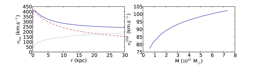
We show this explicitly in Figure 1. The left hand panel shows , obtained from equation 7, 8, for an elliptical galaxy with and kpc. We see that the contribution from the dark matter component is always much smaller than that of the stellar component ().
Then we show that is always negligible compared to observed (right hand panel). Since , within our assumptions, the measured value of provides a good estimate of , without being contaminated by the dark matter component. The effect of DM is small, we can evaluate it and correct the estimation of by assuming equation 13. On average the dark matter component contributes to less than to the total velocity dispersion (Table 2).
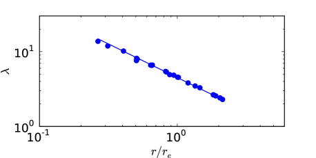
Now we build a new stellar mass estimator that exploits the quantity . The Jeans equation implies that the quantity should be proportional to a function of . If we set
| (15) |
the actual value of plotted in Figure 2 can be fitted by:
| (16) |
As a check, note that if the power-law above had slope , then ; this is the scaling that is usually assumed. The zero-point of the relation, 4.5, is close to that commonly assumed for a pure de Vaucouleurs profile (e.g. Bernardi et al. 2010a). It is also close to that derived from analyses which assume adiabatic contraction (Padmanabhan et al. 2004).
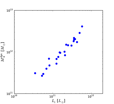
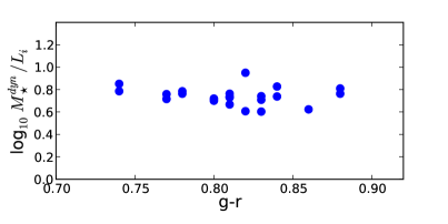
The top panel of Figure 3 shows the dynamical stellar mass computed as described above, versus the luminosity in the i-band. The bottom panel shows the corresponding mass-to-light ratio versus color (g-r).
4 Comparison with stellar mass estimates from photometry
We estimate the stellar masses , from the stellar population (hereafter SP) model of Maraston et al. (2009) (available at www.maraston.eu). This is a two-component model made by a major metal-rich population and a low percentage () of an old and metal-poor population with the same age. Moreover, an improvement in the spectra of K-giants is included through the empirical stellar spectra of Pickles (1998). The initial mass function in the Maraston et al. (2009) paper was a Salpeter (1955) and we did not modify this assumption here. We use these models because they trace the color evolution of Luminous Red Galaxies (LRGs) in SDSS from redshift 0.1 to 0.6 much better than previous attempts did (see Maraston et al. 2009).
We obtain the stellar masses through Spectral Energy Distribution (SED) fitting, as in Maraston et al. (2006), e.g., by using the Maraston et al. 2009 templates in the Hyper-Z code (Bolzonella et al. 2000)111We checked that had we fitted a composite model with identical characteristics, but obtained with the Maraston (2005) SP models, i.e. the standard models based on the Kurucz (1979) model atmospheres, we would have obtained the same results.. We computed the stellar masses using both de Vaucouleurs and Sersic magnitudes. The first set were obtained by fitting the ugriz de Vaucouleurs magnitudes available from the SDSS database, while the second set was computed rescaling the SDSS de Vaucouleurs magnitudes by the difference between the i-band Sersic and de Vaucouleurs magnitude observed by Hyde et al. (2008). This is a good approximation since color gradients are small.
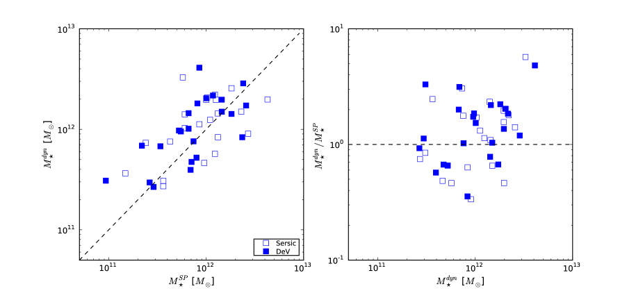
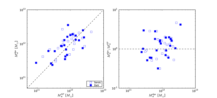
The panel on the left of Figure 4 shows our estimates versus those from the stellar population model. Note that , the stellar masses as obtained with these composite models are in agreement with the dynamical masses.
5 Structural properties of giant ellipticals
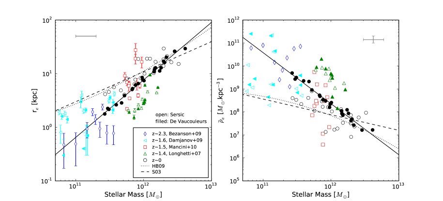
We now analyze the correlation between size and mass in our objects. The left hand panel of Figure 5 shows the correlation between and using our dynamical estimates of . The solid line shows the direct fit (i.e. )
| (17) |
This relation is significantly steeper than the that is usually reported (e.g. Hyde & Bernardi 2009). However, if we recall that these objects all have large , then the relevant comparison is to the relation at fixed and . This slope is close to 0.9 (Bernardi et al. 2008). In this case, it is plausible that our (now only slightly) steeper slope is due to the fact that our estimator is less noisy.
In fact, the small scatter in our relation can also be understood in these terms. Equations (15) and (16) show that our dynamical estimate of is proportional to . Figure 2 shows that there is little scatter around this relation. However, our sample has essentially fixed , and has only a small scatter, so Figure 5 is almost a plot of vs , with the zero-point being set by the mean and values in the sample. This is why the slope is close to unity. Of course, if the stellar distribution were not homologous, or the dark matter was a significant fraction of the total mass, then need not have small scatter.
The diamonds, squares, triangles show these same relations, but now obtained from a sample of objects by Bezanson et al. (2009), Damjanov et al. (2009), Mancini et al. (2010) and Longhetti et al. (2007), respectively. A number of studies have noted that the objects are significantly smaller than objects of the same (dotted or dashed curves). Note that Bezanson et al., Mancini et al., Longhetti et al. and Damjanov et al. computed their stellar masses with different IMF (Kroupa, Chabrier, Salpeter and Baldry & Glazebrook) and different stellar population models (Bruzual & Charlot 2003 and Maraston 2005). The fit from Hyde & Bernardi (2009) and Shen et al. (2003) were computed using a Chabrier IMF. In order to compare these different samples we recalibrated the masses to a Salpeter IMF (as used in Maraston et al. 2009) using these scale-factors: . In addition, to account for differences in stellar population models we rescaled the Bezanson et al. data multiplying their stellar masses by 0.7 (as e.g. in Mancini et al. 2010, see also Muzzin et al. 2009) and by 0.5 for the Damjanov et al. stellar masses.
The evidence for small sizes at is not uncontested. Mancini et al. (2010) have argued that neglect of low surface brightness features will bias to small values (while the bias in is small – C. Mancini private communication). Accounting for this effect in a sample at yields the open squares in Figure 5. Evidently, these objects are not small for their compared to objects. If both Mancini et al. and Bezanson et al. are correct, and both probe the massive end of the population at their respective mean redshifts, then there must have been significant evolution in size and stellar mass between and .
In view of this discussion, it is remarkable that the compact galaxies appear to trace the small size and end of the relation we find at , for fixed (solid line). The sample of Mancini et al. (2010) is confined to a narrower range of , making it difficult to define a relation. However, at this , the difference between the solid line km s-1) and the others (bulk of early-type population) is a factor of two or less. It will be interesting if future measurements show the objects to have km s-1, and even more so if this is also true for the most compact of the objects in the Mancini et al. sample.
We now turn to a slightly different version of the correlation between size and mass, namely that between average density and mass. For this purpose, it is useful to define
| (18) |
the average density within . In what follows, we will pay special attention to and : the mean density within the de Vaucouleurs radius , and within 1 kpc, respectively. Whereas can be thought of as a characteristic density, is more like the central density (recall that, for this sample, kpc).
The right-hand panel of Figure 6 shows the correlation between and , using the same format as for the panel on the left. Fitting to the relation defined by our dynamically estimated yields
| (19) |
This characteristic density is a sharply declining function of stellar mass – the decline is significantly steeper than previously reported for a sample which includes the full range of early-types (e.g. Bernardi et al. 2003; Hyde & Bernardi 2009). Following our discussion of the relation above, the more relevant comparison may be with the relation at fixed , for which the slope is (Bernardi et al. 2008). Our current estimate is slightly steeper, perhaps because our mass estimate is less noisy. To see this, note that we could have derived the slope from the fact that , where the final expression uses the fact that the scatter between and is small (which we argued was a consequence of the fact that our sample has only a small range of , a small range in , and that Figure 2 has small scatter). We note that, while the objects have orders of magnitude larger than the bulk of the objects of the same (compare diamonds with dashed or dotted curves), they are only slightly denser than objects of the same , if such objects had km s-1 (extrapolate solid line to small ).
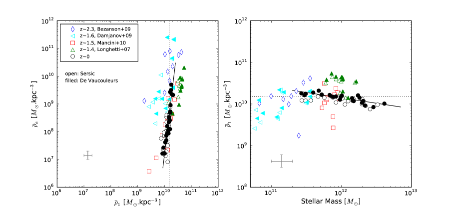
The steepness of this relation stands in stark contrast to the relation between and . The right-hand panel of Figure 6 shows that this relation is very shallow. We find
| (20) |
While the mass varies by 2 orders of magnitude (from to ), the central density remains constant at about .
The left-hand panel of Figure 6 shows another way of presenting this information: while varies by 3 orders of magnitude, varies by less than a factor of 2. We find
| (21) |
Thus the central density is approximately constant for all the galaxies of our sample.
It is quite remarkable that they show the same relation as in the samples of Mancini et al. and Longhetti et al. at as well as of Bezanson et al. (2009) at . Although is orders of magnitude larger in the sample than at , is different by only a factor of two or so.
6 Discussion and conclusions
We analyzed a sample of 23 giant elliptical galaxies. They are very massive () with large central velocity dispersions km s-1, which suggests old stellar populations (Bernardi et al. 2005). We estimated dynamical masses for each of these systems by using the observed light profiles and central velocity dispersions, by solving the Jeans Equation, under the assumptions of spherical symmetry, no tangential velocity dispersions, no radial dependence of the stellar mass-to-light ratio, and that each system has 30 times more dark matter than stellar matter within the virial radius, with the dark matter following an NFW profile (i.e. no accounting for adiabatic contraction).
We found that the total stellar masses of these systems vary from about to (Table 2). In such models, the contribution of the dark matter modifies the central velocity dispersion by less than (Figure 1). Thus, for these objects, the observed provides a good estimator of the luminous mass (equation 16). We compared the masses we derive to estimates of the stellar mass from stellar population models (Figure 4). We find good agreement using a composite model with high age and a small (by mass) metal-poor sub-component. This model fits well the colors of Luminous Red Galaxies in SDSS. A major result of this study is that we compute the mass-to-light ratio for massive elliptical galaxies. This ratio is roughly constant for all the sample (Figure 3), we find in the i-band, for .
We also studied different ways of presenting the correlation between size and mass (Figure 5). The correlation we find, , is slightly steeper than that reported by Bernardi et al. (2008). We suggest that this is because our estimate of is less noisy. For similar reasons, we find that the density within is a more strongly decreasing function of than reported by Bernardi et al. (2008). We find compared to their .
A notable result is that galaxies at z 2.3 (Bezanson et al.) and z 1.5 (Mancini et al.) appear to follow the same relation that we find at z 0. If each sample correctly gather the most massive galaxies for each range of redshift, the evolution between the size and the stellar mass should be meaningful.
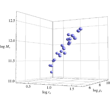
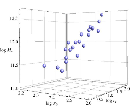
The small scatter associated with our dynamical estimator of means that, in the space of , and , the objects in our sample trace out a one-dimensional curve (although we have argued, as did Bernardi et al. 2008, that the scaling we find is consistent with the simplest virial theorem scaling, once we account for the fact that these objects have essentially fixed ). This is also true in the space of , and . We show this explicitly in Figure 7. Had we used the stellar population-based estimate of , these curves would have been broadened into a plane. Since the () projection is similar to that of the Fundamental Plane, our results suggest that scatter in the relation between and , or uncertainties in estimating serve to enhance the impression of a plane rather than a curve.
On the other hand, some of the decreased scatter in our analysis is due to our neglect of anisotropic velocity dispersion profiles. We explore this in the Appendix. Nevertheless, it is likely that the scaling relation between and of giant ellipticals is significantly steeper than for spirals (which have ). Understanding why is a challenge for models in which ellipticals form from mergers of spirals.
Although decreases strongly with , the average density on smaller scales (we chose 1 kpc) is almost independent of (Figure 6). Moreover, it is remarkably similar to that found by Bezanson et al. (2009), in their analysis of galaxies. The mean density within 1 kpc seems to be independent of the redshift and of the mass on an object by object basis. I.e., since , as these galaxies grew in mass, the mass in the inner kpc remained unchanged. Understanding why is an interesting challenge.
Although this is most easily accomplished in models where the mass is added to the outer regions only (e.g. Lapi & Cavaliere 2009, Cook et al 2009) – so it is tempting to conclude that minor mergers were the dominant growth mode since (e.g. Bezanson et al. 2009) – there is a direct counterexample to this conclusion in the literature. In numerical simulations of hierarchical structure formation, Gao et al. (2004) find that although the mass in the central regions of what becomes a massive cluster at has remained constant since , the particles which make up this mass changed dramatically as the objects assembled. This assembly occurred through a sequence of major mergers at ; with minor mergers beginning to dominate the mass growth only at . Note that in hierarchical models, what is true for cluster mass halos is also true for galaxy mass halos. While gastrophysics may complicate the discussion, we raise this as an example where mass growth due to major mergers does not lead to increased density in the central regions. This appears to be in remarkable agreement with what we see. If the objects studied by Bezanson et al. (2009) are to evolve into the objects in our sample, then the required mass growth is about a factor of 5 (Figure 6) – this is larger than most minor merger models can accommodate. It may well be that major mergers were required at and that minor mergers become the dominant growth mechanism for massive galaxies only at lower redshift (Bernardi 2009; Bernardi et al. 2010b).
Our Figure 5 supports such a picture: major mergers would move the objects approximately parallel to the solid lines in the two panels. A factor of 5 change in mass and size would bring them into much better agreement with the dotted and dashed relations in the panel on the left, but they would still lie slightly above the corresponding line in the panel on the right. Subsequent minor mergers would increase the sizes and decrease the velocity dispersions, bringing both the sizes and densities into even better agreement. (Note that a small fractional increase in mass results in a larger fractional increase in size and an even larger fractional decrease in density. Indeed, because density is proportional to , minor mergers are a great way to decrease the density for a modest change in mass.) If the high redshift objects indeed have km s-1 (as our Figure 5 may suggest), the decrease in associated with minor mergers will (in fact, may be required to) bring the number density of large objects into better agreement with that seen locally (Sheth et al. 2003).
On the other hand, selection effects (e.g. due to the small volume observed) could limit the detection of these very massive galaxies. For example, the sample of ultramassive early-type galaxies of Mancini et al. (2010) is selected from a 2 deg2 field. In such a volume, if galaxies of M M⊙ are yet present at , as predicted by model like Fan et al. (2010), the number of detections should be around unity and therefore not necessary detected. The detection of these massive objects (already difficult in the local universe) is thus a challenge for the high redshift universe.
Acknowledgments
We thank L. Danese, C. Mancini R. Sheth and P. van Dokkum for helpful discussions and the anonymous referee for comments that have improved the presentation of our results. M.B. is grateful for support provided by NASA grant ADP/NNX09AD02G. CM and JP acknowledge support from the Marie Curie Excellence Team Grant ’Unimass’, ref. MEXT-CT-2006-042754, of the European Community.
Funding for the Sloan Digital Sky Survey (SDSS) and SDSS-II Archive has been provided by the Alfred P. Sloan Foundation, the Participating Institutions, the National Science Foundation, the U.S. Department of Energy, the National Aeronautics and Space Administration, the Japanese Monbukagakusho, and the Max Planck Society, and the Higher Education Funding Council for England. The SDSS Web site is http://www.sdss.org/.
The SDSS is managed by the Astrophysical Research Consortium (ARC) for the Participating Institutions. The Participating Institutions are the American Museum of Natural History, Astrophysical Institute Potsdam, University of Basel, University of Cambridge, Case Western Reserve University, The University of Chicago, Drexel University, Fermilab, the Institute for Advanced Study, the Japan Participation Group, The Johns Hopkins University, the Joint Institute for Nuclear Astrophysics, the Kavli Institute for Particle Astrophysics and Cosmology, the Korean Scientist Group, the Chinese Academy of Sciences (LAMOST), Los Alamos National Laboratory, the Max-Planck-Institute for Astronomy (MPIA), the Max-Planck-Institute for Astrophysics (MPA), New Mexico State University, Ohio State University, University of Pittsburgh, University of Portsmouth, Princeton University, the United States Naval Observatory, and the University of Washington.
References
- [1] Bernardi, M., Sheth, R. K., Annis, J. et al. 2003, AJ, 125, 1849
- [2] Bernardi, M., Sheth, R. K., Nichol, R. C., Schneider, D. P. & Brinkmann, J. 2005, AJ, 129, 61
- [3] Bernardi M., Sheth R. K., Nichol R. C., Miller C. J., Schlegel D., Frieman J., Schneider D. P., Subbarao M., York D. G., Brinkmann J., 2006, AJ, 131, 2018
- [4] Bernardi M., Hyde J. B., Fritz A., Sheth R. K., Gebhardt K., Nichol R. C., 2008, MNRAS, 391, 1191
- [5] Bernardi, M. 2009, MNRAS, 395, 1491
- [6] Bernardi, M., Shankar, F., Hyde, J. B., Mei, S., Marulli, F. & Sheth, R. K. 2010a, MNRAS, in press (arXiv:0910.1093)
- [7] Bernardi, M., Roche, N., Shankar, F. & Sheth, R. 2010b, MNRAS, submitted (arXiv:1005.3770)
- [8] Bezanson R., van Dokkum P. G., Tal T., Marchesini D., Kriek M.,Franx M., Coppi P., 2009, ApJ, 697, 1290
- [9] Binney J., Mamon G. A., 1982, MNRAS, 200, 361
- [10] Binney J., Tremaine S., Princeton University Press, 1987, 747
- [11] Blumenthal G. R., Faber S. M., Primack J. R., Rees M. J.: 1984 Nature, 311, 517
- [12] Bolzonella M., Miralles J.-M., Pello R., 2000, A&A, 363, 476
- [13] Bournaud, F., Jog. C. J. & Combes, F. 2007, A&A, 476, 1179
- [14] Brown, M. J. I., Dey, A., Jannuzi, B. T., Brand, K., Benson, A. J., Brodwin, M., Croton, D. J., & Eisenhardt, P. R. 2007, ApJ, 654, 858
- [15] Bruzual G., Charlot S., 2003, MNRAS, 344, 1000
- [16] Cimatti, A., et al. 2008, A&A, 482, 21
- [17] Cook M., Lapi A., Granato G. L., 2009, MNRAS, 397, 534
- [18] Cool, R. J., et al. 2008, ApJ, 682, 919
- [19] Damjanov I., McCarthy P. J., Abraham R. G., Glazebrook K., Yan H. et al. 2009, ApJ, 695, 101
- [20] Eggen O. J., Lynden-Bell D., Sandage A. R., 1962, ApJ, 136, 748
- [21] Fan L., Lapi A., De Zotti G., Danese L., 2008, ApJ, 689, 101
- [22] Fan L., Lapi A., Bressan A., Bernardi M., De Zotti G., Danese, L., arXiv1006.2303
- [23] Gao L., Loeb A., Peebles P. J. E., White S. D. M., Jenkins A. 2004, ApJ, 614, 17
- [24] Gerhard O., Kronawitter A., Saglia R. P., Bender R., 2001, AJ, 121, 1936
- [25] Granato G. L. De Zotti G., Silva L., Bressan A., Danese L., 2004, ApJ, 600, 580
- [26] Hyde J. B., Bernardi M., Fritz A., Sheth R. K., Nichol R. C., 2008, MNRAS, 391, 1559
- [27] Hyde J. B. & Bernardi M. 2009, MNRAS, 394, 1978
- [28] Hopkins, P. F., Hernquist, L., Cox, T. J., Keres, D. & Wuyts, S. 2009, ApJ, 691, 1424
- [29] Koopmans L. V. E., Bolton A., Treu T., Czoske O., Auger M., Barnabe M., Vegetti S., Gavazzi R., Moustakas L., Burles S., 2009, ApJ, 703, L51
- [30] Koopmans L.V.E., Treu T., 2003, ApJ, 583, 606
- [31] Kurucz R. L., 1979, ApJS, 40, 1K
- [32] Lapi A., Cavaliere A., 2009, ApJ, 692, 174
- [33] Loeb, A., & Peebles, P. J. E. 2003, ApJ, 589, 29
- [34] Longhetti M., Saracco P., Severgnini P., Della Ceca R., Mannucci F., 2007, MNRAS, 374, 614
- [35] Mancini C., Daddi E., Renzini A., Salmi F., McCracken H. J., Cimatti A., Onodera M., Salvato M., Koekemoer A. M., Aussel H., Floc’h E. Le, Willott C., Capak P., 2010, MNRAS, 401, 933
- [36] Maraston, C. 2005, MNRAS, 362, 799
- [37] Maraston C., Daddi E., Renzini A., Cimatti A., Dickinson M., Papovich C., Pasquali A., Pirzkal N., 2006, ApJ, 652, 85
- [38] Maraston C., Stromback G., Thomas D., Wake D. A., Nichol R. C., 2009, MNRAS, 394 L107
- [39] Matthias M., Gerhard O., 1999, MNRAS, 310, 879
- [40] Muzzin A., van Dokkum P., Franx M., Marchesini D., Kriek M., Labb I., 2009, ApJ, 706, 188
- [41] Naab T., Johansson P. H., Ostriker J. P. & Efstathiou G. 2007, ApJ, 658, 710
- [42] Navarro J. F., Frenk C. S., White S. D. M., 1996, ApJ, 462, 563
- [43] Onodera M. et al. 2010, ApJL, in press (arXiv:1004.2120)
- [44] Padmanabhan N., Seljak U., Strauss M. A., Blanton M. R. Kauffmann G., Schlegel D. J., Tremonti C., Bahcall N. A., Bernardi M.,Brinkmann J., Fukugita M., Ivezic Z., 2004, NewA, 9, 329
- [45] Pickles A. J., 1998, PASP, 110, 863
- [46] Salpeter E. E., 1955, ApJ, 121, 161
- [47] Salucci P., Lapi A., Tonini C., Gentile G., Yegorova I., Klein U., 2007, MNRAS, 378, 41
- [48] Saracco P., Longhetti M., Andreon S., 2009, MNRAS, 392, 718
- [49] Saracco P., Longhetti M., Gargiulo A., arXiv:1004.3403
- [50] Schulz, A. E., Mandelbaum, R. & Padmanabhan N. 2010, MNRAS, submitted (arXiv:0911.2260)
- [51] Shankar F., Lapi A., Salucci P., De Zotti G., Danese L., 2006, ApJ, 643, 14
- [52] Shen, S., Mo, H. J.; White, S. D. M., Blanton, M. R., Kauffmann, G., Voges, W., Brinkmann, J., Csabai, I., 2003, MNRAS, 343, 978
- [53] Sheth R. K., Tormen G., 1999, MNRAS, 308, 119
- [54] Thomas J., Jesseit R., Naab T., Saglia R. P., Burkert A., Bender R., 2007, MNRAS, 381, 1672
- [55] Thomas J., Jesseit R., Saglia R. P., Bender R., Burkert A., Corsini E. M., Gebhardt K., Magorrian J., Naab T., Thomas D., Wegner G., 2009, MNRAS, 393, 641
- [56] Treu T., Auger M. W. Koopmans L. V. E., Gavazzi R., Marshall P. J., Bolton . S., 2010, ApJ, 709, 1195
- [57] Trujillo I., Feulner G., Goranova Y., Hopp U., Longhetti M., Saracco P., Bender R., Braito V., Della Ceca R., Drory N., Mannucci F., Severgnini P., 2006, MNRAS, 373, 36
- [58] Trujillo I., Cenarro A. J., de Lorenzo-C ceres A., Vazdekis A. de la Rosa I. G., Cava A., 2009, ApJ, 692, 118
- [59] Valentinuzzi T., Fritz J., Poggianti B. M., Cava A., Bettoni D., Fasano G., D’Onofrio M., Couch W. J., Dressler A., Moles M., Moretti A., Omizzolo A., Kj rgaard P., Vanzella E., Varela J., 2010, ApJ, 712, 226
- [60] van Dokkum et al. 2008, ApJ, 677, L5
- [61] Wake D. A., Nichol R. C., Eisenstein D. J., Loveday J., Edge A. C. et al, 2006, MNRAS, 372, 537
Appendix A Prolate galaxies and anisotropy
Bernardi et al. (2008) argue that the most massive of these objects are likely to be prolate, viewed along the long axis (see alse Thomas et al. 2007). If the shape is due to anisotropic velocities, then the velocity dispersion projected along the line of sight is
(e.g. Binney & Mamon, 1982), where is the anisotropy profile. When the orbits are purely circular, while corresponds to radial orbits.
We have tried different values of from 0 to 0.5, and found that the estimated dynamical mass decreases as increases. If the dynamical estimate of is smaller by 0.6 dex, but the assumption that all the galaxies of the sample have is inconsistent with most studies which favor (e.g. Thomas et al. 2009). Figure 8, which has the same format as Figure 4 in the main text, shows results for . The dynamically estimated value of is slightly smaller compared to Figure 4.