Sequential design of computer experiments for the estimation of a probability of failure

Abstract

This paper deals with the problem of estimating the volume of the excursion set of a function $f:\mathds{R}^{d}\to\mathds{R}$ above a given threshold, under a probability measure on $\mathds{R}^{d}$ that is assumed to be known. In the industrial world, this corresponds to the problem of estimating a probability of failure of a system. When only an expensive-to-simulate model of the system is available, the budget for simulations is usually severely limited and therefore classical Monte Carlo methods ought to be avoided. One of the main contributions of this article is to derive SUR (stepwise uncertainty reduction) strategies from a Bayesian-theoretic formulation of the problem of estimating a probability of failure. These sequential strategies use a Gaussian process model of $f$ and aim at performing evaluations of $f$ as efficiently as possible to infer the value of the probability of failure. We compare these strategies to other strategies also based on a Gaussian process model for estimating a probability of failure.

1 Introduction

The design of a system or a technological product has to take into account the fact that some design parameters are subject to unknown variations that may affect the reliability of the system. In particular, it is important to estimate the probability of the system to work under abnormal or dangerous operating conditions due to random dispersions of its characteristic parameters. The probability of failure of a system is usually expressed as the probability of the excursion set of a function above a fixed threshold. More precisely, let $f$ be a measurable real function defined over a probability space $(\mathds{X},\mathcal{B}({\mathds{X}}),\mathsf{P}_{\mathds{X}})$, with $\mathds{X}\subseteq\mathds{R}^{d}$, and let $u\in\mathds{R}$ be a threshold. The problem to be considered in this paper is the estimation of the volume, under $\mathsf{P}_{\mathds{X}}$, of the excursion set

$$\Gamma:=\{x\in\mathds{X}:f(x)>u\}$$ (1)

of the function $f$ above the level $u$. In the context of robust design, the volume $\alpha:=\mathsf{P}_{\mathds{X}}(\Gamma)$ can be viewed as the probability of failure of a system: the probability $\mathsf{P}_{\mathds{X}}$ models the uncertainty on the input vector $x\in\mathds{X}$ of the system—the components of which are sometimes called design variables or factors—and $f$ is some deterministic performance function derived from the outputs of a deterministic model of the system. The evaluation of the outputs of the model for a given set of input factors may involve complex and time-consuming computer simulations, which turns $f$ into an expensive-to-evaluate function. When $f$ is expensive to evaluate, the estimation of $\alpha$ must be carried out with a restricted number of evaluations of $f$, generally excluding the estimation of the probability of excursion by a Monte Carlo approach. Indeed, consider the empirical estimator

$$\alpha_{m}:=\frac{1}{m}\sum_{i=1}^{m}{\mathds{1}}_{\{f(X_{i})>u\}}\,,$$ (2)

where the $X_{i}$s are independent random variables with distribution $\mathsf{P}_{\mathds{X}}$. According to the strong law of large numbers, the estimator $\alpha_{m}$ converges to $\alpha$ almost surely when $m$ increases. Moreover, it is an unbiased estimator of $\alpha$, i.e. $\mathsf{E}(\alpha_{m})=\alpha$. Its mean square error is

$$\mathsf{E}\big{(}(\alpha_{m}-\alpha)^{2}\big{)}=\frac{1}{m}\,\alpha\big{(}1-\alpha\big{)}\,.$$

If the probability of failure $\alpha$ is small, then the standard deviation of $\alpha_{m}$ is approximately $\sqrt{\alpha/m}$. To achieve a given standard deviation $\delta\alpha$ thus requires approximately $1/({\delta^{2}\alpha})$ evaluations, which can be prohibitively high if $\alpha$ is small. By way of illustration, if $\alpha=2\times 10^{-3}$ and $\delta=0.1$, we obtain $m=50000$. If one evaluation of $f$ takes, say, one minute, then the entire estimation procedure will take about 35 days to complete. Of course, a host of refined random sampling methods have been proposed to improve over the basic Monte Carlo convergence rate; for instance, methods based on importance sampling with cross-entropy (Rubinstein and Kroese, 2004), subset sampling (Au and Beck, 2001) or line sampling (Pradlwarter et al., 2007). They will not be considered here for the sake of brevity and because the required number of function evaluations is still very high.

Until recently, all the methods that do not require a large number of evaluations of $f$ were based on the use of parametric approximations for either the function $f$ itself or the boundary $\partial\Gamma$ of $\Gamma$. The so-called response surface method falls in the first category (see, e.g., Bucher and Bourgund, 1990; Rajashekhar and Ellingwood, 1993, and references therein). The most popular approaches in the second category are the first- and second-order reliability method (FORM and SORM), which are based on a linear or quadratic approximation of $\partial\Gamma$ around the most probable failure point (see, e.g., Bjerager, 1990). In all these methods, the accuracy of the estimator depends on the actual shape of either $f$ or $\partial\Gamma$ and its resemblance to the approximant: they do not provide statistically consistent estimators of the probability of failure.

This paper focuses on sequential sampling strategies based on Gaussian processes and kriging, which can been seen as a non-parametric approximation method. Several strategies of this kind have been proposed recently in the literature by Ranjan et al. (2008), Bichon et al. (2008), Picheny et al. (2010) and Echard et al. (2010a, b). The idea is that the Gaussian process model, which captures prior knowledge about the unknown function $f$, makes it possible to assess the uncertainty about the position of $\Gamma$ given a set of evaluation results. This line of research has its roots in the field of design and analysis of computer experiments (see, e.g., Sacks et al., 1989; Currin et al., 1991; Welch et al., 1992; Oakley and O’Hagan, 2002, 2004; Oakley, 2004; Bayarri et al., 2007). More specifically, kriging-based sequential strategies for the estimation of a probability of failure are closely related to the field of Bayesian global optimization (Mockus et al., 1978; Mockus, 1989; Jones et al., 1998; Villemonteix, 2008; Villemonteix et al., 2009; Ginsbourger, 2009).

The contribution of this paper is twofold. First, we introduce a Bayesian decision-theoretic framework from which the theoretical form of an optimal strategy for the estimation of a probability of failure can be derived. One-step lookahead sub-optimal strategies are then proposed, which are suitable for numerical evaluation and implementation on computers. These strategies will be called SUR (stepwise uncertainty reduction) strategies in reference to the work of D. Geman and its collaborators (see, e.g. Fleuret and Geman, 1999). Second, we provide a review in a unified framework of all the kriging-based strategies proposed so far in the literature and compare them numerically with the SUR strategies proposed in this paper.

The outline of the paper is as follows. Section 2 introduces the Bayesian framework and recalls the basics of dynamic programming and Gaussian processes. Section 3 introduces SUR strategies, from the decision-theoretic underpinnings, down to the implementation level. Section 4 provides a review of other kriging-based strategies proposed in the literature. Section 5 provides some illustrations and reports an empirical comparison of these sampling criteria. Finally, Section 6 presents conclusions and offers perspectives for future work.

2 Bayesian decision-theoretic framework

2.1 Bayes risk and sequential strategies

Let $f$ be a continuous function. We shall assume that $f$ corresponds to a computer program whose output is not a closed-form expression of the inputs. Our objective is to obtain a numerical approximation of the probability of failure

$$\alpha(f)=\mathsf{P}_{\mathds{X}}\{x\in\mathds{X}:f(x)>u\}=\int_{\mathds{X}}{\mathds{1}}_{f>u}\,\mathrm{d}\mathsf{P}_{\mathds{X}}\,,$$ (3)

where ${\mathds{1}}_{f>u}$ stands for the characteristic function of the excursion set $\Gamma$, such that for any $x\in\mathds{X}$, ${\mathds{1}}_{f>u}(x)$ equals one if $x\in\Gamma$ and zero otherwise. The approximation of $\alpha(f)$ has to be built from a set of computer experiments, where an experiment simply consists in choosing an $x\in\mathds{X}$ and computing the value of $f$ at $x$. The result of a pointwise evaluation of $f$ carries information about $f$ and quantities depending on $f$ and, in particular, about ${\mathds{1}}_{f>u}$ and $\alpha(f)$. In the context of expensive computer experiments, we shall also suppose that the number of evaluations is limited. Thus, the estimation of $\alpha(f)$ must be carried out using a fixed number, say $N$, of evaluations of $f$.

A sequential non-randomized algorithm to estimate $\alpha(f)$ with a budget of $N$ evaluations is a pair $\left(\underline{X\mskip-2.0mu}_{N}^{\mskip 1.0mu}\mskip 1.0mu,\widehat{\alpha}_{N}\right)$,

$$\underline{X\mskip-2.0mu}_{N}^{\mskip 1.0mu}\mskip 1.0mu:f\mapsto\underline{X\mskip-2.0mu}_{N}^{\mskip 1.0mu}\mskip 1.0mu(f)=(X_{1}(f),X_{2}(f),\ldots,X_{N}(f))\in\mathds{X}^{N}\,,\qquad\widehat{\alpha}_{N}:f\mapsto\widehat{\alpha}_{N}(f)\in\mathds{R}_{+}\,,$$

with the following properties:

1. There exists $x_{1}\in\mathds{X}$ such that $X_{1}(f)=x_{1}$, i.e. $X_{1}$ does not depend on $f$.

2. Let $Z_{n}(f)=f(X_{n}(f))$, $1\leq n\leq N$. For all $1\leq n<N$, $X_{n+1}(f)$ depends measurably on $\mathcal{I}_{n}(f)$, where $\mathcal{I}_{n}=\left(\left(X_{1},Z_{1}\right),\ldots,\left(X_{n},Z_{n}\right)\right)$.

3. $\widehat{\alpha}_{N}(f)$ depends measurably on $\mathcal{I}_{N}(f)$.

The mapping $\underline{X\mskip-2.0mu}_{N}^{\mskip 1.0mu}\mskip 1.0mu$ will be referred to as a strategy, or policy, or design of experiments, and $\widehat{\alpha}_{N}$ will be called an estimator. The algorithm $\left(\underline{X\mskip-2.0mu}_{N}^{\mskip 1.0mu}\mskip 1.0mu,\widehat{\alpha}_{N}\right)$ describes a sequence of decisions, made from an increasing amount of information: $X_{1}(f)=x_{1}$ is chosen prior to any evaluation; for each $n=1,\ldots,N-1$, the algorithm uses information $\mathcal{I}_{n}(f)$ to choose the next evaluation point $X_{n+1}(f)$; the estimation $\widehat{\alpha}_{N}(f)$ of $\alpha(f)$ is the terminal decision. In some applications, the class of sequential algorithms must be further restricted: for instance, when $K$ computer simulations can be run in parallel, algorithms that query batches of $K$ evaluations at a time may be preferred (see, e.g. Ginsbourger et al., 2010). In this paper no such restriction is imposed.

The choice of the estimator $\widehat{\alpha}_{N}$ will be addressed in Section 2.4: for now, we simply assume that an estimator has been chosen, and focus on the problem of finding a good strategy $\underline{X\mskip-2.0mu}_{N}^{\mskip 1.0mu}\mskip 1.0mu$; that is, one that will produce a good final approximation $\widehat{\alpha}_{N}(f)$ of $\alpha(f)$. Let $\mathcal{A}_{N}$ be the class of all strategies $\underline{X\mskip-2.0mu}_{N}^{\mskip 1.0mu}\mskip 1.0mu$ that query sequentially $N$ evaluations of $f$. Given a loss function $L:\mathds{R}\times\mathds{R}\to\mathds{R}$, we define the error of approximation of a strategy $\underline{X\mskip-2.0mu}_{N}^{\mskip 1.0mu}\mskip 1.0mu\in\mathcal{A}_{N}$ on $f$ as $\epsilon(\underline{X\mskip-2.0mu}_{N}^{\mskip 1.0mu}\mskip 1.0mu,f)=L(\widehat{\alpha}_{N}(f),\alpha(f))$. In this paper, we shall consider the quadratic loss function, so that $\epsilon(\underline{X\mskip-2.0mu}_{N}^{\mskip 1.0mu}\mskip 1.0mu,f)=(\widehat{\alpha}_{N}(f)-\alpha(f))^{2}$.

We adopt a Bayesian approach to this decision problem: the unknown function $f$ is considered as a sample path of a real-valued random process $\xi$ defined on some probability space $(\Omega,\mathcal{B},\mathsf{P}_{0})$ with parameter in $x\in\mathds{X}$, and a good strategy is a strategy that achieves, or gets close to, the Bayes risk $r_{\rm B}:=\inf_{\underline{X\mskip-2.0mu}_{N}^{\mskip 1.0mu}\mskip 1.0mu\in\mathcal{A}_{N}}\mathsf{E}_{0}\left(\epsilon(\underline{X\mskip-2.0mu}_{N}^{\mskip 1.0mu}\mskip 1.0mu,\xi)\right)$, where $\mathsf{E}_{0}$ denotes the expectation with respect to $\mathsf{P}_{0}$. From a subjective Bayesian point of view, the stochastic model $\xi$ is a representation of our uncertain initial knowledge about $f$. From a more pragmatic perspective, the prior distribution can be seen as a tool to define a notion of a good strategy in an average sense. Another interesting route, not followed in this paper, would have been to consider the minimax risk $\inf_{\underline{X\mskip-2.0mu}_{N}^{\mskip 1.0mu}\mskip 1.0mu\in\mathcal{A}_{N}}\max_{f}\mathsf{E}_{0}\left(\epsilon(\underline{X\mskip-2.0mu}_{N}^{\mskip 1.0mu}\mskip 1.0mu,\xi)\right)$ over some class of functions.

Notations. From now on, we shall consider the stochastic model $\xi$ instead of the deterministic function $f$ and, for abbreviation, the explicit dependence on $\xi$ will be dropped when no there is no risk of confusion; e.g., $\widehat{\alpha}_{N}$ will denote the random variable $\widehat{\alpha}_{N}(\xi)$, $X_{n}$ will denote the random variable $X_{n}(\xi)$, etc. We will use the notations $\mathcal{F}_{n}$, $\mathsf{P}_{n}$ and $\mathsf{E}_{n}$ to denote respectively the $\sigma$-algebra generated by $\mathcal{I}_{n}$, the conditional distribution $\mathsf{P}_{0}\left(\,\bm{\cdot}\,\mid\mathcal{F}_{n}\right)$ and the conditional expectation $\mathsf{E}_{0}\left(\,\bm{\cdot}\,\mid\mathcal{F}_{n}\right)$. Note that the dependence of $X_{n+1}$ on $\mathcal{I}_{n}$ can be rephrased by saying that $X_{n+1}$ is $\mathcal{F}_{n}$-measurable. Recall that $\mathsf{E}_{n}\left(Z\right)$ is $\mathcal{F}_{n}$-measurable, and thus can be seen as a measurable function of $\mathcal{I}_{n}$, for any random variable $Z$.

2.2 Optimal and $k$-step lookahead strategies

It is well-known (see, e.g., Berry and Fristedt, 1985; Mockus, 1989; Bertsekas, 1995) that an optimal strategy for such a finite horizon problem, i.e. a strategy $\underline{X\mskip-2.0mu}_{N}^{\mskip 1.0mu\star}\mskip 1.0mu\in\mathcal{A}_{N}$ such that $\mathsf{E}_{0}\left(\epsilon(\underline{X\mskip-2.0mu}_{N}^{\mskip 1.0mu\star}\mskip 1.0mu,\xi)\right)=r_{\rm B}$, can be formally obtained by dynamic programming: let $R_{N}=\mathsf{E}_{N}\left(\epsilon(\underline{X\mskip-2.0mu}_{N}^{\mskip 1.0mu}\mskip 1.0mu,\xi)\right)=\mathsf{E}_{N}\big{(}(\widehat{\alpha}_{N}-\alpha)^{2}\big{)}$ denote the terminal risk and define by backward induction

$$R_{n}=\displaystyle\min_{x\in\mathds{X}}~{}\mathsf{E}_{n}\big{(}R_{n+1}\mid X_{n+1}=x\big{)}\,,\quad n=N-1,\ldots,0.$$ (4)

To get an insight into (4), notice that $R_{n+1}$, $n=0,\ldots,N-1$, depends measurably on $\mathcal{I}_{n+1}=(\mathcal{I}_{n},X_{n+1},Z_{n+1})$, so that $\mathsf{E}_{n}\big{(}R_{n+1}\mid X_{n+1}=x\big{)}$ is in fact an expectation with respect to $Z_{n+1}$, and $R_{n}$ is an $\mathcal{F}_{n}$-measurable random variable. Then, we have $R_{0}=r_{\rm B}$, and the strategy $\underline{X\mskip-2.0mu}_{N}^{\mskip 1.0mu\star}\mskip 1.0mu$ defined by

$$X_{n+1}^{\star}=\operatorname*{argmin}_{x\in\mathds{X}}\mathsf{E}_{n}\big{(}R_{n+1}\mid X_{n+1}=x\big{)}\,,\quad n=1,\ldots,N-1,$$ (5)

is optimal. It is crucial to observe here that, for this dynamic programming problem, both the space of possible actions and the space of possible outcomes at each step are continuous, and the state space $\left(\mathds{X}\times\mathds{R}\right)^{n}$ at step $n$ is of dimension $n(d+1)$. Any direct attempt at solving (4)–(5) numerically, over an horizon $N$ of more than a few steps, will suffer from the curse of dimensionality.

Using (4), the optimal strategy can be expanded as

$$X^{\star}_{n+1}=\operatorname*{argmin}_{x\in\mathds{X}}\,\mathsf{E}_{n}\left(\min_{X_{n+2}}\,\mathsf{E}_{n+1}\,\ldots\,\min_{X_{N}}\,\mathsf{E}_{N-1}\,R_{N}\Bigm{|}X_{n+1}=x\right)\,.$$

A very general approach to construct sub-optimal—but hopefully good—strategies is to truncate this expansion after $k$ terms, replacing the exact risk $R_{n+k}$ by any available surrogate $\widetilde{R}_{n+k}$. Examples of such surrogates will be given in Sections 3 and 4. The resulting strategy,

$$X_{n+1}=\operatorname*{argmin}_{x\in\mathds{X}}\,\mathsf{E}_{n}\left(\min_{X_{n+2}}\,\mathsf{E}_{n+1}\,\ldots\,\min_{X_{n+k}}\,\mathsf{E}_{n+k-1}\,\widetilde{R}_{n+k}\Bigm{|}X_{n+1}=x\right)\,.$$ (6)

is called a $k$-step lookahead strategy (see, e.g., Bertsekas, 1995, Section 6.3). Note that both the optimal strategy (5) and the $k$-step lookahead strategy implicitly define a sampling criterion $J_{n}(x)$, $\mathcal{F}_{n}$-measurable, the minimum of which indicates the next evaluation to be performed. For instance, in the case of the $k$-step lookahead strategy, the sampling criterion is

$$J_{n}(x)=\mathsf{E}_{n}\left(\min_{X_{n+2}}\,\mathsf{E}_{n+1}\,\ldots\,\min_{X_{n+k}}\,\mathsf{E}_{n+k-1}\,\widetilde{R}_{n+k}\Bigm{|}X_{n+1}=x\right)\,.$$

In the rest of the paper, we restrict our attention to the class of one-step lookahead strategies, which is, as we shall see in Section 3, large enough to provide very efficient algorithms. We leave aside the interesting question of whether more complex $k$-step lookahead strategies (with $k\geq 2$) could provide a significant improvement over the strategies examined in this paper.

Remark 1

In practice, the analysis of a computer code usually begins with an exploratory phase, during which the output of the code is computed on a space-filling design of size $n_{0}<N$ (see, e.g., Santner et al., 2003). Such an exploratory phase will be colloquially referred to as the initial design. Sequential strategies such as (5) and (6) are meant to be used after this initial design, at steps $n_{0}+1$, …, $N$. An important (and largely open) question is the choice of the size $n_{0}$ of the initial design, for a given global budget $N$. As a rule of thumb, some authors recommend to start with a sample size proportional to the dimension $d$ of the input space $\mathds{X}$, for instance $n_{0}=10\,d$ ; see Loeppky et al. (2009) and the references therein.

2.3 Gaussian process priors

Restricting $\xi$ to be a Gaussian process makes it possible to deal with the conditional distributions $\mathsf{P}_{n}$ and conditional expectations $\mathsf{E}_{n}$ that appear in the strategies above. The idea of modeling an unknown function $f$ by a Gaussian process has originally been introduced circa 1960 in time series analysis (Parzen, 1962), optimization theory (Kushner, 1964) and geostatistics (see, e.g., Chilès and Delfiner, 1999, and the references therein). Today, the Gaussian process model plays a central role in the design and analysis of computer experiments (see, e.g., Sacks et al., 1989; Currin et al., 1991; Welch et al., 1992; Santner et al., 2003). Recall that the distribution of a Gaussian process $\xi$ is uniquely determined by its mean function $m(x):=\mathsf{E}_{0}(\xi(x))$, $x\in\mathds{X}$, and its covariance function $k(x,y):=\mathsf{E}_{0}\left((\xi(x)-m(x))(\xi(y)-m(y))\right)$, $x,y\in\mathds{X}$. Hereafter, we shall use the notation $\xi\sim\mathrm{GP}\left(m,\,k\right)$ to say that $\xi$ is a Gaussian process with mean function $m$ and covariance function $k$.

Let $\xi\,\sim\,\mathrm{GP}\left(0,\,k\right)$ be a zero-mean Gaussian process. The best linear unbiased predictor (BLUP) of $\xi(x)$ from observations $\xi(x_{i})$, $i=1,\ldots,n$, also called the kriging predictor of $\xi(x)$, is the orthogonal projection

$$\widehat{\xi}(x;\underline{x}_{n})\;:=\;\sum_{i=1}^{n}\lambda_{i}(x;\underline{x}_{n})\,\xi(x_{i})$$ (7)

of $\xi(x)$ onto $\operatorname{{\rm span}}\{\xi(x_{i}),i=1,\ldots,n\}$. Here, the notation $\underline{x}_{n}$ stands for the set of points $\underline{x}_{n}=\{x_{1},\ldots,x_{n}\}$. The weights $\lambda_{i}(x;\underline{x}_{n})$ are the solutions of a system of linear equations

$$k(\underline{x}_{n},\underline{x}_{n}){\lambda}(x;\underline{x}_{n})={{k}}(x,\underline{x}_{n})$$ (8)

where $k(\underline{x}_{n},\underline{x}_{n})$ stands for the $n\times n$ covariance matrix of the observation vector, $\lambda(x;\underline{x}_{n})=(\lambda_{1}(x;\underline{x}_{n}),\ldots,\lambda_{n}(x;\underline{x}_{n}))^{\mathsf{T}}$, and $k(x,\underline{x}_{n})$ is a vector with entries $k(x,x_{i})$. The function $x\mapsto\widehat{\xi}(x;\underline{x}_{n})$ conditioned on $\xi(x_{1})=f(x_{1}),\ldots,\xi(x_{n})=f(x_{n})$, is deterministic, and provides a cheap surrogate model for the true function $f$ (see, e.g., Santner et al., 2003). The covariance function of the error of prediction, also called kriging covariance is given by

$$k(x,y;\underline{x}_{n})\; :=\;\operatorname{cov}\left(\xi(x)-\widehat{\xi}(x;\underline{x}_{n}),\xi(y)-\widehat{\xi}(y;\underline{x}_{n})\right)$$

$$=\;k(x,y)-\sum_{i}\lambda_{i}(x;\underline{x}_{n})\,k(y,x_{i})\,.$$ (9)

The variance of the prediction error, also called the kriging variance, is defined as $\sigma^{2}(x;\underline{x}_{n})=k(x,x;\underline{x}_{n})$. One fundamental property of a zero-mean Gaussian process is the following (see, e.g., Chilès and Delfiner, 1999, Chapter 3) :

Proposition 1

If $\xi\,\sim\,\mathrm{GP}\left(0,\,k\right)$, then the random process $\xi$ conditioned on the $\sigma$-algebra $\mathcal{F}_{n}$ generated by $\xi(x_{1}),\ldots,\xi(x_{n})$, which we shall denote by $\xi\mid\mathcal{F}_{n}$, is a Gaussian process with mean $\widehat{\xi}(\,\bm{\cdot}\,;\,\underline{x}_{n})$ given by (7)-(8) and covariance $k\left(\,\,\bm{\cdot}\,,\,\bm{\cdot}\,;\,\underline{x}_{n}\right)$ given by (2.3). In particular, $\widehat{\xi}(x;\underline{x}_{n})=\mathsf{E}_{0}\bigl{(}\xi(x)\mid\mathcal{F}_{n}\bigr{)}$ is the best $\mathcal{F}_{n}$-measurable predictor of $\xi(x)$, for all $x\in\mathds{X}$.

In the domain of computer experiments, the mean of a Gaussian process is generally written as a linear parametric function

$$m(\,\bm{\cdot}\,)=\beta^{\mathsf{T}}{h}(\,\bm{\cdot}\,)\,,$$ (10)

where $\beta$ is a vector of unknown parameters, and $h=\left(h_{1},\ldots,h_{l}\right)^{\mathsf{T}}$ is an $l$-dimensional vector of functions (in practice, polynomials). The simplest case is when the mean function is assumed to be an unknown constant $m$, in which case we can take $\beta=m$ and $h:x\in\mathds{X}\mapsto 1$. The covariance function is generally written as a translation-invariant function:

$$k:(x,y)\in\mathds{X}^{2}\mapsto\sigma^{2}\,\rho_{\theta}(x-y)\,,$$

where $\sigma^{2}$ is the variance of the (stationary) Gaussian process and $\rho_{\theta}$ is the correlation function, which generally depends on a parameter vector $\theta$. When the mean is written under the form (10), the kriging predictor is again a linear combination of the observations, as in (7), and the weights $\lambda_{i}(x;\underline{x}_{n})$ are again solutions of a system of linear equations (see, e.g., Chilès and Delfiner, 1999), which can be written under a matrix form as

$$\left(\begin{array}[]{cc}k(\underline{x}_{n},\underline{x}_{n})&{h(\underline{x}_{n})}^{\mathsf{T}}\\ {h(\underline{x}_{n})}&0\end{array}\right)\left(\begin{array}[]{c}{\lambda}(x;\underline{x}_{n})\\ {\mu}(x)\end{array}\right)=\left(\begin{array}[]{c}{{k}}(x,\underline{x}_{n})\\ {{h}}(x)\end{array}\right)\,,$$ (11)

where $h(\underline{x}_{n})$ is an $l\times n$ matrix with entries $h_{i}(x_{j})$, $i=1,\ldots,l$, $j=1,\ldots,n$, $\mu$ is a vector of Lagrange coefficients ($k(\underline{x}_{n},\underline{x}_{n})$, $\lambda(x;\underline{x}_{n})$, $k(x,\underline{x}_{n})$ as above). The kriging covariance function is given in this case by

$$k(x,y;\underline{x}_{n})\; :=\;\operatorname{cov}\left(\xi(x)-\widehat{\xi}(x;\underline{x}_{n}),\xi(y)-\widehat{\xi}(y;\underline{x}_{n})\right)$$

$$=\;k(x,y)-\lambda(x;\underline{x}_{n})^{\mathsf{T}}\,k(y,\underline{x}_{n})-\mu(x)^{\mathsf{T}}h(y)\,.$$ (12)

The following result holds (Kimeldorf and Wahba, 1970; O’Hagan, 1978):

Proposition 2

Let $k$ be a covariance function.

$$\text{If }\;\left\{\begin{aligned} &\xi\mid m\;\sim\;\mathrm{GP}\left(m,\,k\right)\\ &m:x\mapsto\beta^{\mathsf{T}}h(x),\,\beta\;\sim\;\mathcal{U}_{\mathds{R}^{l}}\end{aligned}\right.\;\text{ then }\;\xi\mid\mathcal{F}_{n}\,\sim\,\mathrm{GP}\left(\widehat{\xi}(\,\bm{\cdot}\,;\underline{x}_{n}),\,k(\,\bm{\cdot}\,,\,\bm{\cdot}\,;\,\underline{x}_{n})\right)\,,$$

where $\mathcal{U}_{\mathds{R}^{l}}$ stands for the (improper) uniform distribution over $\mathds{R}^{l}$, and where $\widehat{\xi}(\,\bm{\cdot}\,;\underline{x}_{n})$ and $k(\,\bm{\cdot}\,,\,\bm{\cdot}\,;\,\underline{x}_{n})$ are given by (7), (11) and (2.3).

Proposition 2 justifies the use of kriging in a Bayesian framework provided that the covariance function of $\xi$ is known. However, the covariance function is rarely assumed to be known in applications. Instead, the covariance function is generally taken in some parametric class (in this paper, we use the so-called Matérn covariance function, see Appendix A). A fully Bayesian approach also requires to choose a prior distribution for the unknown parameters of the covariance (see, e.g., Handcock and Stein, 1993; Kennedy and O’Hagan, 2001; Paulo, 2005). Sampling techniques (Monte Carlo Markov Chains, Sequential Monte Carlo…) are then generally used to approximate the posterior distribution of the unknown covariance parameters. Very often, the popular empirical Bayes approach is used instead, which consists in plugging-in the maximum likelihood (ML) estimate to approximate the posterior distribution of $\xi$. This approach has been used in previous papers about contour estimation or probability of failure estimation (Picheny et al., 2010; Ranjan et al., 2008; Bichon et al., 2008). In Section 5.2 we will adopt a plug-in approach as well.

Simplified notations. In the rest of the paper, we shall use the following simplified notations when there is no risk of confusion: $\widehat{\xi}_{n}(x):=\widehat{\xi}(x;\underline{X\mskip-1.5mu}\mskip 1.0mu_{n})$, $\sigma^{2}_{n}(x):=\sigma^{2}(x;\underline{X\mskip-1.5mu}\mskip 1.0mu_{n})$.

2.4 Estimators of the probability of failure

Given a random process $\xi$ and a strategy $\underline{X\mskip-1.5mu}\mskip 1.0mu_{N}$, the optimal estimator that minimizes $\mathsf{E}_{0}\left((\alpha-\widehat{\alpha}_{n})^{2}\right)$ among all $\mathcal{F}_{n}$-measurable estimators $\widehat{\alpha}_{n}$, $1\leq n\leq N$, is

$$\widehat{\alpha}_{n}\;=\;\mathsf{E}_{n}\left(\alpha\right)\;=\;\mathsf{E}_{n}\left(\int_{\mathds{X}}{\mathds{1}}_{\xi>u}\,\mathrm{d}\mathsf{P}_{\mathds{X}}\right)\;=\;\int_{\mathds{X}}p_{n}\,\mathrm{d}\mathsf{P}_{\mathds{X}}\,,$$ (13)

where

$$p_{n}:x\in\mathds{X}\mapsto\mathsf{P}_{n}\left\{\xi(x)>u\right\}\,.$$ (14)

When $\xi$ is a Gaussian process, the probability $p_{n}(x)$ of exceeding $u$ at $x\in\mathds{X}$ given $\mathcal{I}_{n}$ has a simple closed-form expression:

$$p_{n}(x)\;=\;1\,-\,\Phi\left(\frac{u-\widehat{\xi}_{n}(x)}{\sigma_{n}(x)}\right)\;=\;\Phi\left(\frac{\widehat{\xi}_{n}(x)-u}{\sigma_{n}(x)}\right)\,,$$ (15)

where $\Phi$ is the cumulative distribution function of the normal distribution. Thus, in the Gaussian case, the estimator (13) is amenable to a numerical approximation, by integrating the excess probability $p_{n}$ over $\mathds{X}$ (for instance using Monte Carlo sampling, see Section 3.3).

Another natural way to obtain an estimator of $\alpha$ given $\mathcal{I}_{n}$ is to approximate the excess indicator ${\mathds{1}}_{\xi>u}$ by a hard classifier $\eta_{n}:\mathds{X}\to\{0,1\}$, where “hard” refers to the fact that $\eta_{n}$ takes its values in $\{0,1\}$. If $\eta_{n}$ is close in some sense to ${\mathds{1}}_{\xi>u}$, the estimator

$$\widehat{\alpha}_{n}=\int_{\mathds{X}}\eta_{n}\mathrm{d}\mathsf{P}_{\mathds{X}}$$ (16)

should be close to $\alpha$. More precisely,

$$\mathsf{E}_{n}\left((\widehat{\alpha}_{n}-\alpha)^{2}\right)=\mathsf{E}_{n}\left[\left(\int(\eta_{n}-{\mathds{1}}_{\xi>u})\mathrm{d}\mathsf{P}_{\mathds{X}}\right)^{2}\right]\leq\int\mathsf{E}_{n}\left((\eta_{n}-{\mathds{1}}_{\xi>u})^{2}\right)\mathrm{d}\mathsf{P}_{\mathds{X}}\,.$$ (17)

Let $\tau_{n}(x)=\mathsf{P}_{n}\{\eta_{n}(x)\neq{\mathds{1}}_{\xi(x)>u}\}=\mathsf{E}_{n}\left((\eta_{n}(x)-{\mathds{1}}_{\xi(x)>u})^{2}\right)$ be the probability of misclassification; that is, the probability to predict a point above (resp. under) the threshold when the true value is under (resp. above) the threshold. Thus, (17) shows that it is desirable to use a classifier $\eta_{n}$ such that $\tau_{n}$ is small for all $x\in\mathds{X}$. For instance, the method called smart (Deheeger and Lemaire, 2007) uses a support vector machine to build $\eta_{n}$. Note that

$$\tau_{n(x)}\;=\;p_{n}(x)\,+\,(1-2p_{n}(x))\,\eta_{n}(x)\,.$$

Therefore, the right-hand side of (17) is minimized if we set

$$\eta_{n}(x)={\mathds{1}}_{p_{n}(x)>1/2}={\mathds{1}}_{\bar{\xi}_{n}(x)>u}\,,$$ (18)

where $\bar{\xi}_{n}(x)$ denotes the posterior median of $\xi(x)$. Then, we have

$$\tau_{n}(x)=\min(p_{n}(x),1-p_{n}(x)).$$

In the case of a Gaussian process, the posterior median and the posterior mean are equal. Then, the classifier that minimizes $\tau_{n}(x)$ for each $x\in\mathds{X}$ is $\eta_{n}={\mathds{1}}_{\widehat{\xi}_{n}>u}$, in which case

$$\tau_{n}(x)\;=\;\mathsf{P}_{n}\left((\xi(x)-u)(\widehat{\xi}_{n}(x)-u)<0\right)\;=\;1\,-\,\Phi\left(\frac{\bigl{|}\widehat{\xi}_{n}(x)-u\bigr{|}}{\sigma_{n}(x)}\right)\,.$$ (19)

Notice that for $\eta_{n}={\mathds{1}}_{\widehat{\xi}_{n}>u}$, we have $\widehat{\alpha}_{n}=\alpha(\widehat{\xi}_{n})$. Therefore, this approach to obtain an estimator of $\alpha$ can be seen as a type of plug-in estimation.

Standing assumption. It will assumed in the rest of the paper that $\xi$ is a Gaussian process, or more generally that $\xi\mid\mathcal{F}_{n}\,\sim\,\mathrm{GP}\bigl{(}\widehat{\xi}_{n},\,k(\,\bm{\cdot}\,,\,\bm{\cdot}\,;\,\underline{x}_{n})\bigr{)}$ for all $n\geq 1$ as in Proposition 2.

3 Stepwise uncertainty reduction

3.1 Principle

A very natural and straightforward way of building a one-step lookahead strategy is to select greedily each evaluation as if it were the last one. This kind of strategy, sometimes called myopic, has been successfully applied in the field of Bayesian global optimization (Mockus et al., 1978; Mockus, 1989), yielding the famous expected improvement criterion later popularized in the Efficient Global Optimization (EGO) algorithm of Jones et al. (1998).

When the Bayesian risk provides a measure of the estimation error or uncertainty (as in the present case), we call such a strategy a stepwise uncertainty reduction (SUR) strategy. In the field of global optimization, the Informational Approach to Global Optimization (IAGO) of Villemonteix et al. (2009) is an example of a SUR strategy, where the Shannon entropy of the minimizer is used instead of the quadratic cost. When considered in terms of utility rather than cost, such strategies have also been called knowledge gradient policies by Frazier et al. (2008).

Given a sequence of estimators $\left(\widehat{\alpha}_{n}\right)_{n\geq 1}$, a direct application of the above principle using the quadratic loss function yields the sampling criterion

$$J_{n}(x)=\mathsf{E}_{n}\left(\left(\alpha-\widehat{\alpha}_{n+1}\right)^{2}\mid X_{n+1}=x\right)\,.$$ (20)

Having found no closed-form expression for this criterion, and no efficient numerical procedure for its approximation, we will proceed by upper-bounding and discretizing (20) in order to get an expression that will lend itself to a numerically tractable approximation. By doing so, several SUR strategies will be derived, depending on the choice of estimator (the posterior mean (13) or the plug-in estimator (16) with (18)) and bounding technique.

3.2 Upper bounds of the SUR sampling criterion

Recall that $\tau_{n}(x)=\min(p_{n}(x),1-p_{n}(x))$ is the probability of misclassification at $x$ using the optimal classifier ${\mathds{1}}_{\widehat{\xi}_{n}(x)>u}$. Let us further denote by $\nu_{n}(x):=p_{n}(x)\,\left(1-p_{n}(x)\right)$ the variance of the excess indicator ${\mathds{1}}_{\xi(x)\geq u}$.

Proposition 3

Assume that either $\widehat{\alpha}_{n}=\mathsf{E}_{n}\left(\alpha\right)$ or $\widehat{\alpha}_{n}=\int{\mathds{1}}_{\widehat{\xi}_{n}\geq u}\mathrm{d}\mathsf{P}_{\mathds{X}}$. Define $G_{n}:=\int_{\mathds{X}}\sqrt{\gamma_{n}(y)}\mathrm{d}\mathsf{P}_{\mathds{X}}$ for all $n\in\{0,\ldots,N-1\}$, with

$$\gamma_{n}\;:=\;\begin{cases}\nu_{n}=p_{n}(1-p_{n})=\tau_{n}(1-\tau_{n})\,,&\text{if }\widehat{\alpha}_{n}=\mathsf{E}_{n}\left(\alpha\right),\\ \tau_{n}=\min(p_{n},1-p_{n})\,,&\text{if }\widehat{\alpha}_{n}=\int{\mathds{1}}_{\widehat{\xi}_{n}\geq u}\mathrm{d}\mathsf{P}_{\mathds{X}}\,.\end{cases}$$

Then, for all $x\in\mathds{X}$ and all $n\in\{0,\ldots,N-1\}$,

$$J_{n}(x)\;\leq\;\widetilde{J}_{n}(x)\;:=\;\mathsf{E}_{n}\left(G_{n+1}^{2}\mid X_{n+1}=x\right)\,.$$

Note that $\gamma_{n}(x)$ is a function of $p_{n}(x)$ that vanishes at $0$ and $1$, and reaches its maximum at $1/2$; that is, when the uncertainty on ${\mathds{1}}_{\widehat{\xi}_{n}(x)>u}$ is maximal (see Figure 1).

Proof

First, observe that, for all $n\geq 0$, $\alpha-\widehat{\alpha}_{n}=\int U_{n}\,\mathrm{d}\mathsf{P}_{\mathds{X}}$, with

$$U_{n}:x\in\mathds{X}\mapsto U_{n}(x)\;=\;\begin{cases}{\mathds{1}}_{\xi(x)>u}-p_{n}(x)&\text{if }\widehat{\alpha}_{n}=\mathsf{E}_{n}\left(\alpha\right),\\ {\mathds{1}}_{\xi(x)>u}-{\mathds{1}}_{\widehat{\xi}_{n}(x)>u}&\text{if }\widehat{\alpha}_{n}=\int{\mathds{1}}_{\widehat{\xi}_{n}\geq u}\mathrm{d}\mathsf{P}_{\mathds{X}}\,.\end{cases}$$ (21)

Moreover, note that $\gamma_{n}=\left\lVert U_{n}\right\rVert^{2}_{n}$ in both cases, where $\lVert\,\bm{\cdot}\,\,\rVert_{n}:L^{2}\left(\Omega,\mathcal{B},\mathsf{P}\right)\to L^{2}\left(\Omega,\mathcal{F}_{n},\mathsf{P}\right)$, $W\mapsto\mathsf{E}_{n}\bigl{(}W^{2}\bigr{)}^{1/2}$. Then, using the generalized Minkowski inequality (see, e.g., Vestrup, 2003, section 10.7) we get that

$$\Bigl{\lVert}\smallint U_{n}\,\mathrm{d}\mathsf{P}_{\mathds{X}}\Bigr{\rVert}_{n}\;\leq\;\int\lVert U_{n}\rVert_{n}\,\mathrm{d}\mathsf{P}_{\mathds{X}}\;=\;\int\sqrt{\gamma_{n}}\,\mathrm{d}\mathsf{P}_{\mathds{X}}\;=\;G_{n}.$$ (22)

Finally, it follows from the tower property of conditional expectations and (22) that, for all $n\geq 0$,

$$J_{n}(x)\;=\; \mathsf{E}_{n}\left(\lVert\alpha-\widehat{\alpha}_{n+1}\rVert_{n+1}^{2}\mid X_{n+1}=x\right)$$

$$\;=\; \mathsf{E}_{n}\left(\bigl{\lVert}\smallint U_{n+1}\,\mathrm{d}\mathsf{P}_{\mathds{X}}\bigr{\rVert}_{n+1}^{2}\Bigm{|}X_{n+1}=x\right)$$

$$\;\leq\; \mathsf{E}_{n}\left(G_{n+1}^{2}\mid X_{n+1}=x\right)\,.$$

∎

\psfrag{xxx}{$p_{n}$}\psfrag{yyy}{$\gamma_{n}$}\psfrag{aaaaaa}{\footnotesize$\gamma_{n}=p_{n}(1-p_{n})$}\psfrag{bbbbbb}{\footnotesize$\gamma_{n}=\min(p_{n},1-p_{n})$}\includegraphics[width=199.16928pt]{gamma}

Figure 1: $\gamma_{n}$ as a function of $p_{n}$ (see Proposition 3). In both cases, $\gamma_{n}$ is maximum at $p_{n}=1/2$.

Note that two other upper-bounding sampling criteria readily follow from those of Proposition 3, by using the Cauchy-Schwarz inequality in $L^{2}\left(\mathds{X},\mathcal{B}(\mathds{X}),\mathsf{P}_{\mathds{X}}\right)$:

$$\widetilde{J}_{n}(x)\;\leq\;\mathsf{E}_{n}\left(\int\gamma_{n+1}\,\mathrm{d}\mathsf{P}_{\mathds{X}}\Bigm{|}X_{n+1}=x\right)\,.$$ (23)

As a result, we can write four SUR criteria, whose expressions are summarized in Table 1. Criterion $J_{1,n}^{\text{\tiny SUR}}$ has been proposed in the PhD thesis of Piera-Martinez (2008) and in conference papers (Vazquez and Piera-Martinez, 2007; Vazquez and Bect, 2009); the other ones, to the best of our knowledge, are new. Each criterion is expressed as the conditional expectation of some (possibly squared) $\mathcal{F}_{n+1}$-measurable integral criterion, with an integrand that can be expressed as a function of the probability of misclassification $\tau_{n+1}$. It is interesting to note that the integral in $J_{4}^{\text{\tiny SUR}}$ is the integrated mean square error (IMSE) for the process ${\mathds{1}}_{\xi>u}$.

Remark 2

The conclusions of Proposition 3 still hold in the general case when $\xi$ is not assumed to be a Gaussian process, provided that the posterior median $\bar{\xi}_{n}$ is substituted to posterior the mean $\widehat{\xi}_{n}$.

Table 1: Expressions of four SUR-type criteria.

SUR-type sampling criterion	How it is obtained
$J_{1,n}^{\text{\tiny SUR}}(x)=\mathsf{E}_{n}\Bigl{(}\hbox{\scriptsize$\,\bigl{(}\int\sqrt{\vphantom{|}\tau_{n+1}}\,\mathrm{d}\mathsf{P}_{\mathds{X}}\bigr{)}^{2}\,$}\Bigm{|}X_{n+1}=x\Bigr{)}$	Prop. 3 with $\widehat{\alpha}_{n}=\int{\mathds{1}}_{\widehat{\xi}_{n}>u}\,\mathrm{d}\mathsf{P}_{\mathds{X}}$
$J_{2,n}^{\text{\tiny SUR}}(x)=\mathsf{E}_{n}\Bigl{(}\hbox{\scriptsize$\,\bigl{(}\int\sqrt{\vphantom{|}\nu_{n+1}}\,\mathrm{d}\mathsf{P}_{\mathds{X}}\bigr{)}^{2}\,$}\Bigm{|}X_{n+1}=x\Bigr{)}$	Prop. 3 with $\widehat{\alpha}_{n}=\mathsf{E}_{n}\left(\alpha\right)$
$J_{3,n}^{\text{\tiny SUR}}(x)=\mathsf{E}_{n}\Bigl{(}\hbox{\scriptsize$\,\int\tau_{n+1}\,\mathrm{d}\mathsf{P}_{\mathds{X}}\,$}\Bigm{|}X_{n+1}=x\Bigr{)}$	Eq. (23) with $\widehat{\alpha}_{n}=\int{\mathds{1}}_{\widehat{\xi}_{n}>u}\,\mathrm{d}\mathsf{P}_{\mathds{X}}$
$J_{4,n}^{\text{\tiny SUR}}(x)=\mathsf{E}_{n}\Bigl{(}\hbox{\scriptsize$\,\int\nu_{n+1}\,\mathrm{d}\mathsf{P}_{\mathds{X}}\,$}\Bigm{|}X_{n+1}=x\Bigr{)}$	Eq. (23) with $\widehat{\alpha}_{n}=\mathsf{E}_{n}\left(\alpha\right)$

3.3 Discretizations

In this section, we proceed with the necessary integral discretizations of the SUR criteria to make them suitable for numerical evaluation and implementation on computers. Assume that $n$ steps of the algorithm have already been performed and consider, for instance, the criterion

$$J_{3,n}^{\text{\tiny SUR}}(x)=\mathsf{E}_{n}\Bigl{(}\smallint\tau_{n+1}(y)\,\mathsf{P}_{\mathds{X}}(\mathrm{d}y)\Bigm{|}X_{n+1}=x\Bigr{)}.$$ (24)

Remember that, for each $y\in\mathds{X}$, the probability of misclassification $\tau_{n+1}(y)$ is $\mathcal{F}_{n+1}$-measurable and, therefore, is a function of $\mathcal{I}_{n+1}=\left(\mathcal{I}_{n},X_{n+1},Z_{n+1}\right)$. Since $\mathcal{I}_{n}$ is known at this point, we introduce the notation $v_{n+1}(y;X_{n+1},Z_{n+1})=\tau_{n+1}(y)$ to emphasize the fact that, when a new evaluation point must be chosen at step $(n+1)$, $\tau_{n+1}(y)$ depends on the choice of $X_{n+1}$ and the random outcome $Z_{n+1}$. Let us further denote by $\mathsf{Q}_{n,x}$ the probability distribution of $\xi(x)$ under $\mathsf{P}_{n}$. Then, (24) can be rewritten as

$$J_{3,n}^{\text{\tiny SUR}}(x)=\iint_{\mathds{R}\times\mathds{X}}v_{n+1}(y;x,z)\;\mathsf{Q}_{n,x}(\mathrm{d}z)\,\mathsf{P}_{\mathds{X}}(\mathrm{d}y)\,,$$

and the corresponding strategy is:

$$X_{n+1}\;=\;\operatorname*{argmin}_{x\in\mathds{X}}\iint_{\mathds{R}\times\mathds{X}}v_{n+1}(y;x,z)\;\mathsf{Q}_{n,x}(\mathrm{d}z)\,\mathsf{P}_{\mathds{X}}(\mathrm{d}y)\,.$$ (25)

Given $\mathcal{I}_{n}$ and a triple $(x,y,z)$, $v_{n+1}(y;x,z)$ can be computed efficiently using the equations provided in Sections 2.3 and 2.4.

At this point, we need to address: 1) the computation of the integral on $\mathds{X}$ with respect to $\mathsf{P}_{\mathds{X}}$; 2) the computation of the integral on $\mathds{R}$ with respect to $\mathsf{Q}_{n,x}$; 3) the minimization of the resulting criterion with respect to $x\in\mathds{X}$.

To solve the first problem, we draw an i.i.d. sequence $Y_{1},\ldots,Y_{m}\sim\mathsf{P}_{\mathds{X}}$ and use the Monte Carlo approximation:

$$\int_{\mathds{X}}v_{n+1}(y;x,z)\;\mathsf{P}_{\mathds{X}}(\mathrm{d}y)\;\approx\;\frac{1}{m}\sum_{j=1}^{m}v_{n+1}(Y_{j};x,z).$$

An increasing sample size $n\mapsto m_{n}$ should be used to build a convergent algorithm for the estimation of $\alpha$ (possibly with a different sequence $Y_{n,1},\ldots,Y_{n,m_{n}}$ at each step). In this paper we adopt a different approach instead, which is to take a fixed sample size $m>0$ and keep the same sample $Y_{1},\ldots,Y_{m}$ throughout the iterations. Equivalently, it means that we choose to work from the start on a discretized version of the problem: we replace $\mathsf{P}_{\mathds{X}}$ by the empirical distribution $\widehat{\mathsf{P}}_{\mathds{X},n}=\frac{1}{m}\sum_{j=1}^{m}\delta_{Y_{j}}$, and our goal is now to estimate the Monte Carlo estimator $\alpha_{m}=\int{\mathds{1}}_{\xi>u}\mathrm{d}\widehat{\mathsf{P}}_{\mathds{X},n}=\frac{1}{m}\sum_{j=1}^{m}{\mathds{1}}_{\xi(Y_{j})>u}$, using either the posterior mean $\mathsf{E}_{n}\left(\alpha_{m}\right)=\frac{1}{m}\sum_{j}p_{n}(Y_{j})$ or the plug-in estimate $\frac{1}{m}\sum_{j}{\mathds{1}}_{\widehat{\xi}(Y_{j};\underline{X\mskip-1.5mu}\mskip 1.0mu_{n})>u}$. This kind of approach has be coined meta-estimation by Arnaud et al. (2010): the objective is to estimate the value of a precise Monte Carlo estimator of $\alpha(f)$ ($m$ being large), using prior information on $f$ to alleviate the computational burden of running $m$ times the computer code $f$. This point of view also underlies the work in structural reliability of Hurtado (2004, 2007), Deheeger and Lemaire (2007), Deheeger (2008), and more recently Echard et al. (2010a, b).

The new point of view also suggests a natural solution for the third problem, which is to replace the continuous search for a minimizer $x\in\mathds{X}$ by a discrete search over the set $\mathds{X}_{m}:=\left\{Y_{1},\ldots,Y_{m}\right\}$. This is obviously sub-optimal, even in the meta-estimation framework introduced above, since picking $x\in\mathds{X}\setminus\mathds{X}_{m}$ can sometimes bring more information about $\xi(Y_{1}),\ldots,\xi(Y_{m})$ than the best possible choice in $\mathds{X}_{m}$. Global optimization algorithms may of course be used to tackle directly the continuous search problem: for instance, Ranjan et al. (2008) use a combination of a genetic algorithm and local search technique, Bichon et al. (2008) use the DIRECT algorithm and Picheny et al. (2010) use a covariance-matrix-adaptation evolution strategy. In this paper we will stick to the discrete search approach, since it is much simpler to implement (we shall present in Section 3.4 a method to handle the case of large $m$) and provides satisfactory results (see Section 5).

Finally, remark that the second problem boils down to the computation of a one-dimensional integral with respect to Lebesgue’s measure. Indeed, since $\xi$ is a Gaussian process, $\mathsf{Q}_{n,x}$ is a Gaussian probability distribution with mean $\widehat{\xi}_{n}(x)$ and variance $\sigma_{n}^{2}(x)$ as explained in Section 2.3. The integral can be computed using a standard Gauss-Hermite quadrature with $Q$ points (see, e.g., Press et al., 1992, Chapter 4) :

$$\int v_{n+1}(y;x,z)\,\mathsf{Q}_{n,x}(\mathrm{d}z)\;\approx\;\frac{1}{\sqrt{\pi}}\sum_{q=1}^{Q}w_{q}\,v_{n+1}(y;x,\widehat{\xi}_{n}(x)+\sigma_{n}(x)u_{q}\sqrt{2})\,,$$

where $u_{1},\ldots,u_{Q}$ denote the quadrature points and $w_{1},\ldots,w_{Q}$ the corresponding weights. Note that this is equivalent to replacing under $\mathsf{P}_{n}$ the random variable $\xi(x)$ by a quantized random variable with probability distribution $\sum_{q=1}^{Q}w^{\prime}_{q}\delta_{z_{n+1,q}(x)}$, where $w^{\prime}_{q}=w_{q}/\sqrt{\pi}$ and $z_{n+1,q}(x)=\widehat{\xi}_{n}(x)+\sigma_{n}(x)u_{q}\sqrt{2}$.

Taking all three discretizations into account, the proposed strategy is:

$$X_{n+1}\;=\;\operatorname*{argmin}_{1\leq k\leq m}\,\sum_{j=1}^{m}\,\sum_{q=1}^{Q}\,w^{\prime}_{q}\,v_{n+1}\left(Y_{j};\,Y_{k},z_{n+1,q}(Y_{k})\right).$$ (26)

3.4 Implementation

This section gives implementation guidelines for the SUR strategies described in Section 3. As said in Section 3.3, the strategy (26) can, in principle, be translated directly into a computer program. In practice however, we feel that there is still room for different implementations. In particular, it is important to keep the computational complexity of the strategies at a reasonable level. We shall explain in this section some simplifications we have made to achieve this goal.

A straight implementation of (26) for the choice of an additional evaluation point is described in Table 2. This procedure is meant to be called iteratively in a sequential algorithm, such as that described for instance in Table 3. Note that the only parameter to be specified in the SUR strategy (26) is $Q$, which tunes the precision of the approximation of the integral on $\mathds{R}$ with respect to $\mathsf{Q}_{n,x}$. In our numerical experiments, it was observed that taking $Q=12$ achieves a good compromise between precision and numerical complexity.

Table 2: Procedure to select a new evaluation point $X_{n+1}\in\mathds{X}$ using a SUR strategy

 

Require computer representations of

1. a set $\mathcal{I}_{n}=\{(X_{1},f(X_{1})),\ldots,(X_{n},f(X_{n}))\}$ of evaluation results;

2. a Gaussian process prior $\xi$ with a (possibly unknown linear parametric) mean function and a covariance function $k_{\theta}$, with parameter $\theta$;

3. a (pseudo-)random sample $\mathds{X}_{m}=\{Y_{1},\ldots,Y_{m}\}$ of size $m$ drawn from the distribution $\mathsf{P}_{\mathds{X}}$;

4. quadrature points $u_{1},\ldots,u_{Q}$ and corresponding weights $w^{\prime}_{1},\ldots,w^{\prime}_{Q}$;

5. a threshold $u$.

1.

compute the kriging approximation $\widehat{f}_{n}$ and kriging variance $\sigma_{n}^{2}$ on $\mathds{X}_{m}$ from $\mathcal{I}_{n}$

2.

for each candidate point $Y_{j}$, $j\in\{1,\ldots,m\}$,

2.1

for each point $Y_{k}$, $k\in\{1,\ldots,m\}$, compute the kriging weights $\lambda_{i}(Y_{k};\{\underline{X\mskip-1.5mu}\mskip 1.0mu_{n},Y_{j}\})$, $i\in\{1,\ldots,(n+1)\}$, and the kriging variances $\sigma^{2}(Y_{k};\{\underline{X\mskip-1.5mu}\mskip 1.0mu_{n},Y_{j}\})$

2.2

compute $z_{n+1,q}(Y_{j})=\widehat{f}_{n}(Y_{j})+\sigma_{n}(Y_{j})u_{q}\sqrt{2}$, for $q=1,\ldots,Q$

2.3

for each $z_{n+1,q}(Y_{j})$, $q\in\{1,\ldots,Q\}$,

2.3.1

compute the kriging approximation $\tilde{f}_{n+1,j,q}$ on $\mathds{X}_{m}$ from $\mathcal{I}_{n}\cup\left(Y_{j},f(Y_{j})=z_{n+1,q}(Y_{j})\right)$, using the weights $\lambda_{i}(Y_{k};\{\underline{X\mskip-1.5mu}\mskip 1.0mu_{n},Y_{j}\})$, $i=1,\ldots,(n+1)$, $k=1,\ldots,m$, obtained at Step 2.1.

2.3.2

for each $k\in\{1,\ldots,m\}$, compute $v_{n+1}\left(Y_{k};\,Y_{j},z_{n+1,q}(Y_{j})\right)$, using $u$, $\tilde{f}_{n+1,j,q}$ obtained in 2.3.1, and $\sigma^{2}(Y_{k};\{\underline{X\mskip-1.5mu}\mskip 1.0mu_{n},Y_{j}\})$ obtained in 2.1

2.4

compute $J_{n}(Y_{j})=\sum_{k=1}^{m}\,\sum_{q=1}^{Q}\,w^{\prime}_{q}\,v_{n+1}\left(Y_{k};\,Y_{j},z_{n+1,q}(Y_{j})\right)$.

3.

find $j^{\star}=\operatorname*{argmin}_{j}J_{n}(Y_{j})$ and set $X_{n+1}=Y_{j^{\star}}$

 

Table 3: Sequential estimation of a probability of failure

 

1.

Construct an initial design of size $n_{0}<N$ and evaluate $f$ at the points of the initial design.

2.

Choose a Gaussian process $\xi$ (in practice, this amounts to choosing a parametric form for the mean of $\xi$ and a parametric covariance function $k_{\theta}$)

3.

Generate a Monte Carlo sample $\mathds{X}_{m}=\{Y_{1},\ldots,Y_{m}\}$ of size $m$ from $\mathsf{P}_{\mathds{X}}$

4.

While the evaluation budget $N$ is not exhausted,

4.1

optional step: estimate the parameters of the covariance function (case of a plug-in approach);

4.2

select a new evaluation point, using past evaluation results, the prior $\xi$ and $\mathds{X}_{m}$;

4.3

perform the new evaluation.

5.

Estimate the probability of failure obtained from the $N$ evaluations of $f$ (for instance, by using $\mathsf{E}_{N}\left(\alpha_{m}\right)=\frac{1}{m}\sum_{j}p_{N}(Y_{j})$).

 

To assess the complexity of a SUR sampling strategy, recall that kriging takes ${\rm O}(mn^{2})$ operations to predict the value of $f$ at $m$ locations from $n$ evaluation results of $f$ (we suppose that $m>n$ and no approximation is carried out). In the procedure to select an evaluation, a first kriging prediction is performed at Step 1 and then, $m$ different predictions have to performed at step 2.1. This cost becomes rapidly burdensome for large values of $n$ and $m$, and we must further simplify (26) to be able to work on applications where $m$ must be large. A natural idea to alleviate the computational cost of the strategy is to avoid dealing with candidate points that have a very low probability of misclassification, since they are probably far from the frontier of the domain of failure. It is also likely that those points with a low probability of misclassification will have a very small contribution in the variance of the error of estimation $\widehat{\alpha}_{n}-\alpha_{m}$.

Therefore, the idea is to rewrite the sampling strategy described by (26), in such a way that the first summation (over $m$) and the search set for the minimizer is restricted to a subset of points $Y_{j}$ corresponding to the $m_{0}$ largest values of $\tau_{n}(Y_{j})$. The corresponding algorithm is not described here for the sake of brevity but can easily be adapted from that of Table 2. Sections 5.2 and 5.3 will show that this pruning scheme has almost no consequence on the performances of the SUR strategies, even when one considers small values for $m_{0}$ (for instance $m_{0}=200$).

4 Other strategies proposed in the literature

4.1 Estimation of a probability of failure and closely related objectives

Given a real function $f$ defined over $\mathds{X}\subseteq\mathds{R}^{d}$, and a threshold $u\in\mathds{R}$, consider the following possible goals:

1. estimate a region $\Gamma\subset\mathds{X}$ of the form $\Gamma=\{x\in\mathds{X}\;\big{\lvert}\;f(x)>u\}$;

2. estimate the level set $\partial\Gamma=\{x\in\mathds{X}\;\big{\lvert}\;f(x)=u\}$;

3. estimate $f$ precisely in a neighborhood of $\partial\Gamma$;

4. estimate the probability of failure $\alpha=\mathsf{P}_{\mathds{X}}(\Gamma)$ for a given probability measure $\mathsf{P}_{\mathds{X}}$.

These different goals are, in fact, closely related: indeed, they all require, more or less explicitly, to select sampling points in order to get a fine knowledge of the function $f$ in a neighborhood of the level set $\partial\Gamma$ (the location of which is unknown before the first evaluation). Any strategy proposed for one of the first three objectives is therefore expected to perform reasonably well on the fourth one, which is the topic of this paper.

Several strategies recently introduced in the literature are presented in Sections 4.2 and 4.3, and will be compared numerically to the SUR strategy in Section 5. Each of these strategies has been initially proposed by its authors to address one or several of the above objectives, but they will only be discussed in this paper from the point of view of their performance on the fourth one. Of course, a comparison focused on any other objective would probably be based on different performance metrics, and thus could yield a different performance ranking of the strategies.

4.2 The targeted IMSE criterion

The targeted IMSE proposed in Picheny et al. (2010) is a modification of the IMSE (Integrated Mean Square Error) sampling criterion (Sacks et al., 1989). While the IMSE sampling criterion computes the average of the kriging variance (over a compact domain $\mathds{X}$) in order to achieve a space-filling design, the targeted IMSE computes a weighted average of the kriging variance for a better exploration of the regions near the frontier of the domain of failure, as in Oakley (2004). The idea is to put a large weight in regions where the kriging prediction is close to the threshold $u$, and a small one otherwise. Given $\mathcal{I}_{n}$, the targeted IMSE sampling criterion, hereafter abbreviated as tIMSE, can be written as

$$J_{n}^{\text{\tiny tIMSE}}(x) \;=\;\mathsf{E}_{n}\left(\,\int_{\mathds{X}}\bigl{(}\xi-\widehat{\xi}_{n+1}\bigr{)}^{2}\,W_{n}\,\mathrm{d}\mathsf{P}_{\mathds{X}}\Bigm{|}X_{n+1}=x\right)$$ (27)

$$\;=\;\int_{\mathds{X}}\sigma^{2}\left(y;X_{1},\ldots,X_{n},x\right)\,W_{n}(y)\,\mathsf{P}_{\mathds{X}}(\mathrm{d}y),$$ (28)

where $W_{n}$ is a weight function based on $\mathcal{I}_{n}$. The weight function suggested by Picheny et al. (2010) is

$$W_{n}(x)\;=\;\frac{1}{s_{n}(x)\,\sqrt{2\pi}}\;\exp\left(-\frac{1}{2}\,\biggl{(}\frac{\widehat{\xi}_{n}(x)-u}{s_{n}(x)}\biggr{)}^{2}\right),$$ (29)

where $s_{n}^{2}(x)=\sigma_{\varepsilon}^{2}+\sigma_{n}^{2}\left({x}\right)$. Note that $W_{n}(x)$ is large when $\widehat{\xi}_{n}(x)\approx u$ and $\sigma_{n}^{2}(x)\approx 0$, i.e., when the function is known to be close to $u$.

The tIMSE criterion operates a trade-off between global uncertainty reduction (high kriging variance $\sigma_{n}^{2}$) and exploration of target regions (high weight function $W_{n}$). The weight function depends on a parameter $\sigma_{\varepsilon}>0$, which allows to tune the width of the “window of interest” around the threshold. For large values of $\sigma_{\varepsilon}$, $J^{\text{\tiny tIMSE}}$ behaves approximately like the IMSE sampling criterion. The choice of an appropriate value for $\sigma_{\varepsilon}$, when the goal is to estimate a probability of failure, will be discussed on the basis of numerical experiments in Section 5.3.

The tIMSE strategy requires a computation of the expectation with respect to $\xi(x)$ in (27), which can be done analytically, yielding (28). The computation of the integral with respect to $\mathsf{P}_{\mathds{X}}$ on $\mathds{X}$ can be carried out with a Monte Carlo approach, as explained in Section 3.3. Finally, the optimization of the criterion is replaced by a discrete search in our implementation.

4.3 Criteria based on the marginal distributions

Other sampling criteria proposed by Ranjan et al. (2008), Bichon et al. (2008) and Echard et al. (2010a, b) are briefly reviewed in this section. A common feature of these three criteria is that, unlike the SUR and tIMSE criteria discussed so far, they only depend on the marginal posterior distribution at the considered candidate point $x\in\mathds{X}$, which is a Gaussian $\mathcal{N}\bigl{(}\widehat{\xi}_{n}(x),\sigma_{n}^{2}(x)\bigr{)}$ distribution. As a consequence, they are of course much cheaper to compute than integral criteria like SUR and tIMSE.

A natural idea, in order to sequentially improve the estimation of the probability of failure, is to visit the point $x\in\mathds{X}$ where the event $\{\xi(x)\geq u\}$ is the most uncertain. This idea, which has been explored by Echard, Gayton, and Lemaire (2010a, b), corresponds formally to the sampling criterion

$$J_{n}^{\text{\tiny EGL}}(x)\;=\;\tau_{n}(x)\;=\;1-\Phi\left(\frac{\bigl{|}u-\widehat{\xi}_{n}(x)\bigr{|}}{\sigma_{n}(x)}\right)\,.$$ (30)

As in the case of the tIMSE criterion and also, less explicitly, in SUR criteria, a trade-off is realized between global uncertainty reduction (choosing points with a high $\sigma_{n}^{2}(x)$) and exploration of the neighborhood of the estimated contour (where $\bigl{|}u-\widehat{\xi}_{n}(x)\bigr{|}$ is small).

The same leading principle motivates the criteria proposed by Ranjan et al. (2008) and Bichon et al. (2008), which can be seen as special cases of the following sampling criterion:

$$J_{n}^{\text{\tiny RB}}(x)\;:=\;\mathsf{E}_{n}\left(\max\left(0,\epsilon(x)^{\delta}-\left|u-\xi(x)\right|^{\delta}\right)\right),$$ (31)

where $\epsilon(x)=\kappa\,\sigma_{n}(x)$, $\kappa,\delta>0$. The following proposition provides some insights into this sampling criterion:

Proposition 4

Define $G_{\kappa,\delta}:\left]0,1\right[\to\mathds{R}_{+}$ by

$$G_{\kappa,\delta}(p)\;:=\;\mathsf{E}\left(\max\Bigl{(}0,\kappa^{\delta}-\bigl{|}\Phi^{-1}(p)+U\bigr{|}\Bigr{)}\right),$$

where $U$ is a Gaussian $\mathcal{N}(0,1)$ random variable. Let $\varphi$ and $\Phi$ denote respectively the probability density function and the cumulative distribution function of $U$.

1. $G_{\kappa,\delta}(p)=G_{\kappa,\delta}(1-p)$ for all $p\in\,]0,1[$.

2. $G_{\kappa,\delta}$ is strictly increasing on $\left]0,1/2\right]$ and vanishes at $0$. Therefore, $G_{\kappa,\delta}$ is also strictly decreasing on $\left[1/2,1\right[$, vanishes at $1$, and has a unique maximum at $p=1/2$.

3. Criterion (31) can be rewritten as

   $$J_{n}^{\text{\tiny RB}}(x)=\sigma_{n}(x)^{\delta}\,G_{\kappa,\delta}\bigl{(}p_{n}(x)\bigr{)}.$$ (32)

4. $G_{\kappa,1}$ has the following closed-form expression:

   $$G_{\kappa,1}(p)\;= \;\ \kappa\,\bigl{(}\Phi(t^{+})-\Phi(t^{-})\bigr{)}$$ (33)

   $$\;-\,t\,\bigl{(}2\Phi(t)-\Phi(t^{+})-\Phi(t^{-})\bigr{)}$$

   $$\;-\,\bigl{(}2\varphi(t)-\varphi(t^{+})-\varphi(t^{-})\bigr{)},$$

   where $t=\Phi^{-1}(1-p)$, $t^{+}=t+\kappa$ and $t^{-}=t-\kappa$.

5. $G_{\kappa,2}$ has the following closed-form expression:

   $$G_{\kappa,2}(p)\;= \;\ \bigl{(}\kappa^{2}-1-t^{2}\bigr{)}\,\bigl{(}\Phi(t^{+})-\Phi(t^{-})\bigr{)}$$ (34)

   $$\;-\,2t\,\bigl{(}\varphi(t^{+})-\varphi(t^{-})\bigr{)}$$

   $$\;+\,t^{+}\varphi(t^{+})-t^{-}\varphi(t^{-}),$$

   with the same notations.

It follows from a) and c) that $J_{n}^{\text{\tiny RB}}(x)$ can also be seen as a function of the kriging variance $\sigma_{n}^{2}(x)$ and the probability of misclassification $\tau_{n}(x)=\min\left(p_{n}(x),1-p_{n}(x)\right)$. Note that, in the computation of $G_{\kappa,\delta}\bigl{(}p_{n}(x)\bigr{)}$, the quantity denoted by $t$ in (33) and (34) is equal to $\bigl{(}u-\widehat{\xi}_{n}(x)\bigr{)}/\sigma_{n}(x)$, i.e., equal to the normalized distance between the predicted value and the threshold.

Bichon et al.’s expected feasibility function corresponds to (32) with $\delta=1$, and can be computed efficiently using (33). Similarly, Ranjan et al.’s expected improvement function corresponds to (32) with $\delta=2$, and can be computed efficiently using (34). The proof of Proposition 4 is provided in Appendix B.

Remark 3

In the case $\delta=1$, our result coincides with the expression given by Bichon et al. (2008, Eq. (17)). In the case $\delta=2$, we have found and corrected a mistake in the computations of Ranjan et al. (2008, Eq. (8) and Appendix B).

5 Numerical experiments

5.1 A one-dimensional illustration of a SUR strategy

The objective of this section is to show the progress of a SUR strategy in a simple one-dimensional case. We wish to estimate $\alpha=\mathsf{P}_{\mathds{X}}\{f>1\}$, where $f:\mathds{X}=\mathds{R}\to\mathds{R}$ is such that $\forall x\in\mathds{R}$,

$$f(x)=(0.4x-0.3)^{2}+\exp\left(-11.534\,\lvert x\rvert^{1.95}\right)+\exp(-5(x-0.8)^{2})\,,$$

and where $\mathds{X}$ is endowed with the probability distribution $\mathsf{P}_{\mathds{X}}=\mathcal{N}(0,\sigma_{\mathds{X}}^{2})$, $\sigma_{\mathds{X}}=0.4$, as depicted in Figure 2. We know in advance that $\alpha\approx 0.2$. Thus, a Monte Carlo sample of size $m=1500$ will give a good estimate of $\alpha$.

In this illustration, $\xi$ is a Gaussian process with constant but unknown mean and a Matérn covariance function, whose parameters are kept fixed, for the sake of simplicity. Figure 2 shows an initial design of four points and the sampling criterion $J_{1,n=4}^{\text{\tiny SUR}}$. Notice that the sampling criterion is only computed at the points of the Monte Carlo sample. Figures 3 and 4 show the progress of the SUR strategy after a few iterations. Observe that the unknown function $f$ is sampled so that the probability of excursion $p_{n}$ almost equals zero or one in the region where the density of $\mathsf{P}_{\mathds{X}}$ is high.

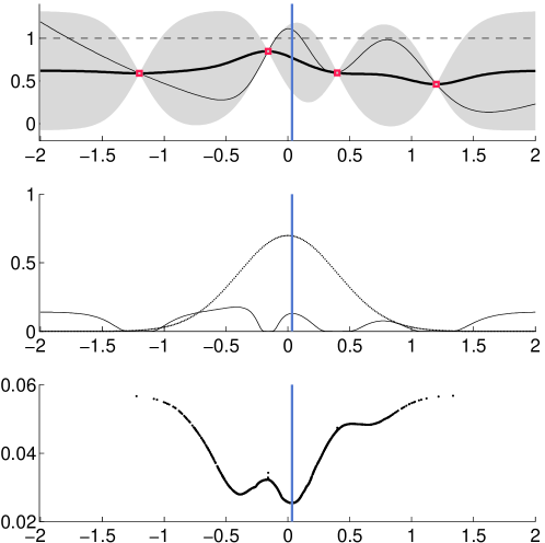
Figure 2: Illustration of a SUR strategy. This figure shows the initial design. Top: threshold $u=1$ (horizontal dashed line); function $f$ (thin line); $n=4$ initial evaluations (squares); kriging approximation $f_{n}$ (thick line); 95% confidence intervals computed from the kriging variance (shaded area). Middle: probability of excursion (solid line); probability density of $\mathsf{P}_{\mathds{X}}$ (dotted line). Bottom: graph of $J_{1,n=4}^{\text{\tiny SUR}}(Y_{i})$, $i=1,\ldots,m=1500$, the minimum of which indicates where the next evaluation of $f$ should be done (i.e., near the origin).

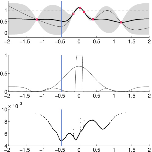
Figure 3: Illustration of a SUR strategy (see also Figures 2 and 4). This figure shows the progress of the SUR strategy after two iterations—a total of $n=6$ evaluations (squares) have been performed. The next evaluation point will be approximately at $x=-0.5$

.

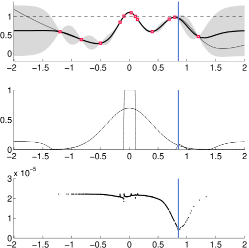
Figure 4: Illustration of a SUR strategy (see also Figures 2 and 3). This figure shows the progress of the SUR strategy after eight iterations—a total of $n=12$ evaluations (squares) have been performed. At this stage, the probability of excursion $p_{n}$ almost equals $0$ or $1$ in the region where the density of $\mathsf{P}_{\mathds{X}}$ is high.

5.2 An example in structural reliability

In this section, we evaluate all criteria discussed in Section 3 and Section 4 through a classical benchmark example in structural reliability (see, e.g., Borri and Speranzini, 1997; Waarts, 2000; Schueremans, 2001; Deheeger, 2008). Echard et al. (2010a, b) used this benchmark to make a comparison among several methods proposed in Schueremans and Gemert (2005), some of which are based on the construction of a response surface. The objective of the benchmark is to estimate the probability of failure of a so-called four-branch series system. A failure happens when the system is working under the threshold $u=0$. The performance function $f$ for this system is defined as

$$f:(x_{1},x_{2})\in\mathds{R}^{2}\mapsto f(x_{1},x_{2})=\min\left\{\begin{array}[]{ll}3+0.1(x_{1}-x_{2})^{2}-(x_{1}+x_{2})/\sqrt{2};\\ 3+0.1(x_{1}-x_{2})^{2}+(x_{1}+x_{2})/\sqrt{2};\\ (x_{1}-x_{2})+6/\sqrt{2};\\ (x_{2}-x_{1})+6/\sqrt{2}\end{array}\right\}\,.$$

The uncertain input factors are supposed to be independent and have standard normal distribution. Figure 5 shows the performance function, the failure domain and the input distribution. Observe that $f$ has a first-derivative discontinuity along four straight lines originating from the point $(0,0)$.

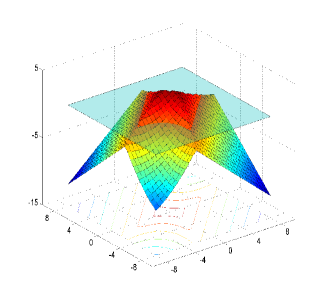
\psfrag{fff}{$f=0$}\includegraphics[width=170.71652pt,height=156.49014pt]{MCsample}

Figure 5: Left: mesh plot of the performance function $f$ corresponding to the four-branch series system; a failure happens when $f$ is below the transparent plane; Right: contour plot of $f$; limit state $f=0$ (thick line); sample of size $m=3\times 10^{3}$ from $\mathsf{P}_{\mathds{X}}$ (dots).

For each sequential method, we will follow the procedure described in Table 3. We generate an initial design of $n_{0}=10$ points (five times the dimension of the factor space) using a maximin LHS (Latin Hypercube Sampling) on $[-6;6]\times[-6;6]$. We choose a Monte Carlo sample of size $m=30000$. Since the true probability of failure is approximately $\alpha=0.4\%$ in this example, the coefficient of variation for $\alpha_{m}$ is $1/\sqrt{m\,\alpha}\approx 9\%$. The same initial design and Monte Carlo sample are used for all methods.

A Gaussian process with constant unknown mean and a Matérn covariance function is used as our prior information about $f$. The parameters of the Matérn covariance functions are estimated on the initial design by REML (see, e.g. Stein, 1999). In this experiment, we follow the common practice of re-estimating the parameters of the covariance function during the sequential strategy, but only once every ten iterations to save some computation time.

The probability of failure is estimated by (13). To evaluate the rate of convergence, we compute the number $n_{\gamma}$ of iterations that must be performed using a given strategy to observe a stabilization of the relative error of estimation within an interval of length $2\gamma$:

$$n_{\gamma}=\min\left\{n\geq 0;\forall k\geq n,\frac{\lvert\widehat{\alpha}_{n_{0}+k}-\alpha_{m}\rvert}{\alpha_{m}}<\gamma\right\}\,.$$

All the available sequential strategies are run 100 times, with different initial designs and Monte Carlo samples. The results for $\gamma=0.10$, $\gamma=0.03$ and $\gamma=0.01$ are summarized in Table 4. We shall consider that $n_{0.1}$ provides a measure of the performance of the strategy in the “initial phase”, where a rough estimate of $\alpha$ is to be found, whereas $n_{0.03}$ and $n_{0.01}$ measure the performance in the “refinement phase”.

The four variants of the SUR strategy (see Table 1) have been run with $Q=12$ and either $m_{0}=10$ or $m_{0}=500$. The performance are similar for all four variants and for both values of $m_{0}$. It appears, however, that the criterions $J_{1}^{\text{\tiny SUR}}$ and $J_{2}^{\text{\tiny SUR}}{2}$ (i.e., the criterions given directly by Proposition 3) are slightly better than $J_{3}^{\text{\tiny SUR}}$ and $J_{4}^{\text{\tiny SUR}}$; this will be confirmed by the simulations of Section 5.3. It also seems that the SUR algorithm is slightly slower to obtain a rough estimate of the probability of failure when $m_{0}$ is very small, but performs very well in the refinement phase. (Note that $m_{0}=10$ is a drastic pruning for a sample of size $m=30000$.)

The tIMSE strategy has been run for three different values of its tuning parameter $\sigma_{\varepsilon}^{2}$, using the pruning scheme with $m_{0}=500$. The best performance is obtained for $\sigma_{\varepsilon}^{2}\approx 0$, and is almost as good as the performance of SUR stragies with the same value of $m0$ (a small loss of performance, of about one evaluation on average, can be noticed in the refinement phase). Note that the required accuracy was not reached after 200 iterations in 17% of the runs for $\sigma_{\varepsilon}^{2}=1$. In fact, the tIMSE strategy tends to behave like a space-filling strategy in this case. Figure 6 shows the points that have been evaluated in three cases: the evaluations are less concentrated on the boundary between the safe and the failure region when $\sigma_{\varepsilon}^{2}=1$.

Finally, the results obtained for $J^{\text{\tiny RB}}$ and $J^{\text{\tiny EGL}}$ indicate that the corresponding strategies are clearly less efficient in the “initial phase” than strategies based on $J_{1}^{\text{\tiny SUR}}$ or $J_{2}^{\text{\tiny SUR}}$. For $\gamma=0.1$, the average loss with respect to $J_{1}^{\text{\tiny SUR}}$ is between approximately $0.9$ evaluations for the best case (criterion $J^{\text{\tiny RB}}$ with $\delta=2$, $\kappa=2$) and $3.9$ evaluations for the worst case. For $\gamma=0.03$, the loss is between $1.4$ evaluations (also for (criterion $J^{\text{\tiny RB}}$ with $\delta=2$, $\kappa=2$) and $3.5$ evaluations. This loss of efficiency can also be observed very clearly on the $90^{\text{th}}$ percentile in the inital phase. Criterion $J^{\text{\tiny RB}}$ seems to perform best with $\delta=2$ and $\kappa=2$ in this experiment, but this will not be confirmed by the simulations of Section 5.3. Tuning the parameters of this criterion for the estimation of a probability of failure does not seem to be an easy task.

Table 4: Comparison of the convergence to $\alpha_{m}$ in the benchmark example Section 5.2 for different sampling strategies. The first number (bold text) is the average value of $n_{\gamma}$ over 100 runs. The numbers between brackets indicate the $10^{\text{th}}$ and $90^{\text{th}}$ percentile.

criterion	parameters	$\gamma=0.10$	$\gamma=0.03$	$\gamma=0.01$
$J_{1}^{\text{\tiny SUR}}$	$m_{0}=500$	16.1 [10–22]	25.7 [17–35]	36.0 [26–48]
	$m_{0}=10$	19.4 [11–28]	28.1 [19–38]	35.4 [26–44]
$J_{2}^{\text{\tiny SUR}}$	$m_{0}=500$	16.4 [10–24]	25.7 [19–33]	35.5 [25–45]
	$m_{0}=10$	20.0 [11–30]	28.3 [20–39]	35.3 [26–44]
$J_{3}^{\text{\tiny SUR}}$	$m_{0}=500$	18.2 [10–27]	26.9 [18–37]	35.9 [27–46]
	$m_{0}=10$	20.1 [11–30]	28.0 [20–36]	35.2 [25–44]
$J_{4}^{\text{\tiny SUR}}$	$m_{0}=500$	17.2 [10–28]	26.5 [20–36]	35.2 [25–45]
	$m_{0}=10$	21.4 [13–30]	28.9 [20–38]	35.5 [27–44]
$J^{\text{\tiny tIMSE}}$	$\sigma_{\varepsilon}^{2}=10^{-6}$	16.6 [10–23]	26.5 [19–36]	37.3 [28–49]
	$\sigma_{\varepsilon}^{2}=0.1$	15.9 [10–22]	29.1 [19–43]	50.5 [30–79]
	$\sigma_{\varepsilon}^{2}=1$	21.7 [11–31]	52.4 [31–85]	79.5 [42–133](∗)
$J^{\text{\tiny EGL}}$	–	21.0 [11–31]	29.2 [21–39]	36.4 [28–44]
$J^{\text{\tiny RB}}$	$\delta=1$, $\kappa=0.5$	18.7 [10–27]	27.5 [20–35]	36.6 [27–44]
	$\delta=1$, $\kappa=2.0$	18.9 [11–28]	28.3 [21–35]	37.7 [30–45]
	$\delta=2$, $\kappa=0.5$	17.6 [10–24]	27.6 [20–34]	37.1 [29–45]
	$\delta=2$, $\kappa=2.0$	17.0 [10–21]	27.1 [20–34]	36.8 [29–44]

(*) The required accuracy was not reached after 200 iterations in 17% of the runs

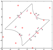
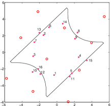
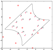
Figure 6: The first $16$ points (squares) evaluated using sampling criterion $J_{1}^{\text{\tiny SUR}}$ (left), $J^{\text{\tiny tIMSE}}$ with $\sigma_{\varepsilon}^{2}=0.1$ (middle), $J^{\text{\tiny tIMSE}}$ with $\sigma_{\varepsilon}^{2}=1$ (right). Numbers near squares indicate the order of evaluation. The location of the $n_{0}=10$ points of the initial design are indicated by circles.

5.3 Average performance on sample paths of a Gaussian process

This section provides a comparison of all the criteria introduced or recalled in this paper, on the basis of their average performance on the sample paths of a zero-mean Gaussian process defined on $\mathds{X}=\left[0,1\right]^{d}$, for $d\in\left\{1,2,3\right\}$. In all experiments, the same covariance function is used for the generation of the sample paths and for the computation of the sampling criteria. We have considered isotropic Matérn covariance functions, whose parameters are given in Table 5. An initial maximin LHS design of size $n_{0}$ (also given in the table) is used: note that the value of $n$ reported on the $x$-axis of Figures 8–11 is the total number of evaluations, including the initial design.

Table 5: Size of the initial design and covariance parameters for the experiments of Section 5.3. The parametrization of the Matérn covariance function used here is defined in Appendix A.

$d$	$n_{0}$	$\sigma^{2}$	$\nu$	$\rho$
$1$	$3$	$1.0$	$2.0$	$0.100$
$2$	$10$	$1.0$	$2.0$	$0.252$
$3$	$15$	$1.0$	$2.0$	$0.363$

The $d$ input variables are assumed to be independent and uniformly distributed on $[0,1]$, i.e., $\mathsf{P}_{\mathds{X}}$ is the uniform distribution on $\mathds{X}$. An $m$-sample $Y_{1}$, …, $Y_{m}$ from $\mathsf{P}_{\mathds{X}}$ is drawn one and for all, and used both for the approximation of integrals (in SUR and tIMSE criteria) and for the discrete search of the next sampling point (for all criteria). We take $m=500$ and use the same MC sample for all criteria in a given dimension $d$.

We adopt the meta-estimation framework as described in Section 3.3; in other words, our goal is to estimate the MC estimator $\alpha_{m}$. We choose to adjust the threshold $u$ in order to have $\alpha_{m}=0.02$ for all sample paths (note that, as a consequence, there are exactly $m\alpha_{m}=10$ points in the failure region) and we measure the performance of a strategy after $n$ evaluations by its relative mean-square error (MSE) expressed in decibels (dB):

$$\mathrm{rMSE}\;:=\;10\,\log_{10}\left(\;\frac{1}{L}\,\sum_{l=1}^{L}\frac{\left(\widehat{\alpha}^{(l)}_{m,n}-\alpha_{m}\right)^{2}}{\alpha^{2}_{m}}\;\right)\,,$$

where $\widehat{\alpha}^{(l)}_{m,n}=\frac{1}{m}\sum_{j=1}^{m}p^{(l)}_{n}(Y_{j})$ is the posterior mean of the MC estimator $\alpha_{m}$ after $n$ evaluations on the $l^{\text{th}}$ simulated sample path ($L=4000$).

We use a sequential maximin strategy as a reference in all of our experiments. This simple space-filling strategy is defined by $X_{n+1}=\operatorname*{argmax}_{j}\,\min_{1\leq i\leq n}\left|Y_{j}-X_{i}\right|$, where the argmax runs over all indices $j$ such that $Y_{j}\not\in\left\{X_{1},\ldots,X_{n}\right\}$. Note that this strategy does not depend on the choice of a Gaussian process model.

Our first experiment (Figure 8 ) provides a comparison of the four SUR strategies proposed in Section 3.2. It appears that all of them perform roughly the same when compared to the reference strategy. A closer look, however, reveals that the strategies $J_{1}^{\text{\tiny SUR}}$ and $J_{2}^{\text{\tiny SUR}}$ provided by Proposition 3 perform slightly better than the other two (noticeably so in the case $d=3$).

The performance of the tIMSE strategy is shown on Figure 8 for several value of its tuning parameter $\sigma_{\varepsilon}^{2}$ (other values, not shown here, have been tried as well). It is clear that the performance of this strategy improves when $\sigma_{\varepsilon}^{2}$ goes to zero, whatever the dimension.

The performance of the strategy based on $J_{\kappa,\delta}^{\text{\tiny RB}}$ is shown on Figure 10 for several values of its parameters. It appears that the criterion proposed by Bichon et al. (2008), which corresponds to $\delta=1$, performs better than the one proposed by Ranjan et al. (2008), which corresponds to $\delta=2$, for the same value of $\kappa$. Moreover, the value $\kappa=0.5$ has been found in our experiments to produce the best results.

Figure 10 illustrates that the loss of performance associated to the “pruning trick” introduced in Section 3.4 can be negligible if the size $m_{0}$ of the pruned MC sample is large enough (here, $m_{0}$ has been taken equal to $50$). In practice, the value of $m_{0}$ should be chosen small enough to keep the overhead of the sequential strategy reasonable—in other words, large values of $m_{0}$ should only be used for very complex computer codes.

Finally, a comparison involving the best strategy obtained in each category is presented on Figure 11. The best result is consistently obtained with the SUR strategy based on $J_{1,n}^{\text{\tiny SUR}}$. The tIMSE strategy with $\sigma_{\varepsilon}^{2}\approx 0$ provides results which are almost as good. Note that both strategies are one-step lookahead strategies based on the approximation of the risk by an integral criterion, which makes them rather expensive to compute. Simpler strategies based on the marginal distribution (criteria $J_{n}^{\text{\tiny RB}}$ and $J_{n}^{\text{\tiny EGL}}$) provide interesting alternatives for moderately expensive computer codes: their performances, although not as good as those of one-step lookahead criterions, are still much better than that of the reference space-filling strategy.

\psfragscanon\psfrag{s10}[b][b]{\color[rgb]{0,0,0}\begin{tabular}[]{c}rMSE (dB)\end{tabular}}\psfrag{s11}[t][t]{\color[rgb]{0,0,0}\begin{tabular}[]{c}n\end{tabular}}\psfrag{s12}[b][b]{\color[rgb]{0,0,0}\begin{tabular}[]{c}rMSE (dB)\end{tabular}}\psfrag{s13}[t][t]{\color[rgb]{0,0,0}\begin{tabular}[]{c}n\end{tabular}}\psfrag{s14}[b][b]{\color[rgb]{0,0,0}\begin{tabular}[]{c}rMSE (dB)\end{tabular}}\psfrag{s15}[t][t]{\color[rgb]{0,0,0}\begin{tabular}[]{c}n\end{tabular}}\psfrag{s17}[lt][lt]{\begin{minipage}{142.26378pt}\scriptsize\begin{tabular}[]{ll}$J_{1}^{\text{\tiny SUR}}$&black solid line\\ $J_{2}^{\text{\tiny SUR}}$&gray solid line\\ $J_{3}^{\text{\tiny SUR}}$&gray mixed line\\ $J_{4}^{\text{\tiny SUR}}$&black mixed line\\ ref.&black dashed line\end{tabular} \vspace{2ex}\\ \begin{tabular}[]{ll}Upper-left:&$d=1$\\ Upper-right:&$d=2$\\ Lower-left:&$d=3$\\ \end{tabular} \end{minipage}}\psfrag{x01}[t][t]{0}\psfrag{x02}[t][t]{0.5}\psfrag{x03}[t][t]{1}\psfrag{x04}[t][t]{20}\psfrag{x05}[t][t]{40}\psfrag{x06}[t][t]{60}\psfrag{x07}[t][t]{80}\psfrag{x08}[t][t]{100}\psfrag{x09}[t][t]{20}\psfrag{x10}[t][t]{40}\psfrag{x11}[t][t]{60}\psfrag{x12}[t][t]{80}\psfrag{x13}[t][t]{10}\psfrag{x14}[t][t]{20}\psfrag{x15}[t][t]{30}\psfrag{v01}[r][r]{0}\psfrag{v02}[r][r]{0.5}\psfrag{v03}[r][r]{1}\psfrag{v04}[r][r]{-25}\psfrag{v05}[r][r]{-20}\psfrag{v06}[r][r]{-15}\psfrag{v07}[r][r]{-10}\psfrag{v08}[r][r]{-5}\psfrag{v09}[r][r]{-30}\psfrag{v10}[r][r]{-20}\psfrag{v11}[r][r]{-10}\psfrag{v12}[r][r]{0}\psfrag{v13}[r][r]{-30}\psfrag{v14}[r][r]{-20}\psfrag{v15}[r][r]{-10}\psfrag{v16}[r][r]{0}\psfrag{v17}[r][r]{10}\includegraphics{ap-sur.eps}

Figure 7: Relative MSE performance of several SUR strategies.

\psfragscanon\psfrag{s10}[b][b]{\color[rgb]{0,0,0}\begin{tabular}[]{c}rMSE (dB)\end{tabular}}\psfrag{s11}[t][t]{\color[rgb]{0,0,0}\begin{tabular}[]{c}n\end{tabular}}\psfrag{s12}[b][b]{\color[rgb]{0,0,0}\begin{tabular}[]{c}rMSE (dB)\end{tabular}}\psfrag{s13}[t][t]{\color[rgb]{0,0,0}\begin{tabular}[]{c}n\end{tabular}}\psfrag{s14}[b][b]{\color[rgb]{0,0,0}\begin{tabular}[]{c}rMSE (dB)\end{tabular}}\psfrag{s15}[t][t]{\color[rgb]{0,0,0}\begin{tabular}[]{c}n\end{tabular}}\psfrag{s17}[lt][lt]{\begin{minipage}{142.26378pt}\scriptsize\begin{tabular}[]{ll}$\sigma_{\varepsilon}^{2}=10^{-6}$&black solid line\\ $\sigma_{\varepsilon}^{2}=0.1$&gray solid line\\ $\sigma_{\varepsilon}^{2}=1$&black mixed line\\ ref.&black dashed line\end{tabular} \vspace{2ex}\\ \begin{tabular}[]{ll}Upper-left:&$d=1$\\ Upper-right:&$d=2$\\ Lower-left:&$d=3$\\ \end{tabular} \end{minipage}}\psfrag{x01}[t][t]{0}\psfrag{x02}[t][t]{0.5}\psfrag{x03}[t][t]{1}\psfrag{x04}[t][t]{20}\psfrag{x05}[t][t]{40}\psfrag{x06}[t][t]{60}\psfrag{x07}[t][t]{80}\psfrag{x08}[t][t]{100}\psfrag{x09}[t][t]{20}\psfrag{x10}[t][t]{40}\psfrag{x11}[t][t]{60}\psfrag{x12}[t][t]{80}\psfrag{x13}[t][t]{10}\psfrag{x14}[t][t]{20}\psfrag{x15}[t][t]{30}\psfrag{v01}[r][r]{0}\psfrag{v02}[r][r]{0.5}\psfrag{v03}[r][r]{1}\psfrag{v04}[r][r]{-25}\psfrag{v05}[r][r]{-20}\psfrag{v06}[r][r]{-15}\psfrag{v07}[r][r]{-10}\psfrag{v08}[r][r]{-5}\psfrag{v09}[r][r]{-30}\psfrag{v10}[r][r]{-20}\psfrag{v11}[r][r]{-10}\psfrag{v12}[r][r]{0}\psfrag{v13}[r][r]{-30}\psfrag{v14}[r][r]{-20}\psfrag{v15}[r][r]{-10}\psfrag{v16}[r][r]{0}\psfrag{v17}[r][r]{10}\includegraphics{ap-tIMSE.eps}

Figure 8: Relative MSE performance of the tIMSE strategy for several values of its parameter.

\psfragscanon\psfrag{s10}[b][b]{\color[rgb]{0,0,0}\begin{tabular}[]{c}rMSE (dB)\end{tabular}}\psfrag{s11}[t][t]{\color[rgb]{0,0,0}\begin{tabular}[]{c}n\end{tabular}}\psfrag{s12}[b][b]{\color[rgb]{0,0,0}\begin{tabular}[]{c}rMSE (dB)\end{tabular}}\psfrag{s13}[t][t]{\color[rgb]{0,0,0}\begin{tabular}[]{c}n\end{tabular}}\psfrag{s14}[b][b]{\color[rgb]{0,0,0}\begin{tabular}[]{c}rMSE (dB)\end{tabular}}\psfrag{s15}[t][t]{\color[rgb]{0,0,0}\begin{tabular}[]{c}n\end{tabular}}\psfrag{s17}[lt][lt]{\begin{minipage}{142.26378pt}\scriptsize\begin{tabular}[]{lll}$\kappa=0.5$&$\delta=1$&black solid line\\ $\kappa=0.5$&$\delta=2$&gray solid line\\ $\kappa=2$&$\delta=1$&black mixed line\\ $\kappa=2$&$\delta=2$&gray mixed line\\ ref.&&black dashed line\end{tabular} \vspace{2ex}\\ \begin{tabular}[]{ll}Upper-left:&$d=1$\\ Upper-right:&$d=2$\\ Lower-left:&$d=3$\end{tabular} \end{minipage}}\psfrag{x01}[t][t]{0}\psfrag{x02}[t][t]{0.5}\psfrag{x03}[t][t]{1}\psfrag{x04}[t][t]{20}\psfrag{x05}[t][t]{40}\psfrag{x06}[t][t]{60}\psfrag{x07}[t][t]{80}\psfrag{x08}[t][t]{100}\psfrag{x09}[t][t]{20}\psfrag{x10}[t][t]{40}\psfrag{x11}[t][t]{60}\psfrag{x12}[t][t]{80}\psfrag{x13}[t][t]{10}\psfrag{x14}[t][t]{20}\psfrag{x15}[t][t]{30}\psfrag{v01}[r][r]{0}\psfrag{v02}[r][r]{0.5}\psfrag{v03}[r][r]{1}\psfrag{v04}[r][r]{-25}\psfrag{v05}[r][r]{-20}\psfrag{v06}[r][r]{-15}\psfrag{v07}[r][r]{-10}\psfrag{v08}[r][r]{-5}\psfrag{v09}[r][r]{-30}\psfrag{v10}[r][r]{-20}\psfrag{v11}[r][r]{-10}\psfrag{v12}[r][r]{0}\psfrag{v13}[r][r]{-30}\psfrag{v14}[r][r]{-20}\psfrag{v15}[r][r]{-10}\psfrag{v16}[r][r]{0}\psfrag{v17}[r][r]{10}\includegraphics{ap-rb.eps}

Figure 9: Relative MSE performance of the $J^{\text{\tiny RB}}$ criterion, for several values of its parameters.

\psfragscanon\psfrag{s10}[b][b]{\color[rgb]{0,0,0}\begin{tabular}[]{c}rMSE (dB)\end{tabular}}\psfrag{s11}[t][t]{\color[rgb]{0,0,0}\begin{tabular}[]{c}n\end{tabular}}\psfrag{s12}[b][b]{\color[rgb]{0,0,0}\begin{tabular}[]{c}rMSE (dB)\end{tabular}}\psfrag{s13}[t][t]{\color[rgb]{0,0,0}\begin{tabular}[]{c}n\end{tabular}}\psfrag{s14}[b][b]{\color[rgb]{0,0,0}\begin{tabular}[]{c}rMSE (dB)\end{tabular}}\psfrag{s15}[t][t]{\color[rgb]{0,0,0}\begin{tabular}[]{c}n\end{tabular}}\psfrag{s17}[lt][lt]{\begin{minipage}{142.26378pt}\scriptsize\begin{tabular}[]{ll}$J_{1}^{\text{\tiny SUR}}$&full line\\ $J_{3}^{\text{\tiny SUR}}$&mixed line\\ without pruning&black\\ pruning $m_{0}=50$&gray\\ ref.&black dashed line\end{tabular} \vspace{2ex}\\ \begin{tabular}[]{ll}Upper-left:&$d=1$\\ Upper-right:&$d=2$\\ Lower-left:&$d=3$\\ \end{tabular} \end{minipage}}\psfrag{x01}[t][t]{0}\psfrag{x02}[t][t]{0.5}\psfrag{x03}[t][t]{1}\psfrag{x04}[t][t]{20}\psfrag{x05}[t][t]{40}\psfrag{x06}[t][t]{60}\psfrag{x07}[t][t]{80}\psfrag{x08}[t][t]{100}\psfrag{x09}[t][t]{20}\psfrag{x10}[t][t]{40}\psfrag{x11}[t][t]{60}\psfrag{x12}[t][t]{80}\psfrag{x13}[t][t]{10}\psfrag{x14}[t][t]{20}\psfrag{x15}[t][t]{30}\psfrag{v01}[r][r]{0}\psfrag{v02}[r][r]{0.5}\psfrag{v03}[r][r]{1}\psfrag{v04}[r][r]{-25}\psfrag{v05}[r][r]{-20}\psfrag{v06}[r][r]{-15}\psfrag{v07}[r][r]{-10}\psfrag{v08}[r][r]{-5}\psfrag{v09}[r][r]{-30}\psfrag{v10}[r][r]{-20}\psfrag{v11}[r][r]{-10}\psfrag{v12}[r][r]{0}\psfrag{v13}[r][r]{-40}\psfrag{v14}[r][r]{-20}\psfrag{v15}[r][r]{0}\includegraphics{ap-m0.eps}

Figure 10: Relative MSE performance of two SUR criteria, with and without the “pruning trick” described in Section 3.4. The black and gray lines are almost surimposed for each of the criterions $J_{1}^{\text{\tiny SUR}}$ and $J_{3}^{\text{\tiny SUR}}$.

\psfragscanon\psfrag{s10}[b][b]{\color[rgb]{0,0,0}\begin{tabular}[]{c}rMSE (dB)\end{tabular}}\psfrag{s11}[t][t]{\color[rgb]{0,0,0}\begin{tabular}[]{c}n\end{tabular}}\psfrag{s12}[b][b]{\color[rgb]{0,0,0}\begin{tabular}[]{c}rMSE (dB)\end{tabular}}\psfrag{s13}[t][t]{\color[rgb]{0,0,0}\begin{tabular}[]{c}n\end{tabular}}\psfrag{s14}[b][b]{\color[rgb]{0,0,0}\begin{tabular}[]{c}rMSE (dB)\end{tabular}}\psfrag{s15}[t][t]{\color[rgb]{0,0,0}\begin{tabular}[]{c}n\end{tabular}}\psfrag{s17}[lt][lt]{\begin{minipage}{142.26378pt}\scriptsize\begin{tabular}[]{ll}$J_{1}^{\text{\tiny SUR}}$&black solid line\\ tIMSE ($\sigma_{\varepsilon}^{2}=10^{-6}$)&gray solid line\\ $J^{\text{\tiny RB}}$ ($\kappa=0.5$, $\delta=1$)&black mixed line\\ $J^{\text{\tiny EGL}}$&gray mixed line\\ ref.&black dashed line\\ \end{tabular} \vspace{2ex}\\ \begin{tabular}[]{ll}Upper-left:&$d=1$\\ Upper-right:&$d=2$\\ Lower-left:&$d=3$\\ \end{tabular} \end{minipage}}\psfrag{x01}[t][t]{0}\psfrag{x02}[t][t]{0.5}\psfrag{x03}[t][t]{1}\psfrag{x04}[t][t]{20}\psfrag{x05}[t][t]{40}\psfrag{x06}[t][t]{60}\psfrag{x07}[t][t]{80}\psfrag{x08}[t][t]{100}\psfrag{x09}[t][t]{20}\psfrag{x10}[t][t]{40}\psfrag{x11}[t][t]{60}\psfrag{x12}[t][t]{80}\psfrag{x13}[t][t]{10}\psfrag{x14}[t][t]{20}\psfrag{x15}[t][t]{30}\psfrag{v01}[r][r]{0}\psfrag{v02}[r][r]{0.5}\psfrag{v03}[r][r]{1}\psfrag{v04}[r][r]{-25}\psfrag{v05}[r][r]{-20}\psfrag{v06}[r][r]{-15}\psfrag{v07}[r][r]{-10}\psfrag{v08}[r][r]{-5}\psfrag{v09}[r][r]{-30}\psfrag{v10}[r][r]{-20}\psfrag{v11}[r][r]{-10}\psfrag{v12}[r][r]{0}\psfrag{v13}[r][r]{-30}\psfrag{v14}[r][r]{-20}\psfrag{v15}[r][r]{-10}\psfrag{v16}[r][r]{0}\psfrag{v17}[r][r]{10}\includegraphics{ap-all.eps}

Figure 11: Relative MSE performance the best strategy in each category.

6 Concluding remarks

One of the main objectives of this paper was to present a synthetic viewpoint on sequential strategies based on a Gaussian process model and kriging for the estimation of a probability of failure. The starting point of this presentation is a Bayesian decision-theoretic framework from which the theoretical form of an optimal strategy for the estimation of a probability of failure can be derived. Unfortunately, the dynamic programming problem corresponding to this strategy is not numerically tractable. It is nonetheless possible to derive from there the ingredients of a sub-optimal strategy: the idea is to focus on one-step lookahead suboptimal strategies, where the exact risk is replaced by a substitute risk that accounts for the information gain about $\alpha$ expected from a new evaluation. We call such a strategy a stepwise uncertainty reduction (SUR) strategy. Our numerical experiments show that SUR strategies perform better, on average, than the other strategies proposed in the literature. However, this comes at a higher computational cost than strategies based only on marginal distributions. The tIMSE sampling criterion, which seems to have a convergence rate comparable to that of the SUR criterions when $\sigma_{\varepsilon}^{2}\approx 0$, also has a high computational complexity.

In which situations can we say that the sequential strategies presented in this paper are interesting alternatives to classical importance sampling methods for estimating a probability of failure, for instance the subset sampling method of Au and Beck (2001)? In our opinion, beyond the obvious role of the simulation budget $N$, the answer to this question depends on our capacity to elicit an appropriate prior. In the example of Section 5.2, as well as in many other examples of the literature using Gaussian processes in the domain of computer experiments, the prior is easy to choose because $\mathds{X}$ is a low-dimensional space and $f$ tends to be smooth. Then, the plug-in approach which consists in using ML or REML to estimate the parameters of the covariance function of the Gaussian process after each new evaluation is likely to succeed. If $\mathds{X}$ is high-dimensional and $f$ is expensive to evaluate, difficulties arise. In particular, our sampling strategies do not take into account our uncertain knowledge of the covariance parameters, and there is no guarantee that ML estimation will do well when the points are chosen by a sampling strategy that favors some localized target region (the neighboorhood the frontier of the domain of failure in this paper, but the question is equally relevant in the field optimization, for instance). The difficult problem of deciding the size $n_{0}$ of the initial design is crucial in this connection. Fully Bayes procedures constitute a possible direction for future research, as long as they don’t introduce an unacceptable computational overhead. Whatever the route, we feel that the robustness of Gaussian process-based sampling strategies with respect to the procedure of estimation of the covariance parameters should be addressed carefully in order to make these methods usable in the industrial world.

Software. We would like to draw the reader’s attention on the recently published package KrigInv (Picheny and Ginsbourger, 2011) for the statistical computing environment R (see Hornik, 2010). This package provides an open source (GPLv3) implementation of all the strategies proposed in this paper. Please note that the simulation results presented in this paper were not obtained using this package, that was not available at the time of its writing.

Appendix

Appendix A The Matérn covariance

The exponential covariance and the Matérn covariance are among the most conventionally used stationary covariances in the literature of design and analysis of computer experiments. The Matérn covariance class (Yaglom, 1986) offers the possibility to adjust the regularity of $\xi$ with a single parameter. Stein (1999) advocates the use of the following parametrization of the Matérn function:

$$\kappa_{\nu}(h)=\frac{1}{2^{\nu-1}\Gamma(\nu)}\left(2\nu^{1/2}h\right)^{\nu}\mathcal{K}_{\nu}\left(2\nu^{1/2}h\right)\,,\quad h\in\mathds{R}$$ (35)

where $\Gamma$ is the Gamma function and $\mathcal{K}_{\nu}$ is the modified Bessel function of the second kind. The parameter $\nu>0$ controls regularity at the origin of the function. To model a real-valued function $f$ defined over $\mathds{X}\subset\mathds{R}^{d}$, with $d\geq 1$, we use the following anisotropic form of the Matérn covariance:

$$k_{\theta}(x,y)=\sigma^{2}\kappa_{\nu}\left(\sqrt{\sum_{i=1}^{d}\frac{(x_{[i]}-y_{[i]})^{2}}{\rho_{i}^{2}}}\right)\,,\quad x,y\in\mathds{R}^{d}$$ (36)

where $x_{[i]},y_{[i]}$ denote the $i^{\rm th}$ coordinate of $x$ and $y$, the positive scalar $\sigma^{2}$ is a variance parameter (we have $k_{\theta}(x,x)=\sigma^{2}$), and the positive scalars $\rho_{i}$ represent scale or range parameters of the covariance, i.e., characteristic correlation lengths. Since $\sigma^{2}>0,\nu>0,\rho_{i}>0$, $i=1,\ldots,d$, we can take the logarithm of these scalars, and consider the vector of parameters $\theta=\{\log\sigma^{2},\log\nu,-\log\rho_{1},\ldots,-\log\rho_{d}\}\in\mathds{R}^{d+2}$, which is a practical parameterization when $\sigma^{2},\nu,\rho_{i}$, $i=1,\ldots,d$, need to be estimated from data.

Appendix B Proof of Proposition 4

a) Using the identity $\Phi^{-1}(1-p)=-\,\Phi^{-1}(p)$, we get

$$\bigl{|}U+\Phi^{-1}(1-p)\bigr{|}\;=\;\left|U-\Phi^{-1}(p)\right|\;\stackrel{{\scriptstyle\mbox{\scriptsize d}}}{{=}}\;\left|U+\Phi^{-1}(p)\right|,$$

where $\stackrel{{\scriptstyle\mbox{\scriptsize d}}}{{=}}$ denotes an equality in distribution. Therefore $G_{\kappa,\delta}(1-p)=G_{\kappa,\delta}(p)$.

b) Let $S_{p}=\max\bigl{(}0,\kappa^{\delta}-\bigl{|}\Phi^{-1}(p)+U\bigr{|}\bigr{)}$. Straightforward computations show that $t\mapsto\mathsf{P}\left(\left|t+U\right|\leq v\right)$ is strictly decreasing to $0$ on $\left[0,+\infty\right[$, for all $v>0$. As a consequence, $p\mapsto\mathsf{P}\bigl{(}S_{p}<s\bigr{)}$ is strictly increasing to $1$ on $\left[1/2,1\right[$, for all $s\in\bigl{]}0,\kappa^{\delta}\bigr{[}$. Therefore, $G_{\kappa,\delta}$ is strictly decreasing on $\left[1/2,1\right[$ and tends to zeros when $p\to 1$. The other assertions then follow from a).

c) Recall that $\xi(x)\sim\mathcal{N}\bigl{(}\widehat{\xi}_{n}(x),\sigma_{n}^{2}(x)\bigr{)}$ under $\mathsf{P}_{n}$. Therefore $U:=\bigl{(}\xi(x)-\widehat{\xi}_{n}(x)\bigr{)}/\sigma_{n}(x)\sim\mathcal{N}(0,1)$ under $\mathsf{P}_{n}$, and the result follows by substitution in (31).

The closed-form expressions of Ranjan et al.’s and Bichon and al.’s criteria (assertions d) and e)) is established in the following sections.

B.1 A preliminary decomposition common to both criteria

Recall that $t=\Phi^{-1}(1-p)$, $t^{+}=t+\kappa$ and $t^{-}=t-\kappa$. Then,

$$G_{\kappa,\delta}(p)\;=\; \ G_{\kappa,\delta}(1-p)\;=\;\mathsf{E}\left(\max\Bigl{(}0,\kappa^{\delta}-\bigl{|}t-U\bigr{|}^{\delta}\Bigr{)}\right)$$

$$\;=\; \ \int_{\kappa^{\delta}-\left|t-u\right|^{\delta}\geq 0}\left(\kappa^{\delta}-\left|t-u\right|^{\delta}\right)\,\varphi(u)\,\mathrm{d}u$$

$$\;=\; \ \int_{t^{-}}^{t^{+}}\left(\kappa^{\delta}-\left|t-u\right|^{\delta}\right)\,\varphi(u)\,\mathrm{d}u$$

$$\;=\; \ \kappa^{\delta}\left(\Phi(t^{+})-\Phi(t^{-})\right)\,-\,\underbrace{\int_{t^{-}}^{t^{+}}\left|t-u\right|^{\delta}\varphi(u)\,\mathrm{d}u}_{\text{Term $A$}}.$$ (37)

The computation of the integral $A$ will be carried separately in the next two sections for $\delta=1$ and $\delta=2$. For this purpose, we shall need the following elementary results:

$$\int_{a}^{b}u\varphi(u)\mathrm{d}u\;=\; \varphi(a)-\varphi(b)\,,$$ (38)

$$\int_{a}^{b}u^{2}\varphi(u)\mathrm{d}u\;=\; a\varphi(a)-b\varphi(b)+\Phi(b)-\Phi(a)\,.$$ (39)

B.2 Case $\delta=1$

Let us compute the value $A_{1}$ of the integral $A$ for $\delta=1$:

$$A_{1}\;=\; \int_{t^{-}}^{t^{+}}\left|t-u\right|\varphi(u)\mathrm{d}u\;=\;\int_{t^{-}}^{t}(t-u)\varphi(u)\mathrm{d}u+\int_{t}^{t^{+}}(u-t)\varphi(u)\mathrm{d}u$$

$$\;=\; t\left(\int_{t^{-}}^{t}\varphi(u)\,\mathrm{d}u-\int_{t}^{t^{+}}\varphi(u)\,\mathrm{d}u\right)-\int_{t^{-}}^{t}u\varphi(u)\,\mathrm{d}u+\int_{t}^{t^{+}}u\varphi(u)\,\mathrm{d}u$$

$$\;=\; t\left(2\Phi(t)-\Phi(t^{-})-\Phi(t^{+})\right)\,+\,2\varphi(t)-\varphi(t^{-})-\varphi(t^{+})\,,$$ (40)

where (38) has been used to get the final result. Plugging (40) into (37) yields (33).

B.3 Case $\delta=2$

Let us compute the value $A_{2}$ of the integral $A$ for $\delta=2$:

$$A_{2}\;=\; \int_{t^{-}}^{t^{+}}(t-u)^{2}\varphi(u)\,\mathrm{d}u$$

$$\;=\; t^{2}\int_{t^{-}}^{t^{+}}\varphi(u)\,\mathrm{d}u-2t\int_{t^{-}}^{t^{+}}u\varphi(u)\,\mathrm{d}u+\int_{t^{-}}^{t^{+}}u^{2}\varphi(u)\,\mathrm{d}u$$

$$\;=\; t^{2}\left(\Phi(t^{+})-\Phi(t^{-})\right)\,-\,2t\left(\varphi(t^{-})-\varphi(t^{+})\right)$$

$$+\,t^{-}\varphi(t^{-})-t^{+}\varphi(t^{+})\,+\,\Phi(t^{+})-\Phi(t^{-})\,,$$ (41)

where (38) and (39) have been used to get the final result. Plugging (40) into (37) yields (34).

References

- Arnaud et al. (2010) Arnaud, A., Bect, J., Couplet, M., Pasanisi, A., Vazquez, E.: Évaluation d’un risque d’inondation fluviale par planification séquentielle d’expériences. In: 42èmes Journées de Statistique (2010)
- Au and Beck (2001) Au, S.K., Beck, J.: Estimation of small failure probabilities in high dimensions by subset simulation. Probab. Engrg. Mechan. 16(4), 263–277 (2001)
- Bayarri et al. (2007) Bayarri, M.J., Berger, J.O., Paulo, R., Sacks, J., Cafeo, J.A., Cavendish, J., Lin, C.H., Tu, J.: A framework for validation of computer models. Technometrics 49(2), 138–154 (2007)
- Berry and Fristedt (1985) Berry, D.A., Fristedt, B.: Bandit problems: sequential allocation of experiments. Chapman & Hall (1985)
- Bertsekas (1995) Bertsekas, D.P.: Dynamic programming and optimal control vol. 1. Athena Scientific (1995)
- Bichon et al. (2008) Bichon, B.J., Eldred, M.S., Swiler, L.P., Mahadevan, S., McFarland, J.M.: Efficient global reliability analysis for nonlinear implicit performance functions. AIAA Journal 46(10), 2459–2468 (2008)
- Bjerager (1990) Bjerager, P.: On computational methods for structural reliability analysis. Structural Safety 9, 76–96 (1990)
- Borri and Speranzini (1997) Borri, A., Speranzini, E.: Structural reliability analysis using a standard deterministic finite element code. Structural Safety 19(4), 361–382 (1997)
- Box and Draper (1987) Box, G.E.P., Draper, N.R.: Empirical Model-Building and Response Surfaces. Wiley (1987)
- Bucher and Bourgund (1990) Bucher, C.G., Bourgund, U.: A fast and efficient response surface approach for structural reliability problems. Structural Safety 7(1), 57–66 (1990)
- Chilès and Delfiner (1999) Chilès, J.P., Delfiner, P.: Geostatistics: Modeling Spatial Uncertainty. Wiley, New York (1999)
- Currin et al. (1991) Currin, C., Mitchell, T., Morris, M., Ylvisaker, D.: Bayesian prediction of deterministic functions, with applications to the design and analysis of computer experiments. J. Amer. Statist. Assoc. 86(416), 953–963 (1991)
- Deheeger (2008) Deheeger, F.: Couplage mécano-fiabiliste : 2SMART – méthodologie d’apprentissage stochastique en fiabilité. Ph.D. thesis, Université Blaise Pascal – Clermont II (2008)
- Deheeger and Lemaire (2007) Deheeger, F., Lemaire, M.: Support vector machine for efficient subset simulations: 2SMART method. In: Kanda, J., Takada, T., Furuta, H. (eds.) 10th International Conference on Application of Statistics and Probability in Civil Engineering, Proceedings and Monographs in Engineering, Water and Earth Sciences, pp. 259–260. Taylor & Francis (2007)
- Echard et al. (2010a) Echard, B., Gayton, N., Lemaire, M.: Kriging-based Monte Carlo simulation to compute the probability of failure efficiently: AK-MCS method. In: 6èmes Journées Nationales de Fiabilité, 24–26 mars, Toulouse, France (2010a)
- Echard et al. (2010b) Echard, B., Gayton, N., Lemaire, M.: Structural reliability assessment using kriging metamodel and active learning. In: IFIP WG 7.5 Working Conference on Reliability and Optimization of Structural Systems (2010b)
- Fleuret and Geman (1999) Fleuret, F., Geman, D.: Graded learning for object detection. In: Proceedings of the workshop on Statistical and Computational Theories of Vision of the IEEE International Conference on Computer Vision and Pattern Recognition (CVPR/SCTV) (1999)
- Frazier et al. (2008) Frazier, P.I., Powell, W.B., Dayanik, S.: A knowledge-gradient policy for sequential information collection. SIAM Journal on Control and Optimization 47(5), 2410–2439 (2008)
- Ginsbourger (2009) Ginsbourger, D.: Métamodèles multiples pour l’approximation et l’optimisation de fonctions numériques multivariables. Ph.D. thesis, Ecole nationale supérieure des Mines de Saint-Etienne (2009)
- Ginsbourger et al. (2010) Ginsbourger, D., Le Riche, R., L., C.: Kriging is well-suited to parallelize optimization. In: Hiot, L.M., Ong, Y.S., Tenne, Y., Goh, C.K. (eds.) Computational Intelligence in Expensive Optimization Problems, Adaptation Learning and Optimization, vol. 2, pp. 131–162. Springer (2010)
- Handcock and Stein (1993) Handcock, M.S., Stein, M.L.: A bayesian analysis of kriging. Technometrics 35(4), 403–410 (1993)
- Hornik (2010) Hornik, K.: The R FAQ (2010). URL http://CRAN.R-project.org/doc/FAQ/R-FAQ.html. ISBN 3-900051-08-9
- Hurtado (2004) Hurtado, J.E.: An examination of methods for approximating implicit limit state functions from the viewpoint of statistical learning theory. Structural Safety 26(3), 271–293 (2004)
- Hurtado (2007) Hurtado, J.E.: Filtered importance sampling with support vector margin: A powerful method for structural reliability analysis. Structural Safety 29(1), 2–15 (2007)
- Jones et al. (1998) Jones, D.R., Schonlau, M., William, J.: Efficient global optimization of expensive black-box functions. Journal of Global Optimization 13(4), 455–492 (1998)
- Kennedy and O’Hagan (2001) Kennedy, M., O’Hagan, A.: Bayesian calibration of computer models. Journal of the Royal Statistical Society. Series B (Statistical Methodology) 63(3), 425–464 (2001)
- Kimeldorf and Wahba (1970) Kimeldorf, G.S., Wahba, G.: A correspondence between Bayesian estimation on stochastic processes and smoothing by splines. Ann. Math. Statist. 41(2), 495–502 (1970)
- Kushner (1964) Kushner, H.J.: A new method of locating the maximum point of an arbitrary multipeak curve in the presence of noise. J. Basic Engineering 86, 97–106 (1964)
- Loeppky et al. (2009) Loeppky, J.L., Sacks, J., Welch, W.J.: Choosing the sample size of a computer experiment: A practical guide. Technometrics 51(4), 366–376 (2009)
- Mockus (1989) Mockus, J.: Bayesian Approach to Global Optimization. Theory and Applications. Kluwer Academic Publisher, Dordrecht (1989)
- Mockus et al. (1978) Mockus, J., Tiesis, V., Zilinskas, A.: The application of Bayesian methods for seeking the extremum. In: Dixon, L., Szego, E.G. (eds.) Towards Global Optimization, vol. 2, pp. 117–129. Elsevier (1978)
- Oakley (2004) Oakley, J.: Estimating percentiles of uncertain computer code outputs. J. Roy. Statist. Soc. Ser. C 53(1), 83–93 (2004)
- Oakley and O’Hagan (2002) Oakley, J., O’Hagan, A.: Bayesian inference for the uncertainty distribution of computer model outputs. Biometrika 89(4) (2002)
- Oakley and O’Hagan (2004) Oakley, J., O’Hagan, A.: Probabilistic sensitivity analysis of complex models: a Bayesian approach. Journal of the Royal Statistical Society: Series B (Statistical Methodology) 66(3), 751–769 (2004)
- O’Hagan (1978) O’Hagan, A.: Curve fitting and optimal design for prediction. Journal of the Royal Statistical Society. Series B (Methodological) 40(1), 1–42 (1978)
- Parzen (1962) Parzen, E.: An approach to time series analysis. Ann. Math. Stat. 32, 951–989 (1962)
- Paulo (2005) Paulo, R.: Default priors for gaussian processes. Annals of Statistics 33(2), 556–582 (2005)
- Picheny and Ginsbourger (2011) Picheny, V., Ginsbourger, D.: KrigInv : Kriging-based inversion for deterministic and noisy computer experiments, version 1.1 (2011). URL http://cran.r-project.org/web/packages/KrigInv
- Picheny et al. (2010) Picheny, V., Ginsbourger, D., Roustant, O., Haftka, R.T., Kim, N.H.: Adaptive designs of experiments for accurate approximation of target regions (2010)
- Piera-Martinez (2008) Piera-Martinez, M.: Modélisation des comportements extrêmes en ingénierie. Ph.D. thesis, Université Paris Sud - Paris XI (2008)
- Pradlwarter et al. (2007) Pradlwarter, H., Schuëller, G., Koutsourelakis, P., Charmpis, D.: Application of line sampling simulation method to reliability benchmark problems. Structural Safety 29(3), 208 – 221 (2007). A Benchmark Study on Reliability in High Dimensions
- Press et al. (1992) Press, W.H., Teukolsky, S.A., Vetterling, W.T., Flannery, B.P.: Numerical Recipes in C. The Art of Scientific Computing (Second Edition). Cambridge University Press (1992)
- Rajashekhar and Ellingwood (1993) Rajashekhar, M.R., Ellingwood, B.R.: A new look at the response surface approach for reliability analysis. Structural Safety 12(3), 205–220 (1993)
- Ranjan et al. (2008) Ranjan, P., Bingham, D., Michailidis, G.: Sequential experiment design for contour estimation from complex computer codes. Technometrics 50(4), 527–541 (2008)
- Rubinstein and Kroese (2004) Rubinstein, R., Kroese, D.: The Cross-Entropy Method. Springer (2004)
- Sacks et al. (1989) Sacks, J., Welch, W.J., Mitchell, T.J., Wynn, H.P.: Design and analysis of computer experiments. Statistical Science 4(4), 409–435 (1989)
- Santner et al. (2003) Santner, T.J., Williams, B.J., Notz, W.: The Design and Analysis of Computer Experiments. Springer Verlag (2003)
- Schueremans (2001) Schueremans, L.: Probabilistic evaluation of structural unreinforced masonry. Ph.D. thesis, Catholic University of Leuven (2001)
- Schueremans and Gemert (2005) Schueremans, L., Gemert, D.V.: Benefit of splines and neural networks in simulation based structural reliability analysis. Structural safety 27(3), 246–261 (2005)
- Stein (1999) Stein, M.L.: Interpolation of Spatial Data: Some Theory for Kriging. Springer, New York (1999)
- Vazquez and Bect (2009) Vazquez, E., Bect, J.: A sequential Bayesian algorithm to estimate a probability of failure. In: Proceedings of the 15th IFAC Symposium on System Identification, SYSID 2009 15th IFAC Symposium on System Identification, SYSID 2009. Saint-Malo France (2009)
- Vazquez and Piera-Martinez (2007) Vazquez, E., Piera-Martinez, M.: Estimation du volume des ensembles d’excursion d’un processus gaussien par krigeage intrinsèque. In: 39ème Journées de Statistiques Conférence Journée de Statistiques. Angers France (2007)
- Vestrup (2003) Vestrup, E.M.: The Theory of Measures and Integration. Wiley (2003)
- Villemonteix (2008) Villemonteix, J.: Optimisation de fonctions coûteuses. Ph.D. thesis, Université Paris-Sud XI, Faculté des Sciences d’Orsay (2008)
- Villemonteix et al. (2009) Villemonteix, J., Vazquez, E., Walter, E.: An informational approach to the global optimization of expensive-to-evaluate functions. Journal of Global Optimization 44(4), 509–534 (2009)
- Waarts (2000) Waarts, P.H.: Structural reliability using finite element methods: an appraisal of DARS. Ph.D. thesis, Delft University of Technology (2000)
- Welch et al. (1992) Welch, W.J., Buck, R.J., Sacks, J., Wynn, H.P., Mitchell, T.J., Morris, M.D.: Screening, predicting and computer experiments. Technometrics 34, 15–25 (1992)
- Yaglom (1986) Yaglom, A.M.: Correlation Theory of Stationary and Related Random Functions I: Basic Results. Springer Series in Statistics. Springer-Verlag, New york (1986)