Low rank multivariate regression

Abstract.

We consider in this paper the multivariate regression problem, when the target regression matrix $A$ is close to a low rank matrix. Our primary interest is in on the practical case where the variance of the noise is unknown. Our main contribution is to propose in this setting a criterion to select among a family of low rank estimators and prove a non-asymptotic oracle inequality for the resulting estimator. We also investigate the easier case where the variance of the noise is known and outline that the penalties appearing in our criterions are minimal (in some sense). These penalties involve the expected value of Ky-Fan norms of some random matrices. These quantities can be evaluated easily in practice and upper-bounds can be derived from recent results in random matrix theory.

1. Introduction

We build on ideas introduced in a recent paper of Bunea, She and Wegkamp [7, 8] for the multivariate regression problem

(1) $$Y=XA+\sigma E$$

where $Y$ is a $m\times n$ matrix of response variables, $X$ is a $m\times p$ matrix of predictors, $A$ is $p\times n$ matrix of regression coefficients and $E$ is a $m\times n$ random matrix with i.i.d. entries. We assume for simplicity that the entries $E_{i,j}$ are standard Gaussian, yet all the results can be extended to the case where the entries are sub-Gaussian.

An important issue in multivariate regression is to estimate $A$ or $XA$ when the matrix $A$ has a low rank or can be well approximated by a low rank matrix, see Izenman [14]. In this case, a small number of linear combinations of the predictors catches most of the non-random variation of the response $Y$. This framework arises in many applications, among which analysis of fMRI image data [11], analysis of EEG data decoding [2], neural response modeling [6] or genomic data analysis [7].

When the variance $\sigma^{2}$ is known, the strategy developed by Bunea et al. [7] for estimating $A$ or $XA$ is the following. Writing $\|.\|$ for the Hilbert-Schmidt norm and $\widehat{A}_{r}$ for the minimizer of $\|Y-X\widehat{A}\|$ over the matrices $\widehat{A}$ of rank at most $r$, the matrix $XA$ is estimated by $X\widehat{A}_{\hat{r}}$, where $\hat{r}$ minimizes the criterion

(2) $${\mathrm{Crit}}_{\sigma^{2}}(r)=\|Y-X\widehat{A}_{r}\|^{2}+{\mathrm{pen}}_{\sigma^{2}}(r)\sigma^{2}.$$

Bunea et al. [7] considers a penalty ${\mathrm{pen}}_{\sigma^{2}}(r)$ linear in $r$ and provides clean non-asymptotic bounds on $\|X\widehat{A}_{\hat{r}}-XA\|^{2}$, on $\|\widehat{A}_{\hat{r}}-A\|^{2}$ and on the probability that the estimated rank $\hat{r}$ coincides with the rank of $A$.

Our main contribution is to propose and analyze a criterion to handle the case where $\sigma^{2}$ is unknown. Our theory requires no assumption on the design matrix $X$ and applies in particular when the sample size $m$ is smaller than the number of covariates $p$. We also exhibit a minimal sublinear penalty for the Criterion (2) for the case of known variance.

Let us denote by $q$ the rank of $X$ and by $G_{q\times n}$ a $q\times n$ random matrix with i.i.d. standard Gaussian entries. The penalties that we introduce involve the expected value of the Ky-Fan $(2,r)$-norm of the random matrix $G_{q\times n}$, namely

$$\mathcal{S}_{q\times n}(r)={\mathbb{E}}\left[{\|G_{q\times n}\|_{(2,r)}}\right],\quad\textrm{where}\;\ \|G_{q\times n}\|_{(2,r)}^{2}=\sum_{k=1}^{r}\sigma^{2}_{k}(G_{q\times n})$$

and where $\sigma_{k}(G_{q\times n})$ stands for the $k$-th largest singular value of $G_{q\times n}$. The term $\mathcal{S}_{q\times n}(r)$ can be evaluated by Monte Carlo and for $q,n$ large enough an accurate approximation of $\mathcal{S}_{q\times n}(r)$ is derived from the Marchenko-Pastur distribution, see Section 2.

For the case of unknown variance, we prove a non-asymptotic oracle-like inequality for the criterion

(3) $${\mathrm{Crit}}(r)=\log(\|Y-X\hat{A}_{r}\|^{2})+{\mathrm{pen}}(r).$$

with

$${\mathrm{pen}}(r)\geq-\log\left({1-K\,{\mathcal{S}_{q\times n}(r)^{2}\over nm-1}}\right),\quad\textrm{with}\ K>1.$$

The latter constraint on the penalty is shown to be minimal (in some sense). In addition, we also consider the case where $\sigma^{2}$ is known and show that the penalty ${\mathrm{pen}}(r)=\mathcal{S}_{q\times n}(r)^{2}$ is minimal for the Criterion (2).

The study of multivariate regression with rank constraints dates back to Anderson [1] and Izenman [13]. The question of rank selection has only been recently addressed by Anderson [1] in an asymptotic setting (with $p$ fixed) and by Bunea et al. [7, 8] in an non-asymptotic framework. We refer to the latter article for additional references. In parallel, a series of recent papers study the estimator $\widehat{A}_{\lambda}^{\ell^{1}}$ obtained by minimizing

$$\|Y-X\widehat{A}\|^{2}+\lambda\sum_{k}\sigma_{k}(\widehat{A})$$

see among others Yuan et al. [22], Bach [3], Neghaban and Wainwright [19], Lu et al. [17], Rohde and Tsybakov [20], Koltchinskii et al. [15]. Due to the ”$\ell^{1}$” penalty $\sum_{k}\sigma_{k}(\widehat{A})$, the estimator $\widehat{A}_{\lambda}^{\ell^{1}}$ has a small rank for $\lambda$ large enough and it is proven to have good statistical properties under some hypotheses on the design matrix $X$. We refer to Bunea et al. [8] for a detailed analysis of the similarities and the differences between $\widehat{A}_{\lambda}^{\ell^{1}}$ and their estimator.

Our paper is organized as follows. In the next section, we give a few results on $\mathcal{S}_{q\times n}(r)$ and on the estimator $X\widehat{A}_{r}$. In Section 3, we analyze the case where the variance $\sigma^{2}$ is known, which gives us a benchmark for the Section 4 where the case of unknown variance is tackled. In Section 5, we comment on the extension of the results to the case of sub-Gaussian errors and we outline that our theory provides a theoretically grounded criterion (in a non-asymptotic framework) to select the number $r$ of components to be kept in a principal component analysis. Finally, we carry out an empirical study in Section 6 and prove the main results in Section 7.

R-code

The estimation procedure described in sections 4 and 7 has been implemented in R. We provide the R-code (with a short notice) at the following URL :
http://www.cmap.polytechnique.fr/$\sim$giraud/software/KF.zip

What is new here?

The primary purpose of the first draft of the present paper [10] was to provide complements to the paper of Bunea et al. [7] in the two following directions:

• to propose a selection criterion for the case of unknown variance,

• to give some tighter results for Gaussian errors.

During the reviewing process of the first draft of this paper, Bunea, She and Wegkamp wrote an augmented version of their paper [8] were they also investigate these two points. Let us comment briefly on the overlap between the results of these two simultaneous works [10, 8]. Let us start with the main contribution of our paper, which is to provide a selection criterion for the case of unknown variance. In Section 2.4 of [8], the authors propose and analyze a criterion to handle the case of unknown variance in the setting where the rank $q$ of $X$ is strictly smaller than the sample size $m$. In this favorable case, the variance $\sigma^{2}$ can be conveniently estimated by

$$\hat{\sigma}^{2}={\|Y-PY\|^{2}\over mn-qn},\quad\textrm{with }P\ \textrm{the orthogonal projector onto the range of }X,$$

which has the nice feature to be an unbiased estimator of $\sigma^{2}$ independent of the collection of estimators $\{\widehat{A}_{r},\ r=0,\ldots,q\}$. Plugging this estimator $\hat{\sigma}^{2}$ in the Criterion (2), Bunea et al. [8] proves a nice oracle bound. This approach no more applies in the general case where the rank of $X$ can be as large as $m$, which is very likely to happen when the number $p$ of covariates is larger than the sample size $m$. We provide in Section 4 an oracle inequality for the Criterion (3) with no restriction on the rank of $X$.

Concerning the case of known variance : the final paper of Bunea et al. [8] proposes for Gaussian errors the penalty ${\mathrm{pen}}_{\sigma^{2}}(r)=Kr(\sqrt{q}+\sqrt{n})^{2}$ with $K>1$ which is close to ours for $r\ll\min(q,n)$. For moderate to large $r$, we mention that our penalty (5) can be significantly smaller than $r(\sqrt{q}+\sqrt{n})^{2}$, see Figure 1 below.

Notations

All along the paper, we write $A^{*}$ for the adjoint of the matrix $A$ and $\sigma_{1}(A)\geq\sigma_{2}(A)\geq\ldots$ for its singular values ranked in a decreasing order. The Hilbert-Schmit norm of $A$ is denoted by $\|A\|=\mathrm{Tr}(A^{*}A)^{1/2}$ and the Ky-Fan $(2,r)$-norm by

$$\|A\|_{(2,r)}=\left({\sum_{k=1}^{r}\sigma_{k}(A)^{2}}\right)^{1/2}.$$

Finally, for a random variable $X$, we write ${\mathbb{E}}[X]^{2}$ for $\left({{\mathbb{E}}[X]}\right)^{2}$ to avoid multiple parentheses.

2. A few facts on $\mathcal{S}_{q\times n}(r)$ and $X\widehat{A}_{r}$

2.1. Bounds on $\mathcal{S}_{q\times n}(r)$

The expectation $\mathcal{S}_{q\times n}(r)={\mathbb{E}}\left[{\|G_{q\times n}\|_{(2,r)}}\right]$ can be evaluated numerically by Monte Carlo with a few lines of R-code, see the Appendix. From a more theoretical point of view, we have the following bounds.

Lemma 1.

Assume that $q\leq n$. Then for any $r\leq q$, we have $\mathcal{S}_{q\times n}(r)^{2}\geq r(n-1/q)$ and

$$\mathcal{S}_{q\times n}(r)^{2}\leq\min\left\{{r\,(\sqrt{n}+\sqrt{q})^{2}\,,nq-\sum_{k=r+1}^{q}(\sqrt{n}-\sqrt{k})^{2},r+\sum_{k=1}^{r}\left({\sqrt{n}+\sqrt{q-k+1}}\right)^{2}}\right\}.$$

When $q>n$ the same result holds with $q$ and $n$ switched. In particular, for $r=\min(n,q)$, we have

$$qn-1\leq\mathcal{S}_{q\times n}^{2}(\min(n,q))={\mathbb{E}}\left[{\|G_{q\times n}\|}\right]^{2}\leq qn.$$

The proof of the lemma is delayed to Section 7. The map $r\to\mathcal{S}_{q\times n}(r)^{2}$ and the upper/lower bound of Lemma 1 are plotted in Figure 1 for $q=200$ and $n=200$ and 1000. We notice that the bound $r\to\mathcal{S}_{q\times n}(r)^{2}\leq r(\sqrt{q}+\sqrt{n})^{2}$ looks sharp for small values of $r$, but it is quite loose for moderate to large values of $r$

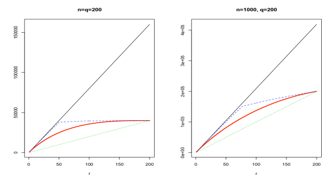
Figure 1. In bold red $r\to\mathcal{S}_{q\times n}(r)^{2}$, in solid black $r\to r\,(\sqrt{n}+\sqrt{q})^{2}$, in dashed blue the upper-bound of Lemma 1, in dotted green the lower bound. Left: $q=n=200$. Right: $q=200$ and $n=1000$.

Finally, for large values of $q$ and $n$, asymptotics formulaes for $\mathcal{S}_{q\times n}(r)$ can be useful. It is standard that when $n,q$ go to infinity with $q/n\to\beta\leq 1$, the empirical distribution of the eigenvalues of $n^{-1}G_{q\times n}G_{q\times n}^{*}$ converges almost surely to the the Marchenko-Pastur distribution [18], which has a density on $[(1-\sqrt{\beta})^{2},(1+\sqrt{\beta})^{2}]$ given by

$$f_{\beta}(x)={1\over 2\pi\beta x}\,\sqrt{\big{(}x-(1-\sqrt{\beta})^{2}\big{)}\big{(}(1+\sqrt{\beta})^{2}-x\big{)}}.$$

As a consequence, when $q$ and $n$ go to infinity with $q/n\to\beta\leq 1$ and $r/q\to\alpha\leq 1$, we have

(4) $$\mathcal{S}_{q\times n}(r)^{2}\sim nq\int_{x_{\alpha}}^{(1+\sqrt{\beta})^{2}}xf_{\beta}(x)\,dx,$$

where $x_{\alpha}$ is defined by

$$\int_{x_{\alpha}}^{(1+\sqrt{\beta})^{2}}f_{\beta}(x)\,dx=\alpha.$$

Since the role of $q$ and $n$ is symmetric, the same result holds when $n/q\to\beta\leq 1$ and $r/n\to\alpha\leq 1$. This approximation (4) can be evaluated efficiently (see the Appendix) and it turns to be a very accurate approximation of $\mathcal{S}_{q\times n}(r)$ for $n,q$ large enough (say $nq>1000$).

2.2. Computation of $X\hat{A}_{r}$

Next lemma provides a useful formula for $X\hat{A}_{r}$.

Lemma 2.

Write $P$ for the projection matrix $P=X(X^{*}X)^{+}X^{*}$, with $(X^{*}X)^{+}$ the Moore-Penrose pseudo-inverse of $X^{*}X$. Then, for any $r\leq q$ we have $X\widehat{A}_{r}=(PY)_{r}$ where $(PY)_{r}$ minimizes $\|PY-B\|^{2}$ over the matrices $B$ of rank at most $r$.

As a consequence, writing $PY=U\Sigma V^{*}$ for the singular value decomposition of $PY$, the matrix $X\hat{A}_{r}$ is given by $X\hat{A}_{r}=U\Sigma_{r}V^{*}$, where $\Sigma_{r}$ is obtained from $\Sigma$ by setting $(\Sigma_{r})_{i,i}=0$ for $i\geq r+1$.

Proof of Lemma 2. We note that $\|PY-P(PY)_{r}\|^{2}\leq\|PY-(PY)_{r}\|^{2}$ and rank$(P(PY)_{r})\leq r$, so $P(PY)_{r}=(PY)_{r}$. In particular, we have $(PY)_{r}=X\tilde{A}_{r}$, with $\tilde{A}_{r}=(X^{*}X)^{+}X^{*}(PY)_{r}$. Since the rank of $X\widehat{A}_{r}$ is also at most $r$, we have

$$\|Y-X\tilde{A}_{r}\|^{2} = \|Y-PY\|^{2}+\|PY-(PY)_{r}\|^{2}$$

$$\leq \|Y-PY\|^{2}+\|PY-X\widehat{A}_{r}\|^{2}=\|Y-X\widehat{A}_{r}\|^{2}.$$

Since the rank of $\tilde{A}_{r}$ is not larger than $r$, we then have $\tilde{A}_{r}=\hat{A}_{r}$.

3. The case of known variance

In this section we revisit the results of Bunea et al. [7, 8] for the case where $\sigma^{2}$ is known. This analysis will give us a benchmark for the case of unknown variance. Next theorem states an oracle inequality for the selection Criterion (2) with penalty fulfilling ${\mathrm{pen}}_{\sigma^{2}}(r)\geq K\mathcal{S}_{q\times n}(r)^{2}$ for $K>1$. Later on, we will prove that the penalty ${\mathrm{pen}}_{\sigma^{2}}(r)=\mathcal{S}_{q\times n}(r)^{2}$ is minimal in some sense.

Theorem 1.

Assume that for some $K>1$ we have

(5) $${\mathrm{pen}}_{\sigma^{2}}(r)\geq K\mathcal{S}_{q\times n}(r)^{2}\quad\textrm{for all }\ \ r\leq\min(n,q).$$

Then, when $\hat{r}$ is selected by minimizing (2) the estimator $\widehat{A}=\widehat{A}_{\hat{r}}$ satisfies

(6) $${\mathbb{E}}\left[{\|X\widehat{A}-XA\|^{2}}\right]\leq c(K)\,\min_{r}\left\{{{\mathbb{E}}\left[{\|XA-X\widehat{A}_{r}\|^{2}}\right]+{\mathrm{pen}}_{\sigma^{2}}(r)\sigma^{2}+\sigma^{2}}\right\}$$

for some positive constant $c(K)$ depending on $K$ only.

The risk bound (6) ensures that the risk of the estimator $\widehat{A}$ is not larger (up to a constant) than the minimum over $r$ of the sum of the risk of the estimator $\widehat{A}_{r}$ plus the penalty term ${\mathrm{pen}}_{\sigma^{2}}(r)\sigma^{2}$. We will see below that this ensures that the estimator $\widehat{A}$ is adaptive minimax.

For $r\ll\min(n,q)$, the penalty ${\mathrm{pen}}_{\sigma^{2}}(r)=K\mathcal{S}_{q\times n}(r)^{2}$ is close to the penalty ${\mathrm{pen}}^{\prime}_{\sigma^{2}}=K(\sqrt{q}+\sqrt{n})^{2}r$ proposed by Bunea et al. [8], but ${\mathrm{pen}}_{\sigma^{2}}(r)$ can be significantly smaller than ${\mathrm{pen}}^{\prime}_{\sigma^{2}}(r)$ for moderate values of $r$, see Figure 1. Next proposition shows that choosing a penalty ${\mathrm{pen}}_{\sigma^{2}}(r)=K\mathcal{S}_{q\times n}(r)^{2}$ with $K<1$ can lead to a strong overfitting.

Proposition 1.

Assume that $A=0$ and that $\hat{r}$ is any minimizer of the Criterion (2) with ${\mathrm{pen}}_{\sigma^{2}}(r)=K\mathcal{S}_{q\times n}(r)^{2}$ for some $K<1$. Then, setting $\alpha=1-\sqrt{(1+K)/2}>0$ we have

$$\mathbb{P}\left({\hat{r}\geq{1-K\over 4}\times{nq-1\over(\sqrt{n}+\sqrt{q})^{2}}}\right)\geq 1-e^{\alpha^{2}/2}\,{e^{-\alpha^{2}\max(n,q)/2}\over 1-e^{-\alpha^{2}\max(n,q)/2}}\,.$$

As a consequence, the risk bound (6) cannot hold when Condition (5) is replaced by ${\mathrm{pen}}_{\sigma^{2}}(r)=K\mathcal{S}_{q\times n}(r)^{2}$ with $K<1$.

In the sense of Birgé and Massart [5], the Condition (5) is therefore minimal.

Minimax adaptation

Fact 1.

For any $\rho\in\,]0,1]$, there exists a constant $c_{\rho}>0$ such that for any integers $m,n,p$ larger than 2, any positive integer $q$ less than $\min(m,p)$ and any design matrix $X$ fulfilling

(7) $$\sigma_{q}(X)\geq\rho\,\sigma_{1}(X),\quad\textrm{where}\ \ q=\textrm{rank}(X),$$

we have

$$\inf_{\tilde{A}}\sup_{A\,:\,\mathrm{rank}(A)\leq r}{\mathbb{E}}\left[{\|X\tilde{A}-XA\|^{2}}\right]\geq c_{\rho}(q+n)r\sigma^{2},\quad\textrm{for all}\ \ r\leq\min(n,q).$$

When $p\leq m$ and $q=p$, this minimax bound follows directly from Theorem 5 in Rohde and Tsybakov [20] as noticed by Bunea et al., see [8] Section 2.3 Remark (ii) for a slightly different statment of this bound. We refer to Section 7.7 for a proof of the general case (with possibly $q<p$ and/or $p>m$).

If we choose ${\mathrm{pen}}_{\sigma^{2}}(r)=K\mathcal{S}_{q\times n}(r)^{2}$ for some $K>1$, we have ${\mathrm{pen}}_{\sigma^{2}}(r)\leq 2Kr(q+n)$ according to Lemma 1. The risk bound (6) then ensures that our estimator $\widehat{A}$ is adaptive minimax (as is the estimator proposed by Bunea et al.).

4. The case of unknown variance

We present now our main result which provides a selection criterion for the case where the variance $\sigma^{2}$ is unknown. For a given $r_{\max}\leq\min(n,q)$, we propose to select $\hat{r}\in\left\{{1,\ldots,r_{\max}}\right\}$ by minimizing over $\left\{{1,\ldots,r_{\max}}\right\}$ Criterion (3), namely

$${\mathrm{Crit}}(r)=\log(\|Y-X\widehat{A}_{r}\|^{2})+{\mathrm{pen}}(r).$$

We note that the Criterion (3) is equivalent to the criterion

(8) $${\mathrm{Crit}}^{\prime}(r)=\|Y-X\widehat{A}_{r}\|^{2}\left({1+{{\mathrm{pen}}^{\prime}(r)\over nm}}\right),$$

with ${\mathrm{pen}}^{\prime}(r)=nm(e^{{\mathrm{pen}}(r)}-1)$. This last criterion bears some similitude with the Criterion (2). Indeed, the Criterion (8) can be written as

$$\|Y-X\widehat{A}_{r}\|^{2}+{\mathrm{pen}}^{\prime}(r)\hat{\sigma}^{2}_{r},$$

with $\hat{\sigma}^{2}_{r}=\|Y-X\widehat{A}_{r}\|^{2}/(nm)$, which is the maximum likelihood estimator of $\sigma^{2}$ associated to $\widehat{A}_{r}$. To facilitate comparisons with the case of known variance, we will work henceforth with the Criterion (8). Next theorem provides an upper bound for the risk of the estimator $X\widehat{A}_{\hat{r}}$.

Theorem 2.

Assume that for some $K>1$ we have both

(9) $$K\mathcal{S}_{q\times n}(r_{\max})^{2}+1<nm$$

(10) $$\textrm{and}\quad{\mathrm{pen}}^{\prime}(r)\geq{K\mathcal{S}_{q\times n}(r)^{2}\over 1-{1\over nm}(1+K\mathcal{S}_{q\times n}(r)^{2})},\quad\textrm{for}\ r\leq r_{\max}.$$

Then, when $\hat{r}$ is selected by minimizing (8) over $\left\{{1,\ldots,r_{\max}}\right\}$, the estimator $\widehat{A}=\widehat{A}_{\hat{r}}$ satisfies

(11) $${\mathbb{E}}\left[{\|X\widehat{A}-XA\|^{2}}\right]\\ \leq c(K)\,\min_{r\leq r_{\max}}\left\{{{\mathbb{E}}\left[{\|X\widehat{A}_{r}-XA\|^{2}}\right]\left({1+{{\mathrm{pen}}^{\prime}(r)\over nm}}\right)+({\mathrm{pen}}^{\prime}(r)+1)\sigma^{2}}\right\}.$$

for some constant $c(K)>0$ depending only on $K$.

Let us compare Theorem 2 with Theorem 1. The two main differences lie in Condition (10) and in the form of the risk bound (11). Condition (10) is more stringent than Condition (5). More precisely, when $r$ is small compared to $q$ and $n$, both conditions are close, but when $r$ is of a size comparable to $q$ or $n$, Condition (10) is much stronger than (5). In the case where $m=q$, it even enforces a blow up of the penalty ${\mathrm{pen}}^{\prime}(r)$ when $r$ tends to $\min(n,m)$. This blow up is actually necessary to avoid overfitting since, in this case, the residual sum of squares $\|Y-X\widehat{A}_{r}\|^{2}$ tends to 0 when $r$ increases. The second major difference between Theorem 2 and Theorem 1 lies in the multiplicative factor $(1+{\mathrm{pen}}^{\prime}(r)/nm)$ in the right-hand side of the risk bound (11). Due to this term, the bound (11) is not (strictly speaking) an oracle bound. To obtain an oracle bound, we have to add a condition on $r_{\max}$ to ensure that ${\mathrm{pen}}^{\prime}(r)\leq Cnm$ for all $r\leq r_{\max}$. Next corollary provides such a condition.

Corollary 1.

Assume that

(12) $$r_{\max}\leq\alpha\,{nm-1\over K(\sqrt{q}+\sqrt{n})^{2}}\quad\textrm{for some }\ 0<\alpha<1,$$

and set

$${\mathrm{pen}}(r)=-\log(1-K\mathcal{S}_{q\times n}(r)^{2}/(nm-1))\quad\textrm{for some }K>1.$$

Then, there exists $c(K,\alpha)>0$ such that, when $\hat{r}$ is selected by minimizing (3) over $\left\{{1,\ldots,r_{\max}}\right\}$, we have the oracle inequality

$${\mathbb{E}}\left[{\|X\widehat{A}-XA\|^{2}}\right]\\ \leq c(K,\alpha)\,\min_{r\leq r_{\max}}\left\{{{\mathbb{E}}\left[{\|X\widehat{A}_{r}-XA\|^{2}}\right]+r(\sqrt{n}+\sqrt{q})^{2}\sigma^{2}+\sigma^{2}}\right\}.$$

In particular, the estimator $\widehat{A}$ is adaptive minimax up to the rank $r_{\max}$ specified by (12). In the worst case where $m=q$, Condition (12) requires that $r_{\max}$ remains smaller than a fraction of $\min(n,q)$. In the more favorable case where $m$ is larger than $4q$, Condition (12) can be met with $r_{\max}=\min(q,n)$ for suitable choices of $K$ and $\alpha$.

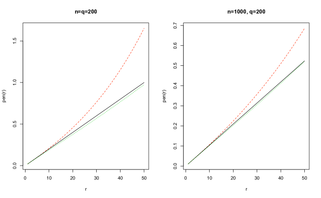
Figure 2. In dotted green ${\mathrm{pen}}(r)=-\log(1-\mathcal{S}_{q\times n}(r)^{2}/(nq-1))$, in solid black ${\mathrm{pen}}(r)=r\,(\sqrt{n}+\sqrt{q})^{2}/(nq)$, in dashed red ${\mathrm{pen}}^{\prime}(r)/(nq)=\mathcal{S}_{q\times n}(r)^{2}/(nq-1-\mathcal{S}_{q\times n}(r)^{2})$. Left : $q=n=200$. Right : $q=200$ and $n=1000$.

Let us discuss now in more details the Conditions (9) and (10) of Theorem 2. We have $\mathcal{S}_{q\times n}(r)^{2}<{r(\sqrt{n}+\sqrt{q})^{2}}$ so the Conditions (9) and (10) are satisfied as soon as

$$r_{\max}\leq{nm-1\over K(\sqrt{n}+\sqrt{q})^{2}}\quad\textrm{and}\quad\ {\mathrm{pen}}^{\prime}(r)\geq{Kr(\sqrt{n}+\sqrt{q})^{2}\over 1-{1\over nm}(1+Kr(\sqrt{n}+\sqrt{q})^{2})},\quad\textrm{for }r\leq r_{\max}.$$

In terms of the Criterion (3), the Condition (10) reads

$${\mathrm{pen}}(r)\geq-\log(1-K\mathcal{S}_{q\times n}(r)^{2}/(nm-1)).$$

When ${\mathrm{pen}}(r)$ is defined by taking equality in the above inequality, we have ${\mathrm{pen}}(r)\approx Kr(\sqrt{n}+\sqrt{q})^{2}/(nm)$ for small values of $r$, see Figure 2.

Finally, next proposition, shows that the Condition (10) on ${\mathrm{pen}}^{\prime}(r)$ is necessary to avoid overfitting.

Proposition 2.

Assume that $A=0$ and that $\hat{r}$ is any minimizer of Criterion (8) over $\left\{{1,\ldots,\min(n,q)-1}\right\}$ with

(13) $${\mathrm{pen}}^{\prime}(r)={K\mathcal{S}_{q\times n}(r)^{2}\over 1-{K\over nm}\mathcal{S}_{q\times n}(r)^{2}}\quad\textrm{for some}\ K<1.$$

Then, setting $\alpha=(1-K)/4>0$ we have

$$\mathbb{P}\left({\hat{r}\geq{1-K\over 8}\times{nq-1\over(\sqrt{n}+\sqrt{q})^{2}}}\right)\geq 1-2e^{\alpha^{2}/2}{e^{-\alpha^{2}\max(n,q)/2}\over 1-e^{-\alpha^{2}\max(n,q)/2}}\,.$$

As in Proposition 1, a consequence of Proposition 2 is that Theorem 2 cannot hold with Condition (10) replaced by (13). Condition (10) is then minimal in the sense of Birgé and Massart [5].

5. Comments and extensions

5.1. Link with PCA

In the case where $X$ is the identity matrix, namely $Y=A+E$, Principal Component Analysis (PCA) is a popular technique to estimate $A$. The matrix $A$ is estimated by projecting the data $Y$ on the $r$ first principal components, the number $r$ of components being chosen according to empirical or asymptotical criterions.

It turns out that the projection of the data $Y$ on the $r$ first principal components coincides with the estimator $\widehat{A}_{r}$. The criterion (3) then provides a theoretically grounded way to select the number $r$ of components. Theorem 2 ensures that the risk of the final estimate $\widehat{A}_{\hat{r}}$ nearly achieves the minimum over $r$ of the risks ${\mathbb{E}}\left[{\|\hat{A}_{r}-A\|^{2}}\right]$.

5.2. Sub-Gaussian errors

We have considered for simplicity the case of Gaussian errors, but the results can be extended to the case where the entries $E_{i,j}$ are i.i.d sub-Gaussian. In this case, the matrix $PE$ will play the role of the matrix $G_{q\times n}$ in the Gaussian case. More precisely, combining recent results of Rudelson and Vershynin [21] and Bunea et al. [7] on sub-Gaussian random matrices, with concentration inequality for sub-Gaussian random variables [16] enables to prove an analog of Lemma 1 for ${\mathbb{E}}\left[{\|PE\|_{(2,r)}}\right]^{2}$ (with different constants). Then, the proof of Theorem 1 and Theorem 2 can be easily adapted, replacing the Condition (5) by

$${\mathrm{pen}}(r)\geq K{\mathbb{E}}\left[{\|PE\|_{(2,r)}}\right]^{2},\quad\textrm{for }r\leq\min(q,n),$$

and the Conditions (9) and (10) by $K{\mathbb{E}}\left[{\|PE\|_{(2,r_{\max})}}\right]^{2}<{\mathbb{E}}[\|E\|]^{2}$ and

$${\mathrm{pen}}^{\prime}(r)\geq{K{\mathbb{E}}\left[{\|PE\|_{(2,r)}}\right]^{2}\over 1-K{\mathbb{E}}\left[{\|PE\|_{(2,r)}}\right]^{2}/\,{\mathbb{E}}\left[{\|E\|}\right]^{2}},\quad\textrm{for}\ r\leq r_{\max}.$$

Analogs of Proposition 1 and 2 also hold with different constants.

5.3. Selecting among arbitrary estimators

Our theory provides a procedure to select among the family of estimators $\{\widehat{A}_{r},\ r\leq r_{\max}\}$. It turns out that it can be extended to arbitrary (finite) families of estimators $\{A_{\lambda},\ \lambda\in\Lambda\}$ such as the nuclear norm penalized estimator family $\{\widehat{A}_{\lambda}^{\ell_{1}},\lambda\in\Lambda\}$. The most straightforward way is to replace everywhere $\widehat{A}_{r}$ by $\widehat{A}_{\lambda}$ and ${\mathrm{pen}}(r)$ by $\underline{{\mathrm{pen}}}(\lambda)$, with $\underline{{\mathrm{pen}}}(\lambda)={\mathrm{pen}}(\textrm{rank}(\widehat{A}_{\lambda})).$ In the spirit of Baraud et al. [4], we may also consider more refined criterions such as

$${\mathrm{Crit}}_{\alpha}(\lambda)=\min_{r\leq r_{\max}}\left\{{(\|Y-X\widehat{A}_{\lambda,r}\|^{2}+\|X\widehat{A}_{\lambda}-X\widehat{A}_{\lambda,r}\|^{2})\left({1+{{\mathrm{pen}}^{\prime}(r)\over nm}}\right)}\right\},$$

where $\alpha>0$ and $\widehat{A}_{\lambda,r}$ minimizes $\|B-\widehat{A}_{\lambda}\|$ over the matrices $B$ of rank at most $r$. Analogs of Theorem 2 can be derived for such criterions, but we will not pursue in that direction.

6. Numerical experiments

We perform numerical experiments on synthetic data in two different settings. In the first experiment, we consider a favorable setting where the sample size $m$ is large compared to the number $p$ of covariables. In the second experiment, we consider a more challenging setting where the sample size $m$ is small compared to $p$. The objectives of our experiments are mainly:

• to give an example of implementation of our procedure,

• to demonstrate that it can handle high-dimensional settings.

Simulation setting

Our experiments are inspired by those of Bunea et al. [7, 8], the main difference is that we work in higher dimensions. The simulation design is the following. The rows of the matrix $X$ are drawn independently according to a centered Gaussian distribution with covariance matrix $\Sigma_{i,j}=\rho^{|i-j|}$, $\rho>0$. For a positive $b$, the matrix $A$ is given by $A=bB_{p\times r}B_{r\times n}$, where the entries of the $B$ matrices are i.i.d. standard Gaussian. For $r\leq\min(n,p)$, the rank of the matrix $A$ is then $r$ with probability one and the rank of $X$ is $\min(m,p)$ a.s.

Experiment 1:

in the first experiment, we consider a case where the sample size $m=400$ is large compared to the number $p=100$ of covariables and $n=100$. The other parameters are $r=40$, $\rho$ varies in $\{0.1,0.5,0.9\}$ and $b$ varies in $\{0.025,0.05,0.075,0.1\}$. This experiment is actually the same as the Experiment 1 in [8], except that we have multiplied $m,\ p,\ n,\ r$ by four and adjusted the values of $b$.

Experiment 2:

the second experiment is much more challenging since the sample size $m=100$ is small compared to the number $p=500$ of covariables and $n=500$. Furthermore, the rank $q$ of $X$ equals $m$, which is the least-favorable case for estimating the variance. For the other parameters, we set $r=20$, $\rho$ varies in $\{0.1,0.5,0.9\}$ and $b$ varies in $\{0.005,0.01,0.015,0.02\}$.

Estimators

For $K>1$, we write $\mathrm{K\!F}[K]$ for the estimator $\widehat{A}_{\hat{r}}$ with $\hat{r}$ selected by the Criterion (8) with

$${\mathrm{pen}}^{\prime}(r)={K\mathcal{S}_{q\times n}(r)^{2}\over 1-{1\over nm}(1+K\mathcal{S}_{q\times n}(r)^{2})}$$

(the notation $\mathrm{K\!F}$ refers to the Ky-Fan norms involved in $\mathcal{S}_{q\times n}(r)$).

For $\lambda>0$, we write $\mathrm{RSC}[\lambda]$ for the estimator $\widehat{A}_{\hat{r}}$ with $\hat{r}$ selected by the criterion introduced by Bunea, She and Wegkamp [7]

$${\mathrm{Crit}}_{\lambda}(r)=\|Y-X\widehat{A}_{r}\|^{2}+\lambda(n+\textrm{rank}(X))r.$$

Bunea et al. [8] proposes to use $\lambda=K\hat{\sigma}^{2}$ with $K\geq 2$ and

$$\hat{\sigma}^{2}={\|Y-PY\|^{2}\over mn-n\textrm{rank}(X)},\quad\textrm{with $P$ the projector onto the range of }X.$$

We denote by $\mathrm{RSCI}[K]$ the resulting estimator $\mathrm{RSC}[K\hat{\sigma}^{2}]$.

Both procedures $\mathrm{K\!F}$ and $\mathrm{RSCI}$ depend on a tuning parameter $K$. There is no reason for the existence of a universal ”optimal” constant $K$. Nevertheless, Birgé and Massart [5] suggest to penalize by twice the minimal penalty, which corresponds to the choice $K=2$ for $\mathrm{K\!F}$. The value $K=2$ is also the value recommended by Bunea et al. [8] Section 4 for the $\mathrm{RSCI}$ (see the ”adaptive tuning parameter” $\mu_{adapt}$). Another classical approach for choosing a tuning parameter is Cross-Validation : for example, $K$ can be selected among a small grid of values between 1 and 3 by $V$-Fold CV. We emphasize that there is no theoretical justification that Cross-Validation will choose the best value for $K$. Nevertheless, for each value $K$ in the grid, the estimators $\mathrm{K\!F}[K]$ and $\mathrm{RSCI}[K]$ fulfills an oracle inequality with large probability, so the estimators with $K$ chosen by CV will also fulfills an oracle inequality with large probability (as long as the size of the grid remains small). We will write $\mathrm{K\!F}[K\!=\!CV]$ and $\mathrm{RSCI}[K\!=\!CV]$ for the estimators $\mathrm{K\!F}$ and $\mathrm{RSCI}$ with $K$ selected by $10$-fold Cross-Validation.

Finally, in Experiment 2 the estimator $\mathrm{RSCI}$ cannot be implemented since rank$(X)=m$. Yet, it is still possible to implement the procedure $\mathrm{RSC}[\lambda]$ and select $\lambda>0$ among a large grid of values by 10-fold Cross-Validation, even if in this case there is no theoretical control on the risk of the resulting estimator $\mathrm{RSC}[\lambda\!=\!CV]$. We will use this estimator as a benchmark in Experiment 2.

Results

The results of the first experiment are reported in Figure 3 and those of the second experiment in Figure 4. The boxplots of the first line compare the performances of estimators $\mathrm{K\!F}$ and $\mathrm{RSCI}$ to that of the estimator $X\widehat{A}_{r}$ that we would use if we knew that the rank of A is $r$. The boxplots give for each value of $\rho$ the distribution of the ratios

(14) $${\|XA-X\widehat{A}\|^{2}\over\|XA-X\widehat{A}_{r}\|^{2}}\ \wedge\ 10$$

for $\widehat{A}$ given by $\mathrm{K\!F}[K\!=\!2]$, $\mathrm{RSCI}[K\!=\!2]$, $\mathrm{K\!F}[K\!=\!CV]$ and $\mathrm{RSCI}[K\!=\!CV]$ in the first experiment and by $\mathrm{K\!F}[K\!=\!2]$, $\mathrm{K\!F}[K\!=\!CV]$, and $\mathrm{RSC}[\lambda\!=\!CV]$ in the second experiment. The ratios (14) are truncated to 10 for a better visualization. Finally, we plot in the second line the mean estimated rank ${\mathbb{E}}[\hat{r}]$ for each estimator and each value of $b$ and $\rho$.

Experiment 1 (large sample size)

All estimators $\mathrm{K\!F}[K\!=\!2]$, $\mathrm{RSCI}[K\!=\!2]$, $\mathrm{K\!F}[K\!=\!CV]$ and $\mathrm{RSCI}[K\!=\!CV]$ perform very similarly and almost all the ratios (14) are equal to 1.

Experiment 2 (small sample size)

The estimator $\mathrm{K\!F}[K\!=\!CV]$ has global good performances, with a median ratio (14) around 1, but the ratio (14) can be as high as 5 in some examples for $\rho=0.9$. In contrast, the estimator $\mathrm{K\!F}[K\!=\!2]$ is very stable but it has a median value significantly above the other methods. Finally, the performances of the estimator $\mathrm{RSC}[\lambda\!=\!CV]$ are very contrasted. For small correlation ($\rho=0.1$), its performances are similar to that of $\mathrm{K\!F}[K\!=\!CV]$. For $\rho=0.5$ or $\rho=0.9$, it has very good performances most of the time (similar to $\mathrm{K\!F}[K\!=\!CV]$) but it completely fails on a small fraction of examples. For example, for $\rho=0.9$, it has a ratio (14) smaller than $7$ in 80% of the examples (with a median value close to 1), but in 20% of the examples, it completely fails and the ratio $\|XA-X\widehat{A}\|^{2}/\|XA-X\widehat{A}_{r}\|^{2}$ for $\mathrm{RSC}[\lambda\!=\!CV]$ can be has high as $10^{13}$ (these values do not appear in Figure 4 since we have truncated the ratio (14) to 10 to avoid a complete shrinkage of the boxplots). We recall, that there exists no risk bound for the estimator $\mathrm{RSC}[\lambda\!=\!CV]$, so these results are not in contradiction with any theory.

Finally, we emphasize that no conclusion should be drawn from these two single experiments about the superiority of one procedure over the others.

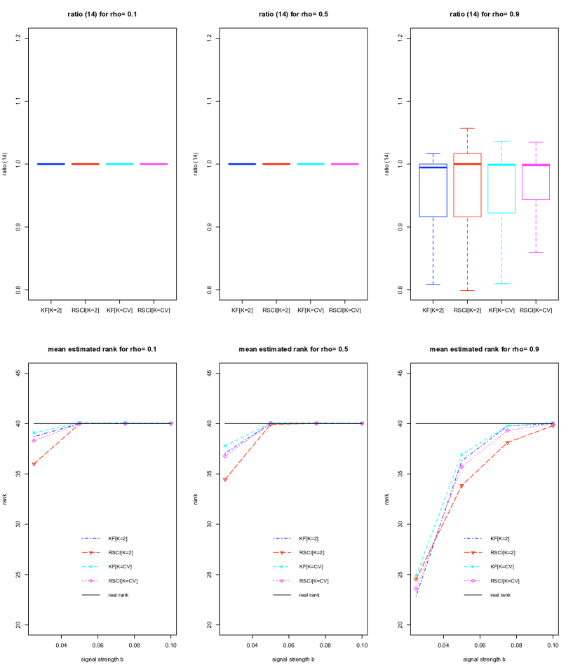
Figure 3. Experiment 1. Left to right : $\rho=0.1,\,0.5,\,0.9$. Top : boxplots of the ratio (14) for $\mathrm{K\!F}[K\!=\!2]$, $\mathrm{RSCI}[K\!=\!2]$, $\mathrm{K\!F}[K\!=\!CV]$ and $\mathrm{RSCI}[K\!=\!CV]$. Bottom : mean estimated rank ${\mathbb{E}}[\hat{r}]$ for each estimator and each value of $b$.

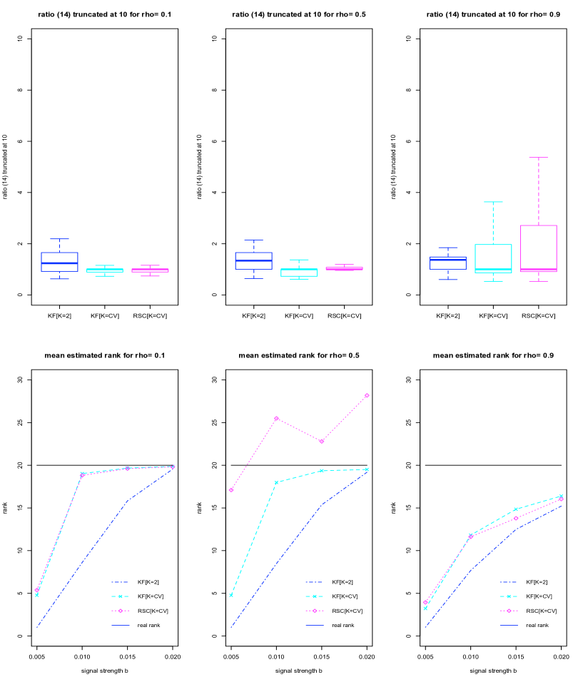
Figure 4. Experiment 2. Left to right : $\rho=0.1,\,0.5,\,0.9$. Top : boxplots of the ratio (14) truncated at 10 for $\mathrm{K\!F}[K\!=\!2]$, $\mathrm{K\!F}[K\!=\!CV]$ and $\mathrm{RSC}[\lambda\!=\!CV]$. Bottom : mean estimated rank ${\mathbb{E}}[\hat{r}]$ for each estimator and each value of $b$.

7. Proof of the mains results

7.1. Proof of Lemma 1

For notational simplicity we write $G=G_{q\times n}$. The case $r=1$ follows from Slepian’s Lemma, see Davidson and Szarek [9] Chapter 8. For $r>1$, we note that

$${\mathbb{E}}\left[{\|G\|_{(2,r)}}\right]^{2}\leq\min\left\{{r\,{\mathbb{E}}\left[{\|G\|_{(2,1)}}\right]^{2}\,,\sum_{k=1}^{r}{\mathbb{E}}[\sigma_{k}^{2}(G)]}\right\}.$$

The first upper bound $\mathcal{S}_{q\times n}(r)^{2}\leq r(\sqrt{n}+\sqrt{q})^{2}$ follows. For the second upper bound, we note that

$$\sum_{k=1}^{r}{\mathbb{E}}[\sigma_{k}^{2}(G)]\leq{\mathbb{E}}[\|G\|^{2}]-\sum_{k=r+1}^{q}{\mathbb{E}}[\sigma_{k}(G)]^{2}.$$

The interlacing inequalities [12] ensure that $\sigma_{k}(G_{k}^{\prime})\leq\sigma_{k}(G)$ where $G_{k}^{\prime}$ is the matrix made of the $k$ first rows of $G$. The second bound then follows from ${\mathbb{E}}[\sigma_{k}(G_{k}^{\prime})]\geq\sqrt{n}-\sqrt{k}$, see [9].

Let us turn to the third bound. The map $G\to\sigma_{k}(G)$ is 1-Lipschitz so, writing $M_{k}$ for the median of $\sigma_{k}$, the concentration inequality for Gaussian random variables ensures that $(M_{k}-\sigma_{k}(G))_{+}\leq\xi_{+}$ and $(\sigma_{k}(G)-M_{k})_{+}\leq\xi_{+}^{\prime}$ where $\xi_{+}$ and $\xi_{+}^{\prime}$ are the positive part of two standard Gaussian random variables. As a consequence we have

$${\mathbb{E}}[\sigma_{k}^{2}(G)]-{\mathbb{E}}[\sigma_{k}(G)]^{2}+(M_{k}-{\mathbb{E}}[\sigma_{k}(G)])^{2} = {\mathbb{E}}\left[{(\sigma_{k}(G)-M_{k})_{+}^{2}}\right]+{\mathbb{E}}\left[{(M_{k}-\sigma_{k}(G))_{+}^{2}}\right]$$

$$\leq {\mathbb{E}}[\xi_{+}^{{}^{\prime}2}]+{\mathbb{E}}[\xi_{+}^{2}]=1,$$

and thus ${\mathbb{E}}[\sigma_{k}^{2}(G)]\leq{\mathbb{E}}[\sigma_{k}(G)]^{2}+1$.

Furthermore, the interlacing inequalities [12] ensure that $\sigma_{k}(G)\leq\sigma_{1}(G_{q-k+1}^{\prime})$. We can then bound ${\mathbb{E}}[\sigma_{k}(G)]$ by

$${\mathbb{E}}[\sigma_{k}(G)]\leq\sqrt{n}+\sqrt{q-k+1}$$

which leads to the last upper bound.

For the lower bound, we start from $\|G\|_{(2,r)}^{2}\geq\|G\|^{2}r/q$ (sum of a decreasing sequence) and use again the Gaussian concentration inequality to get

$${\mathbb{E}}[\|G\|^{2}]-1=nq-1\leq{\mathbb{E}}[\|G\|]^{2}$$

and concludes that $r(nq-1)/q\leq{\mathbb{E}}\left[{\|G\|_{(2,r)}}\right]^{2}=\mathcal{S}_{q\times n}(r)^{2}$.

7.2. A technical lemma

Next lemma provides a control of the size of the scalar product $<E,X\widehat{A}_{k}-XA_{r}>$ which will be useful for the proofs of Theorem 1 and Theorem 2.

Lemma 3.

Fix $r\leq\min(n,q)$ and write $A_{r}$ for the best approximation of $A$ with rank at most $r$. Then, there exists a random variable $U_{r}$ such that ${\mathbb{E}}(U_{r})\leq r\min(n,q)$ and for any $\eta>0$ and all $k\leq\min(n,q)$

$$2\sigma\,|<E,X\widehat{A}_{k}-XA_{r}>| \leq {1\over 1+\eta}\|X\widehat{A}_{k}-XA\|^{2}+{1+1/\eta\over(1+\eta)^{2}}\|XA-XA_{r}\|^{2}$$

$$\ +\,(1+\eta)^{2}(1+1/\eta)\sigma^{2}U_{r}+(1+\eta)^{3}\sigma^{2}\|PE\|_{(2,k)}^{2}$$

where $P=X(X^{*}X)^{+}X^{*}$ is as in Lemma 1.

Iterating twice the inequality $2ab\leq a^{2}/c+cb^{2}$ gives

$$2\sigma\,|<E,X\widehat{A}_{k}-XA_{r}>|\\ \leq{1\over 1+\eta}\|X\widehat{A}_{k}-XA\|^{2}+{1+1/\eta\over(1+\eta)^{2}}\|XA-XA_{r}\|^{2}+(1+\eta)^{2}\sigma^{2}{<E,X\widehat{A}_{k}-XA_{r}>^{2}\over\|X\widehat{A}_{k}-XA_{r}\|^{2}}.$$

We write $XA_{r}=U\Gamma_{r}V^{*}$ for the singular value decomposition of $XA_{r}$, with the convention that the diagonal entries of $\Gamma_{r}$ are decreasing. Since the rank of $XA_{r}$ is upper bounded by the rank of $A_{r}$, the $m\times n$ diagonal matrix $\Gamma_{r}$ has at most $r$ non zeros elements. Assume first that $n\leq q$. Denoting by $I_{r}$ the $m\times m$ diagonal matrix with $(I_{r})_{i,i}=1$ if $i\leq r$ and $(I_{r})_{i,i}=0$ if $i>r$ and writing $I_{-r}=I-I_{r}$ and $\widehat{B}_{k}=U^{*}X\widehat{A}_{k}V$, we have

$${<E,X\widehat{A}_{k}-XA_{r}>^{2}\over\|X\widehat{A}_{k}-XA_{r}\|^{2}} = {<U^{*}PEV,\widehat{B}_{k}-\Gamma_{r}>^{2}\over\|\widehat{B}_{k}-\Gamma_{r}\|^{2}}$$

$$= {\left({<U^{*}PEV,I_{r}(\widehat{B}_{k}-\Gamma_{r})>+<U^{*}PEV,I_{-r}\widehat{B}_{k}>}\right)^{2}\over\|I_{r}(\widehat{B}_{k}-\Gamma_{r})\|^{2}+\|I_{-r}\widehat{B}_{k}\|^{2}}$$

$$\leq (1+\eta^{-1}){<U^{*}PEV,I_{r}(\widehat{B}_{k}-\Gamma_{r})>^{2}\over\|I_{r}(\widehat{B}_{k}-\Gamma_{r})\|^{2}}+(1+\eta){<U^{*}PEV,I_{-r}\widehat{B}_{k}>^{2}\over\|I_{-r}\widehat{B}_{k}\|^{2}}.$$

The first term is upper bounded by

$${<U^{*}PEV,I_{r}(\widehat{B}_{k}-\Gamma_{r})>^{2}\over\|I_{r}(\widehat{B}_{k}-\Gamma_{r})\|^{2}}\leq\|I_{r}U^{*}PEV\|^{2}=U_{r}$$

and the expected value of the right-hand side fulfills

$${\mathbb{E}}(U_{r})=n\|I_{r}U^{*}PU\|^{2}=n\|U^{*}PUI_{r}\|^{2}\leq nr.$$

Since the rank of $I_{-r}\widehat{B}_{k}$ is at most $k$, the second term can be bounded by

$${<U^{*}PEV,I_{-r}\widehat{B}_{k}>^{2}\over\|I_{-r}\widehat{B}_{k}\|^{2}}\leq\sup_{\mathrm{rank}(B)\leq k}{<U^{*}PEV,B>^{2}\over\|B\|^{2}}=\|U^{*}PEV\|_{(2,k)}^{2}=\|PE\|_{(2,k)}^{2}.$$

Putting pieces together gives (3) for $n\leq q$. The case $n>q$ can be treated in the same way, starting from

$$\widehat{B}_{k}-\Gamma_{r}=(\widehat{B}_{k}-\Gamma_{r})I_{r}+\widehat{B}_{k}I_{-r}$$

with $I_{r}$ and $I_{-r}$ two $n\times n$ diagonal matrices defined as above.

7.3. Proof of Theorem 1

The inequality ${\mathrm{Crit}}_{\sigma^{2}}(\hat{r})\leq{\mathrm{Crit}}_{\sigma^{2}}(r)$ gives

(16) $$\|X\widehat{A}-XA\|^{2}\leq\|X\widehat{A}_{r}-XA\|^{2}+{\mathrm{pen}}_{\sigma^{2}}(r)\sigma^{2}+2\sigma<E,X\widehat{A}-X\widehat{A}_{r}>-{\mathrm{pen}}_{\sigma^{2}}(\hat{r})\sigma^{2}.$$

Combining this inequality with Inequality (3) of Lemma 3 with $\eta=((1+K)/2)^{1/3}-1>0$, we obtain

$${\eta\over 1+\eta}\|X\widehat{A}-XA\|^{2} \leq \|X\widehat{A}_{r}-XA\|^{2}+2{1+1/\eta\over(1+\eta)^{2}}\|XA-XA_{r}\|^{2}+2{\mathrm{pen}}_{\sigma^{2}}(r)\sigma^{2}$$

$$\ +2(1+\eta)^{2}(1+\eta^{-1})\sigma^{2}U_{r}+{K+1\over 2}\sigma^{2}\|PE\|_{(2,r)}^{2}-{\mathrm{pen}}_{\sigma^{2}}(r)\sigma^{2}$$

$$\ +\sigma^{2}\sum_{k=1}^{\min(n,q)}\left({{K+1\over 2}\,\|PE\|_{(2,k)}^{2}-{\mathrm{pen}}_{\sigma^{2}}(k)}\right)_{+}.$$

The map $E\to\|PE\|_{(2,k)}$ is 1-Lipschitz and convex, so there exists a standard Gaussian random variable $\xi$ such that $\|PE\|_{(2,k)}\leq{\mathbb{E}}[\|PE\|_{(2,k)}]+\xi_{+}$ and then

$${\mathbb{E}}\left({{K+1\over 2}\,\|PE\|_{(2,k)}^{2}-{\mathrm{pen}}(k)}\right)_{+} \leq {1+K\over 2}{\mathbb{E}}\left({\xi_{+}^{2}+2\xi_{+}{\mathbb{E}}[\|PE\|_{(2,k)}]-{K-1\over K+1}{\mathbb{E}}[\|PE\|_{(2,k)}]^{2}}\right)_{+}$$

$$\leq c_{1}(K)\exp(-c_{2}(K){\mathbb{E}}[\|PE\|_{(2,k)}]^{2}).$$

Since $\|PE\|_{(2,k)}$ is distributed as $\|G_{q\times n}\|_{(2,k)}$, Lemma 1 gives that ${\mathbb{E}}[\|PE\|_{(2,k)}]^{2}\geq k\max(n,q)-1$ and the series

$$\sum_{k=1}^{\min(n,q)}{\mathbb{E}}\left({{K+1\over 2}\,\|PE\|_{(2,k)}^{2}-{\mathrm{pen}}(k)}\right)_{+}$$

can be upper-bounded by $c_{1}(K)e^{c_{2}(K)}\left({1-e^{-c_{2}(K)}}\right)^{-1}e^{-c_{2}(K)\max(n,q)}$. Finally, ${\mathbb{E}}[U_{r}]\leq r\min(n,q)$ is bounded by $1+{\mathrm{pen}}(r)$ and $\|XA-XA_{r}\|^{2}$ is smaller than ${\mathbb{E}}\left[{\|XA-X\widehat{A}_{r}\|^{2}}\right]$, so there exists some constant $c(K)>0$ such that (6) holds.

7.4. Proof of Theorem 2.

To simplify the formulaes, we will note $\overline{{\mathrm{pen}}}(r)={\mathrm{pen}}^{\prime}(r)/(nm)$. The inequality ${\mathrm{Crit}}^{\prime}(\hat{r})\leq{\mathrm{Crit}}^{\prime}(r)$ gives

$$\|X\widehat{A}-XA\|^{2}(1+\overline{{\mathrm{pen}}}(\hat{r}))$$

$$\leq \|Y-X\widehat{A}_{r}\|^{2}-\sigma^{2}(1+\overline{{\mathrm{pen}}}(r))\|E\|^{2}+\overline{{\mathrm{pen}}}(r)\|Y-X\widehat{A}_{r}\|^{2}+\overline{{\mathrm{pen}}}(r)\|E\|^{2}\sigma^{2}$$

$$+2(1+\overline{{\mathrm{pen}}}(\hat{r}))\sigma<E,X\widehat{A}-XA>-\overline{{\mathrm{pen}}}(\hat{r})\|E\|^{2}\sigma^{2}$$

$$\leq \left({2\sigma<E,XA_{r}-X\widehat{A}_{r}>-\overline{{\mathrm{pen}}}(r)\sigma^{2}\|E\|^{2}}\right)_{+}+(1+2\overline{{\mathrm{pen}}}(r))\|XA-X\widehat{A}_{r}\|^{2}+3\overline{{\mathrm{pen}}}(r)\|E\|^{2}$$

$$+(1+\overline{{\mathrm{pen}}}(\hat{r}))\left({2\sigma<E,X\widehat{A}-XA_{r}>-{\overline{{\mathrm{pen}}}(\hat{r})\over 1+\overline{{\mathrm{pen}}}(\hat{r})}\,\|E\|^{2}\sigma^{2}}\right)_{+}+2\sigma\overline{{\mathrm{pen}}}(\hat{r})<E,XA_{r}-XA>.$$

Dividing both side by $1+\overline{{\mathrm{pen}}}(\hat{r})$, we obtain

$$\|X\widehat{A}-XA\|^{2}\leq(1+2\overline{{\mathrm{pen}}}(r))\|XA-X\widehat{A}_{r}\|^{2}+3\overline{{\mathrm{pen}}}(r)\|E\|^{2}+2\sigma|<E,XA-XA_{r}>|+\Delta_{r}+\Delta_{\hat{r}}$$

where

$$\Delta_{k}=\left({2\sigma|<E,X\widehat{A}_{k}-XA_{r}>|-{\overline{{\mathrm{pen}}}(k)\over 1+\overline{{\mathrm{pen}}}(k)}\,\|E\|^{2}\sigma^{2}}\right)_{+}.$$

We first note that ${\mathbb{E}}[\|E\|^{2}]=nm$ and $2\sigma{\mathbb{E}}[|<E,XA-XA_{r}>|]\leq\sigma^{2}+\|XA-XA_{r}\|^{2}$. Then, combining Lemma 3 with $\eta=(K^{1/6}-1)$ and the following lemma with $\delta=\eta$ gives

$${\mathbb{E}}\left[{\|X\widehat{A}-XA\|^{2}}\right]\leq c(K)\left({{\mathbb{E}}\left[{\|XA-X\widehat{A}_{r}\|^{2}}\right](1+\overline{{\mathrm{pen}}}(r))+(1+nm\overline{{\mathrm{pen}}}(r))\sigma^{2}}\right),$$

for some $c(K)>0$.

Lemma 4.

Write $P$ for the projection matrix $P=X(X^{*}X)^{+}X^{*}$, with $(X^{*}X)^{+}$ the Moore-Penrose pseudo-inverse of $X^{*}X$. For any $\delta>0$ and $r\leq\min(n,q)$ such that $(1+\delta){\mathbb{E}}\left[{\|PE\|_{(2,r)}}\right]\leq\sqrt{nm-1}$, we have

(17) $${\mathbb{E}}\left[{(\|PE\|_{(2,r)}^{2}-(1+\delta)^{3}{\mathbb{E}}\left[{\|PE\|_{(2,r)}}\right]^{2}\|E\|^{2}/(nm-1))_{+}}\right]\leq 4\left({1+1/\delta}\right)e^{\delta^{2}/4}e^{-\delta^{2}r\max(n,q)/4}.$$

As a consequence, we have

$${\mathbb{E}}\left[{\sup_{r\leq r_{\max}}\left({\|PE\|_{(2,r)}^{2}-(1+\delta)^{3}\mathcal{S}_{q\times n}(r)^{2}\|E\|^{2}/(nm-1)}\right)_{+}}\right]\\ \leq 4\left({1+1/\delta}\right)e^{\delta^{2}/4}{e^{-\delta^{2}\max(n,q)/4}\over 1-e^{-\delta^{2}\max(n,q)/4}}\,.$$

Proof of the Lemma.

Writing $t=(1+\delta){\mathbb{E}}[\|PE\|_{(2,r)}]/{\mathbb{E}}[\|E\|]\leq 1$, the map $E\to\|PE\|_{(2,r)}-t\|E\|$ is $\sqrt{2}$-Lipschitz. Gaussian concentration inequality then ensures that

$$\|PE\|_{(2,r)} \leq t\|E\|+{\mathbb{E}}[\|PE\|_{(2,r)}-t\|E\|]+2\sqrt{\xi}$$

$$\leq t\|E\|+\left({2\sqrt{\xi}-\delta\,{\mathbb{E}}[\|PE\|_{(2,r)}]}\right)_{+},$$

with $\xi$ a standard exponential random variable. We then get that

$$\|PE\|_{(2,r)}^{2}\leq(1+\delta)t^{2}\|E\|^{2}+4(1+1/\delta)\left({\sqrt{\xi}-\delta\,{\mathbb{E}}[\|PE\|_{(2,r)}]/2}\right)_{+}^{2}$$

and

$${\mathbb{E}}\left[{(\|PE\|_{(2,r)}^{2}-(1+\delta)t^{2}\|E\|^{2})_{+}}\right] \leq 4(1+1/\delta){\mathbb{E}}\left[{\left({\sqrt{\xi}-\delta\,{\mathbb{E}}[\|PE\|_{(2,r)}]/2}\right)_{+}^{2}}\right]$$

$$\leq 4\left({1+1/\delta}\right)e^{-\delta^{2}{\mathbb{E}}[\|PE\|_{(2,r)}]^{2}/4}.$$

The bound (17) then follows from ${\mathbb{E}}[\|PE\|_{(2,r)}]^{2}\geq r\max(n,q)-1$ and ${\mathbb{E}}[\|E\|]^{2}\geq nm-1$. $\square$

7.5. Proof Proposition 1

For simplicity we consider first the case where $m=q$. With no loss of generality, we can also assume that $\sigma^{2}=1$. We set

$$\Omega_{0}=\left\{{\|E\|\geq(1-\alpha){\mathbb{E}}[\|E\|]}\right\}\bigcap_{r=1}^{\min(n,m)}\left\{{\|E\|_{(2,r)}\leq(1+\alpha){\mathbb{E}}[\|E\|_{(2,r)}]}\right\}.$$

According to the Gaussian concentration inequality we have

$$\mathbb{P}(\Omega_{0}) \geq 1-\sum_{r=1}^{\min(n,m)}e^{-\alpha^{2}{\mathbb{E}}[\|E\|_{(2,r)}]^{2}/2}$$

$$\geq 1-e^{\alpha^{2}/2}\sum_{r=1}^{\min(n,m)}e^{-\alpha^{2}r\max(n,m)/2}$$

where the last bound follows from Lemma 1. Furthermore, Lemma 2 gives that $X\hat{A}_{r}=Y_{r}(=E_{r})$, where $Y_{r}$ is the matrix $M$ minimizing $\|Y-M\|^{2}$ over the matrices of rank at most $r$. As a consequence, writing $m^{*}=\min(n,m)$, we have on $\Omega_{0}$

$${\mathrm{Crit}}_{\sigma^{2}}(m^{*})-{\mathrm{Crit}}_{\sigma^{2}}(r) = K{\mathbb{E}}[\|E\|_{(2,m^{*})}]^{2}-(\|E\|_{(2,m^{*})}^{2}-\|E\|_{(2,r)}^{2})-K{\mathbb{E}}[\|E\|_{(2,r)}]^{2}$$

$$\leq \left({(1+\alpha)^{2}-K}\right){\mathbb{E}}[\|E\|_{(2,r)}]^{2}-\left({(1-\alpha)^{2}-K}\right){\mathbb{E}}[\|E\|_{(2,m^{*})}]^{2}$$

$$\leq 2{\mathbb{E}}[\|E\|_{(2,r)}]^{2}-{1-K\over 2}{\mathbb{E}}[\|E\|_{(2,m^{*})}]^{2}$$

$$< 2r(\sqrt{n}+\sqrt{m})^{2}-{1-K\over 2}(nm-1).$$

We then conclude that on $\Omega_{0}$ we have $\hat{r}\geq{1-K\over 4}\times{nm-1\over(\sqrt{n}+\sqrt{m})^{2}}$.

Let $r^{*}$ be the smaller integer larger than ${1-K\over 4}\times{nm-1\over(\sqrt{n}+\sqrt{m})^{2}}$. Since $\|X\widehat{A}-XA\|^{2}=\|E\|_{(2,\hat{r})}^{2}$, we have

$${\mathbb{E}}\left[{\|X\widehat{A}-XA\|^{2}}\right] \geq {\mathbb{E}}\left[{\|E\|_{(2,r^{*})}^{2}\mathbf{1}_{\hat{r}\geq r^{*}}}\right]$$

$$\geq (1-\alpha)^{2}\mathcal{S}_{m\times n}(r^{*})^{2}\ \mathbb{P}\left({\{\hat{r}\geq r^{*}\}\cap\{\|E\|_{(2,r^{*})}\geq(1-\alpha)\mathcal{S}_{m\times n}(r^{*})\}}\right).$$

Combining the analysis above with Gaussian concentration inequality for $\|E\|_{(2,r^{*})}$, we have

$$\mathbb{P}\left({\{\hat{r}\geq r^{*}\}\cap\{\|E\|_{(2,r^{*})}\geq(1-\alpha)\mathcal{S}_{m\times n}(r^{*})\}}\right)\geq 1-2e^{\alpha^{2}/2}{e^{-\alpha^{2}\max(n,m)/2}\over 1-e^{-\alpha^{2}\max(n,m)/2}}.$$

We finally obtain the lower bound on the risk

$${\mathbb{E}}\left[{\|X\widehat{A}-XA\|^{2}}\right]\geq(1-\alpha)^{2}r^{*}(\max(n,m)-1)\left({1-2e^{\alpha^{2}/2}{e^{-\alpha^{2}\max(n,m)/2}\over 1-e^{-\alpha^{2}\max(n,m)/2}}}\right),$$

which is not compatible with the upper bound $c(K)$ that we would have if (6) were also true with $K<1$.

When $q<m$, we start from $\|Y-X\widehat{A}_{r}\|^{2}=\|Y-PY\|^{2}+\|PY-X\widehat{A}_{r}\|^{2}$ with $P=X(X^{*}X)^{+}X^{*}$ and follow the same lines, replacing everywhere $E$ by $PE$ and $m$ by $q$.

7.6. Proof of Proposition 2

As in the proof of Proposition 1, we restrict for simplicity to the case where $\sigma^{2}=1$ and $q=m$, the general case being treated similarly. We write $\overline{{\mathrm{pen}}}(r)={\mathrm{pen}}^{\prime}(r)/(nm)$ and for any integer $r^{*}\in[\min(n,m)/2,\min(n,m)-1]$, we set

$$\Omega_{*}=\left\{{\|E\|_{(2,r^{*})}\geq(1-\alpha){\mathbb{E}}[\|E\|_{(2,r^{*})}]}\right\}\bigcap_{r=1}^{\min(n,m)}\left\{{\|E\|_{(2,r)}\leq(1+\alpha){\mathbb{E}}[\|E\|_{(2,r)}]}\right\}.$$

According to the Gaussian concentration inequality we have

$$\mathbb{P}(\Omega_{*}) \geq 1-2\sum_{r=1}^{\min(n,m)}e^{-\alpha^{2}{\mathbb{E}}[\|E\|_{(2,r)}]^{2}/2}$$

$$\geq 1-2e^{\alpha^{2}/2}\sum_{r=1}^{\min(n,m)}e^{-\alpha^{2}r\max(n,m)/2}$$

where the last bound follows from Lemma 1. For any $r\leq r^{*}$, we have on $\Omega_{*}$

$${\mathrm{Crit}}^{\prime}(r^{*})-{\mathrm{Crit}}^{\prime}(r) = \|E\|^{2}(\overline{{\mathrm{pen}}}(r^{*})-\overline{{\mathrm{pen}}}(r))+\|E\|_{(2,r)}^{2}(1+\overline{{\mathrm{pen}}}(r))-\|E\|_{(2,r^{*})}^{2}(1+\overline{{\mathrm{pen}}}(r^{*}))$$

$$\leq (1+\alpha)^{2}({\mathbb{E}}[\|E\|]^{2}(\overline{{\mathrm{pen}}}(r^{*})-\overline{{\mathrm{pen}}}(r))+{\mathbb{E}}[\|E\|_{(2,r)}]^{2}(1+\overline{{\mathrm{pen}}}(r))(1+\alpha)^{2}$$

$$-{\mathbb{E}}[\|E\|_{(2,r^{*})}]^{2}(1+\overline{{\mathrm{pen}}}(r^{*}))(1-\alpha)^{2}.$$

Since ${\mathbb{E}}[\|E\|]^{2}\leq nm=K{\mathbb{E}}[\|E\|_{(2,r)}]^{2}(1+\overline{{\mathrm{pen}}}(r))/\overline{{\mathrm{pen}}}(r)$, we have

$${\mathrm{Crit}}^{\prime}(r^{*})-{\mathrm{Crit}}^{\prime}(r) \leq (1+\alpha)^{2}(1-K)(1+\overline{{\mathrm{pen}}}(r)){\mathbb{E}}[\|E\|_{(2,r)}]^{2}$$

$$-((1-\alpha)^{2}-(1+\alpha)^{2}K)(1+\overline{{\mathrm{pen}}}(r^{*})){\mathbb{E}}[\|E\|_{(2,r^{*})}]^{2}$$

$$\leq (1+\alpha)^{2}(1-K)(1+\overline{{\mathrm{pen}}}(r^{*}))\left[{{\mathbb{E}}[\|E\|_{(2,r)}]^{2}-(1-(1+\alpha)^{-2}){\mathbb{E}}[\|E\|_{(2,r^{*})}]^{2}}\right].$$

To conclude, we note that ${\mathbb{E}}[\|E\|_{(2,r)}]^{2}<r(\sqrt{n}+\sqrt{m})^{2}$, ${\mathbb{E}}[\|E\|_{(2,r^{*})}]^{2}\geq(nm-1)/2$ and $1-(1+\alpha)^{-2}\geq\alpha$, so the term in the bracket is smaller than

$$r(\sqrt{n}+\sqrt{m})^{2}-{1-K\over 8}(nm-1)$$

which is negative when $r\leq{1-K\over 8}\times{nm-1\over(\sqrt{n}+\sqrt{m})^{2}}$.

7.7. Minimax rate : proof of Fact 1

Let $X=U\Sigma V^{*}$ be a SVD decomposition of $X$, with the diagonal elements of $\Sigma$ ranked in decreasing order. Write $U_{q}$ and $V_{q}$ for the matrices derived from $U$ and $V$ by keeping the $q$-first columns, and $\Sigma_{q}$ for $q\times q$ upper-left block of $\Sigma$ (with notations as in R, $U_{q}=U[\ ,1:q]$, $V_{q}=V[\ ,1:q]$ and $\Sigma_{q}=\Sigma[1:q,1:q]$). We have $X=U_{q}\Sigma_{q}V^{*}_{q}$ and

$$Y=ZB+\sigma E,\quad\textrm{with}\ Z=U_{q}\Sigma_{q}\in{\bf R}^{m\times q}\ \textrm{and}\ B=V_{q}^{*}A\in{\bf R}^{q\times n}.$$

Let $\tilde{A}$ be an arbitrary estimator of $A$ and set $\tilde{B}=V_{q}^{*}\tilde{A}$. Write $Z_{i}^{*}$ for the $i$th row of $Z$ and $\{e_{1},\ldots,e_{n}\}$ for the canonical basis of ${\bf R}^{n}$. According to (7), the map

$$B\to\mathcal{L}(B)=\left[{<Z_{i}e_{a}^{*},B>/\sqrt{mn}\,}\right]_{\scriptsize\begin{array}[]{l}i=1,\ldots,m\\ a=1,\ldots,n\end{array}}$$

fulfills the Restricted Isometry condition RI$(r,\nu)$ of Rohde and Tsybakov [20] for all $r\leq\min(n,q)$ with

$$\nu^{2}={2mn\over\sigma_{1}(X)^{2}+\sigma_{q}(X)^{2}}\quad\textrm{and}\quad\delta={1-\rho^{2}\over 1+\rho^{2}}<1.$$

Theorem 2.5 in [20] (with $\alpha=1/10$ and $\Delta=+\infty$) then ensures that there exists some constant $c_{\rho}>0$ depending only on $\rho$ such that

$$\inf_{\tilde{B}}\sup_{B\,:\,\mathrm{rank}(B)\leq r}{\mathbb{E}}[\|Z\tilde{B}-ZB\|^{2}]\geq 2c_{\rho}(q+n)r\sigma^{2},\quad\textrm{for all }r\leq\min(n,q).$$

Let $B^{\prime}$ be such that ${\mathbb{E}}[\|Z\tilde{B}-ZB^{\prime}\|^{2}]\geq c_{\rho}(q+n)r\sigma^{2}$ and rank$(B^{\prime})\leq r$. The matrix $A^{\prime}=V_{q}B^{\prime}\in{\bf R}^{p\times n}$ fulfills rank$(A^{\prime})\leq r$ and

$${\mathbb{E}}\left[{\|X\tilde{A}-XA^{\prime}\|^{2}}\right]={\mathbb{E}}\left[{\|Z\tilde{B}-ZB^{\prime}\|^{2}}\right]\geq c_{\rho}(q+n)r\sigma^{2}.$$

In conclusion, for any $X$ fulfilling (7), any estimator $\tilde{A}$ and any $r\leq\min(n,q)$, we have

$$\sup_{A\,:\,\mathrm{rank}(A)\leq r}{\mathbb{E}}\left[{\|X\tilde{A}-XA\|^{2}}\right]\geq c_{\rho}(q+n)r\sigma^{2}.$$

Annex A Monte Carlo evaluation of $\mathcal{S}_{q\times n}(r)$

SMonteCarlo <- function(q,n,Nsim=200){
   Sk <- array(0,c(Nsim,min(q,n)))Ψ
   for (is in 1:Nsim) {
      s <- svd(matrix(rnorm(q*n),nrow=q,ncol=n),nu=0,nv=0)$d
      Sk[is,]<-sqrt(cumsum(s**2))
   }
   return(apply(Sk,2,mean))ΨΨ
}

Annex B Marchenko-Pastur approximation of $\mathcal{S}_{q\times n}(r)$

SMarchenkoPastur <-function(q,n,eps=10**(-9)){
   beta <- min(n,q)/max(n,q)
   alpha <- (1:min(n,q))/min(n,q)
   s<-rep(0,min(n,q))
   f <- function(x){
      return(sqrt((x-(1-sqrt(beta))^2)*((1+sqrt(beta))^2-x))/(2*pi*beta*x))}
   xf <- function(x){
      return(sqrt((x-(1-sqrt(beta))^2)*((1+sqrt(beta))^2-x))/(2*pi*beta))}
   for (a in 1:length(alpha)){
      m <- (1-sqrt(beta))^2
      M <- (1+sqrt(beta))^2
      while ((M-m)>eps) {
         if (integrate(f,(m+M)/2,(1+sqrt(beta))^2)$value<alpha[a]) M<-(m+M)/2
         else m<-(m+M)/2
      }
      s[a] <- integrate(xf,(m+M)/2,(1+sqrt(beta))^2)$valueΨ
   }
   return(sqrt(s*n*q))
}

References

• [1] T.W. Anderson. Estimating linear restrictions on regression coefficients for multivariate normal distribution. Annals of Mathematical Statistics 22 (1951), 327โ€“351.
• [2] C. W. Anderson, E. A. Stolz, and S. Shamsunder. Multivariate autoregressive models for classi cation of spontaneous electroencephalogram during mental tasks. IEEE Trans. on bio-medical engineering, 45 no 3 (1998), 277โ€“286.
• [3] F. Bach. Consistency of trace norm minimization, Journal of Machine Learning Research, 9 (2008), 1019-1048.
• [4] Y. Baraud, C. Giraud and S. Huet. Estimator selection in the Gaussian setting. arXiv:1007.2096v1
• [5] L. Birgรฉ and P. Massart. Minimal penalties for Gaussian model selection. Probability Theory and Related Fields, 138 no 1-2 (2007), 33โ€“73.
• [6] E. N. Brown, R. E. Kass, and P. P. Mitra. Multiple neural spike train data analysis: state-of-the-art and future challenges. Nature Neuroscience, 7 no 5 (2004), 456โ€“461.
• [7] F. Bunea, Y. She and M. Wegkamp. Adaptive rank Penalized Estimators in Multivariate Regression. arXiv:1004.2995v1 (2010)
• [8] F. Bunea, Y. She and M. Wegkamp. Optimal selection of reduced rank estimation of high-dimensional matrices. To appear in the Annals of Statist.
• [9] Davidson and Szarek. Handbook of the Geometry of Banach Spaces. North-Holland Publishing Co., Amsterdam, 2001.
• [10] C. Giraud. Low rank multivariate regression. arXiv:1009.5165v1 (Sept. 2010)
• [11] L. Harrison, W. D. Penny, and K. Friston. Multivariate autoregressive modeling of fmri time series. NeuroImage, 19 (2004), 1477โ€“1491
• [12] R.A. Horn and C.R. Johnson. Topics in Matrix Analysis. Cambridge University Press, Cambridge, 1994.
• [13] A.J. Izenman. Reduced-rank regression for the multivariate linear model. Journal of Multivariate analysis 5 (1975), 248โ€“262.
• [14] A.J. Izenman. Modern Multivariate Statistical Techniques: Regression, Classification, and Manifold Learning. Springer, New York, 2008.
• [15] V. Koltchinskii, A. Tsybakov and K. Lounici. Nuclear norm penalization and optimal rates for noisy low rank matrix completion. arXiv:1011.6256v2
• [16] M. Ledoux. The concentration of measure phenomenon. Mathematical Surveys and Monographs, 89. American Mathematical Society, Providence, 2001.
• [17] Z. Lu, R. Monteiro and M. Yuan. Convex optimization methods for dimension reduction and coefficient estimation in multivariate linear regression. Mathematical Programming (to appear).
• [18] V. A. Marchenko, L. A. Pastur. Distribution of eigenvalues for some sets of random matrices. Mat. Sb. (N.S.), 72(114):4 (1967), 507โ€“536.
• [19] S. Negahban and M. J. Wainwright. Estimation of (near) low-rank matrices with noise and high-dimensional scaling. arXiv:0912.5100v1 (2009)
• [20] A. Rohde, A.B. Tsybakov. Estimation of High-Dimensional Low-Rank Matrices. Ann. Statist. Volume 39, Number 2 (2011), 887-930.
• [21] M. Rudelson, R. Vershynin. Non-asymptotic theory of random matrices: extreme singular values. arXiv:1003.2990v2 (2010)
• [22] M. Yuan, A. Ekici, Z. Lu and R. Monteiro. Dimension Reduction and Coefficient Estimation in Multivariate Linear Regression. Journal of the Royal Statistical Society, Series B, 69 (2007), 329-346.