Monte Carlo simulations of a diffusive shock with multiple scattering angular distributions

Abstract

Aims. We independently develop a simulation code following the previous dynamical Monte Carlo simulation of the diffusive shock acceleration under the isotropic scattering law during the scattering process, and the same results are obtained.

Methods. Since the same results test the validity of the dynamical Monte Carlo method for simulating a collisionless shock, we extend the simulation toward including an anisotropic scattering law for further developing this dynamical Monte Carlo simulation. Under this extended anisotropic scattering law, a Gaussian distribution function is used to describe the variation of scattering angles in the particle’s local frame.

Results. As a result, we obtain a series of different shock structures and evolutions in terms of the standard deviation values of the given Gaussian scattering angular distributions.

Conclusions. We find that the total energy spectral index increases as the standard deviation value of the scattering angular distribution increases, but the subshock’s energy spectral index decreases as the standard deviation value of the scattering angular distribution increases.

1 Introduction

It is well known that the diffusive acceleration model has been popular for more than five decades since Fermi (1949) first proposed that cosmic rays could be produced via diffusive processes. Until now, diffusive shock acceleration (DSA) (i.e. first-order Fermi acceleration) has been extensively applied to many physical systems, such as shocks in the solar system, in our Galaxy, and throughout the Universe (Baring 1997; Bell 2004).

It is also well known that the nonlinear interactions in plasma usually include such things as the turbulence of scattering wave field, cosmic ray (CR) injection, and “back reaction” by CR pressure. These complex behaviors have held back comprehensive understanding of the DSA and nonlinear DSA theory. Therefore, to study the properties of the acceleration process and dynamical behavior of the CR’s “back reaction” on the background flow, choosing numerical simulation methods has been a primary and essential problem. (Ostrowski 1991; Kang & Jones 1991; Malkov 1997; Ellison, Baring & Jones 1995, 1996; Knerr, Jokipii & Ellison 1996; Berezhko et al. 1994; Shalchi, Li & Zank 2010; Berezhko & Völk 2000). The main simulation methods are introduced here, and a more detailed review can be seen in Kang (2001).

Monte Carlo method. In Monte Carlo simulations, the scattering processes between individual particles with the collective background flow are simulated around a one-dimensional parallel shock. The particle scattering process is based on a prescribed scattering law, and collecting moments based on the background computational grid for scattering calculation is done by particle-in-cell (PIC) techniques. Knerr, Jokipii & Ellison (1996) successfully developed the dynamical Monte Carlo simulations for the Earth’s bow shock with important results in the maximum energetic particles achieving greater than 1MeV accelerated by the shock. Before the dynamical Monte Carlo simulation, Ellison, Möbius & Paschmann (1990) had developed stationary Monte Carlo simulations with the result that the cutoff energy accelerated by the shock only reached 100 keV owing to the limitation on the size of bow shock. Baring, Ellison & Jones (1995) also used the stationary Monte Carlo method for simulating the oblique interplanetary shocks, and the calculated results are a good fit to the observed data. There are many works that use the Monte Carlo method: Ellison, Baring & Jones (1996), Ellison & Double (2002), Vladimirov, Ellison & Bykov (2006, 2008), and others.

Hybrid simulation. The particles’ motion equations are solved explicitly based on the electromagnetic field of the background plasma. Since the proton mass is about 2000 times that of the electron mass, the total plasma is assumed to be a coupling of two components: one component (e.g. electrons) is treated as a massless fluid and the other component(e.g. protons,ions) is treated as individual particles (Leroy et al. 1982). This method also employs the PIC techniques based on computational grids. However, the limited computational resources imply that the extensive calculation of the electromagnetic field uses unrealistic parameters and are unable to follow the shock for long enough (Giacalone et al. 1993; Giacalone & Jokipii 2009).

Two-fluid model. The two-fluid model uses the diffusive-convection equation, coupled with the gas dynamic equations, to simulate the CR’s acceleration as a gas component and an accelerated particle component (Drury & Falle 1986; Dorfi 1990; Jones & Kang 1992). Since the CR energy density is solved instead of the particle’s distribution function in this model, the simulation results are based on some assumptions, such as the CR’s adiabatic index, averaged diffusive coefficient, and injection rate. The averaged diffusive coefficient needs to be inferred from the diffusive-advection equation. The acceleration efficiency dependens on the assumption of the injection rate. Under the reasonable a priori models of these free parameters, a lot of simulations have tested the acceleration efficiency and the shock structure, and both agree with those derived from the diffusion-advection method. And these semi-analytic solutions that have been extensively used can be seen in recent works: Malkov, Diamond & Völk (2000), Bednarz & Ostrowski (2001), Blasi (2002, 2004), Amato & Blasi (2005, 2006), Blasi, Amato & Caprioli (2007), Caprioli et al. (2009a), Caprioli, Amato & Blasi (2010a).

Kinetic simulation. Within this full numerical simulation, the diffusion-convection equation for the distribution function is solved with a momentum-dependent diffusion coefficient and a suitable assumption of injection rate (Kang & Jones 1991; Berezhko et al. 1994; Berezhko & Völk 2000). Unlike the two-fluid model, the kinetic model should not assume the CR’s adiabatic index, in addition to using the momentum-dependent diffusion coefficient instead of the averaged diffusion coefficient. Berezhko and collaborators have studied numerous DSA models for supernova remnants (SNRs) with the kinetic model and conclude that about 20 % of the total SN energy transferred to the CR’s population in the SNRs are more than the results calculated from the two-fluid model. As for the energy spectrum, the CR spectrum in this model shows a basic power-law spectrum in the total energy range with a concave curve at some energy range because of the precursor structure. More detailed new studies of the kinetic model can be referred to in these papers (Kang, Jones & Gieseler 2002; Kang & Jones 2007; Amenomori et al. 2008; Li et al. 2009; Zirakashvili & Aharonian 2010).

In an effort to follow and extend the previous dynamical Monte Carlo simulation (Knerr, Jokipii & Ellison 1996), we independently developed a simulation code based on the Matlab platform using multiple scattering laws. Our multiple scattering angular distributions consist of three Gaussian distributions and one isotropic distribution for the scattering angles during the scattering process. The aim of the isotropic scattering angular distribution is to check the dynamical Monte Carlo method independently. Besides this, we want to know how the Gaussian distributions affect the scattering angular distribution function and the shock wave’s evolution and propagation; even more, we expect to find the relationships between the multiple scattering law and the shock compression ratio. To validate the multiple scattering angular distributions, we followed the parallel-plane collisionless shock and the particle’s acceleration using the same parameters and data as from Earth’s bow shock, which was used in previous dynamical Monte Carlo simulation.

In Section 2, we outline the motivations for performing these four cases with four different scattering angular distributions. In Section 3, the specific simulation techniques are described. In Section 4, we present the shock simulation results and different cases with four assumptions for scattering angle distributions. Section 5 includes a summary and the conclusions.

2 The model

The dynamical Monte Carlo simulation has been developed by Knerr, Jokipii & Ellison (1996) to study Earth’s bow shocks. It gives good results for the higher than 1MeV cutoff in energy particles and the power-law energy tail in the energy spectra. The dynamical Monte Carlo simulation method uses the prescribed scattering law instead of the complex electromagnetic field calculation like in the hybrid model. In addition, the dynamical Monte Carlo simulation need not assume the CR’s injection rate and the associated diffusive coefficient as do the two-fluid and kinetic models. For the above reasons, we consider that developing a simulation code by following the previous dynamical simulation is necessary. Although the previous results successfully agree with observed data, the authors mention that their results show that the total compression ratio of the shock is more than 4, which should be less than the ratio of the standard value for a nonrelativistic shock (Pelletier 2001). The Rankine-Hugoniot (RH) jump conditions allow deriving the relation of the compression ratio with the Mach number: $r=(\gamma_{a}+1)/(\gamma_{a}-1+2/M^{2})$, for a nonrelativistic shock, the adiabatic index $\gamma_{a}$ = 5/3 , if the Mach number $M\gg 1$, then the maximum compression ratio should be 4. To validate these consistent results from the previous model and extend this study to find what might be responsible for the shock compression ratio, we extend the previous isotropic scattering angular law by including an anisotropic scattering angular law. This prescribed multiple scattering law consists of an isotropic scattering angular distribution and an anisotropic scattering angular distribution. The scattering angles consist of two variables of pitch angle and azimuthal angle. Once a particle has a collision with the massive scattering centers, its pitch angle becomes $\theta^{\prime}$=$\theta$+$\delta\theta$, and the azimuthal angle becomes $\phi^{\prime}$=$\phi$+$\delta\phi$, where $\delta\theta$ is the variation in the pitch angle $\theta$, and $\delta\phi$ is the variation in the azimuthal angle $\phi$. The pitch angles $\theta$ and $\theta^{\prime}$ are both in the range $0\leq\theta,\theta^{\prime}\leq\pi$, and azimuthal angles $\phi$ and $\phi^{\prime}$ are both in the range $0\leq\phi,\phi^{\prime}\leq 2\pi$ on the unit sphere. The variation in the pitch angle $\delta\theta$ and azimuthal angle $\delta\phi$ are composed of the scattering angle, and its anisotropic character is described by the Gaussian function $f(\delta\theta,\delta\phi)$.

Under the multiple scattering angular distribution law, four cases are calculated with three Gaussian distributions and one isotropic random distribution for the scattering angles. Here, the sign $\sigma$ is used to represent the standard deviation of the Gaussian function, and the sign $\mu$ is used to represent the statistical average or expected value of Gaussian function for the scattering angles ($\delta\theta,\delta\phi$). We catalog the four cases as follows.

(1) Case A: the scattering angles ($\delta\theta,\delta\phi$) are distributed with a standard deviation $\sigma=\pi$/4 and an average value $\mu=0$.

(2) Case B: the scattering angles ($\delta\theta,\delta\phi$) are distributed with a standard deviation $\sigma=\pi$/2 and an average value $\mu=0$.

(3) Case C: the scattering angles ($\delta\theta,\delta\phi$) are distributed with a standard deviation $\sigma=\pi$ and an average value $\mu=0$.

(4) Case D: the scattering angles ($\delta\theta,\delta\phi$) are distributed with a standard deviation $\sigma=\infty$ and an average value $\mu=0$, with $\delta\theta$ varying from $-\pi/2$ to $\pi/2$, and $\delta\phi$ varying from $-\pi$ to $\pi$ isotropically.

We performed four simulations according to the four different assumptions of the scattering angular distributions algorithm. We also assumed the scattering time (i.e., the mean time between two scattering events) is the same constant in the four cases as in the previous model. The idea that such a simple law can be used to describe the entire scattering process was postulated by Eichler (1979), based on the two-stream instability work done by Parker (1961). Put simply, it is assumed that the turbulence generated by both energetic particles streaming in front of the shock and by thermal particles produces nearly elastic scattering for particles for all energies in diffusive shocks.

3 Description of the method

For simulating the total properties of shocks as they evolve from formation to a final steady state as energy increases via Fermi acceleration, we used the dynamical Monte Carlo model which employed the PIC techniques. Because there is no assumption of the injection rate or transparency function in PIC techniques, the shock-heated downstream ions can freely scatter back across the subshock into the upstream region without being thermalized, and the superthermal particles are produced in the thermal background self-consistently. In addition, unlike the hybrid simulation, there is no complicated electromagnetic field calculation for individual particles, because it is replaced by the prescribed scattering law (Ellison et.al. 1993). To reproduce these acceleration and scattering processes, a similar simulation box and the same parameters (see Appendix A) as the previous dynamical Monte Carlo method are used in these new codes. As described in the previous simulation (see Figure 8), the particles with an initial bulk velocity $U_{0}$ and a Maxwellian thermal velocity $V_{L}$ in their local frame are moving along a parallel magnetic field $B_{0}$ in a one-dimensional box. To maintain a continuous flux-weighted flow upstream, a new particle fluid with the same density needs to be injected into the simulation box from the left boundary. For a shock initialization, the reflecting wall on the right boundary is used to reflect the incoming particles, and forms a piston shock. The model also includes the escape of energetic particles at the upstream free escape boundary (FEB). The FEB phenomenologically models a finite shock size or the lack of sufficient scattering far upstream to turn particles around. Once ions cross the FEB, they are assumed to decouple from the shock system, and are taken as the energy losses (Jones & Ellison 1991). The size of the foreshock region (the distance from the shock front to the FEB) thus sets a limit on the maximum energy a particle can obtain.

As shown in Figure 8, one particle’s box frame velocity $V$ is a total velocity, which is composed of the local thermal velocity $V_{L}$ and the bulk fluid speed $U$ (i.e. $V=V_{L}+U$, for upstream $U=U_{0}$, for downstream $U=0$). After one particle arrives in the downstream region, its kinetic energy is converted into random thermal energy by dissipation processes. With the development of these many processes, the bulk fluid speed of downstream flow becomes zero, and the length of downstream region is extended dynamically.

As listed in Table 2, all of the specific parameters are used in our simulations, considering PIC techniques. The total length ($X_{max}=300$) is divided into the number of grids ($n_{x}=600$) with a grid length ($\Delta x=1/2$). Initial grid density of the particles ($n_{0}=650$) is set. The total time ($T_{max}=2400$) is divided into the number of time steps ($N_{t}=72000$) with an increment of time ($dt=1/30$). In summary, these new codes consist of the following three substeps like the previous simulation, except for the third substep employing the extended multiple scattering laws.

(i) Individual particles move. Particles with their velocities move along the one-dimensional $x$ axis:

$$X^{t}_{k}=X^{t-1}_{k}+(V_{x})^{t}_{k}dt,t\in[1,t_{max}],k\in[1,k_{max}],$$ (1)

where

$$(V_{x})_{k}=(V_{Lx})_{k}+(U_{k})_{x},$$ (2)

$$(U_{k})_{x}=\frac{1}{n_{k}}\displaystyle\sum_{i=1}^{n_{k}}(V_{x})_{i}.$$ (3)

here $t_{max}$=72000, $k_{max}$=600, and “k” represents the index of the computational grid, $(U_{k})_{x}$ represents the bulk fluid speed of the computational grid along to the $\hat{x}$ direction, and the value of $U_{k}$ is obtained from substep (ii). Since we are simulating a diffusive shock based on a one-dimensional parallel magnetic field, the fluid quantities only vary in the $\hat{x}$ direction.

(ii) Mass collection. Summation of particle masses and velocities are calculated at the center of each computational grid:

$$P_{k}=\displaystyle\sum_{i=1}^{n_{k}}m_{p}(V_{x})_{i},k=1,2,...k_{max}$$ (4)

$$U_{k}=\frac{1}{n_{k}}\displaystyle\sum_{i=1}^{n_{k}}(V)_{i},k=1,2,...k_{max},$$ (5)

where $n_{k}$ is the number density of particles in the “k” grid, representing the mass of the computational grid. Here, $P_{k}$ is the total momentum of the protons in the “k” grid, $m_{p}$ is the mass of an individual proton, and $U_{k}$ is the average bulk fluid speed of the grid (i.e. the velocity of the scattering center). The collected grid-based mass and momentum densities will directly decide the velocity of the scattering center $U_{k}$. The particle’s total velocity $V$ in the box frame is decided by Equation (2). Once the value of $U_{k}$ becomes zero, the shock front is decided by the position of the corresponding grid, and it means that the shock is formed and the length of the downstream region is extended dynamically. Similarly, if the value of $U_{k}$ is between $U_{0}$ and zero, it means that the foreshock region or precursor (i.e. between the FEB and the shock front) is formed by the “back pressure.” The FEB and the shock front both dynamically move away from the reflective wall with a shock velocity $v_{sh}$.

(iii) Applying multiple scattering laws. A certain fraction of the particles are chosen to scatter the background scattering center with their corresponding scattering angles according to the prescribed scattering angular distributions. The average number of scattering events occurring in an increment of time $dt$ depends on the scattering time scale $\tau$, and the scattering rate is presented by

$$R_{s}=dt/\tau,$$ (6)

where $R_{s}$ is the probability of the scattering events occurring in an increment of time. The candidates with their local velocities and scattering angles scatter off the grid-based scattering centers. These individual particles do not change their routes until they are selected to scatter once again. So the particle’s mean free path is proportional to the local thermal velocities in the local frame with

$$\lambda\propto V_{L},$$ (7)

for simplicity, we take its formula as

$$\lambda=V_{L}\cdot\tau.$$ (8)

For the individual protons, the grid-based scattering center can be seen as a sum of individual momenta. So these scattering processes can be taken as the elastic collisions. In an increment of time, once all of the candidates complete these elastic collisions, the momentum of the grid-based scattering center is changed. In turn, the momentum of the grid-based scattering center will affect the momenta of the individual particles in their corresponding grid in the next increment time. One complete time step consists of the above three substeps. The total simulation temporally evolves forward by repeating this time step sequence. To calculate the scattering processes accurately and produce an exponential mean free path distribution, the time step should be less than the scattering time (i.e. $dt<\tau$).

The presented multiple scattering law simulations are developed on the Matlab platform. Any one of the four cases can occupy the CPU time for about seven weeks on a 3. 4GHZ (MF) CPU per core. To speed up the running programs, the parallel algorithm should be used on a high performance computer (HPC).

4 Results & discussions

We present all of the shock profiles for the shock simulations of the four cases in Figure 1, and we present all aspects of simulation results including the density and velocity profiles, compression ratios, analysis of the heating and acceleration, and energy spectrum, as well as the correlations between the shock compressions with the energy spectral index. For the convenience of comparison and discussion, we list the specific calculated items in Table 1. Here, $\sigma$ is the standard deviation of the scattering angular distribution function $f(\delta\theta,\delta\phi)$, and $\mu$ is the average value of scattering angles $(\delta\theta,\delta\phi)$. The subshock compression ratios $r_{sub}$ are calculated from the velocity profiles in the same shock frame reference. The compression ratios $r_{u}$ and $r_{\rho}$ are calculated from velocity profiles and density profiles, respectively. The total energy spectral index $\Gamma_{tot}$ and the subshock’s energy spectral index $\Gamma_{sub}$ are calculated from compression ratios $r_{u}$ and $r_{sub}$, respectively. The last two rows are shown as scaled values.

Table 1: Results of calculation with an initial energy of $E_{0}$=1.3105keV.

Items	Case A	Case B	Case C	Case D
$f(\delta\theta,\delta\phi)$	Gaussian	Gaussian	Gaussian	Isotropy
$\sigma$	$\pi/4$	$\pi/2$	$\pi$	$\infty$
$\mu$	0	0	0	0
$v_{sub}$	0. 1118	0. 1465	0. 1733	0. 2159
$v_{sh}$	-0. 0433	-0. 0535	-0. 0617	-0. 0733
$X_{sh}$	196	171. 5	152	124
$FEB$	106	81. 5	62	34
$\rho_{2}$	5000	4225	3759	3303
$\rho_{1}$	650	650	650	650
$r_{sub}$	2. 5421	3. 0207	3. 3903	3. 9444
$r_{u}$	7. 9231	6. 6031	5. 8649	5. 0909
$r_{\rho}$	7. 6936	6. 5001	5. 7836	5. 0815
$\Gamma_{tot}$	0. 7167	0. 7677	0. 8083	0. 8667
$\Gamma_{sub}$	1. 4727	1. 2423	1. 1275	1. 0094
$V_{Lmax}$	10. 8251	16. 0001	17. 7824	20. 5286
$E_{cutoff}$	1. 10MeV	2. 41MeV	2. 98MeV	4. 01MeV
$|V_{sh}|$	58. 16km/s	71. 87km/s	82. 88km/s	98. 46km/s

As shown in Figure 1, the present isotropic Case D largely appears similar to the results from previous dynamical simulations by Knerr, Jokipii & Ellison (1996). In addition, all aspects of the shock wave structure, density and velocity profiles, compression ratio and energy spectra present in isotropic Case D also give similar results to the previous outcome. The specific results of the present isotropic Case D are shown in the fifth column of Table 1: $v_{sh}$=-0.0733, $X_{sh}$=124, $FEB$=34, $r_{sub}$=3.9444, $r_{u}$=5.0909, $r_{\rho}\sim r_{u}$ with a difference of 0.18%, $\Gamma_{sub}$=1.0094, $\Gamma_{tot}$=0.8667, $|V_{sh}|$=98.46km/s, and $E_{cutoff}$=4.01MeV. As a comparison, the corresponding results of the previous simulation are also given: $v_{sh}$=-0.0720, $X_{sh}$=127.5, $FEB$=37.5, $r_{sub}$=3.20, $r_{u}$=5.20, $r_{\rho}\sim r_{u}$ with a difference of 2.3% , $\Gamma_{sub}$=1.1818, $\Gamma_{tot}$=0.8571, $|V_{sh}|$=96.9 km/s, and $E_{cutoff}\sim$4.00MeV. Among comparable results, a slightly larger differences in the values of the $r_{sub}$ and $\Gamma_{sub}$ between the two isotropic simulations would be distributed between different sizes of the subshock region, decided differently. As seen from the comparison of the results coming from two independent simulation codes, the present simulation code successfully produced good agreement in the results with those in previous dynamical Monte Carlo simulation. Therefore, the present simulation code is based on the Matlab platform without using a supercomputer that can independently validate the previous dynamical simulation method using a completely different code for that supercomputer. Next, we offer a series of discussions about the different cases considering the specific aspects of the simulation results for diffusive shock.

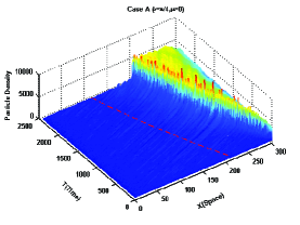
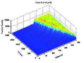
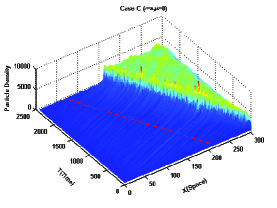
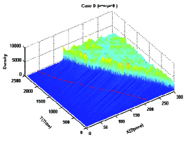
Figure 1: Four cases of density profiles for the entire simulation box vs the time. The dashed line represents the position of the FEB in each plot.

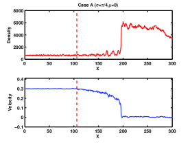
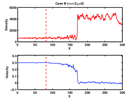
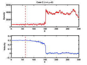
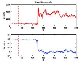
Figure 2: The velocity and density profiles (in the box frame) vs the position at the end of the simulation ($T_{max}$=2400) in the four cases. The vertical dashed line in each plot represents the position of the FEB, from case A to case D.

4.1 Shock Profiles

Figure 1 shows time sequences of the density profiles of four cases. In each plot, a shock forms and moves away from the reflective wall, and the dashed line represents the FEB position with the time in each case parallel to the shock front position. We can see that both the shock position and the FEB position are moving with a virtually constant velocity from the beginning of the simulation to the end of the simulation (i.e. $T_{max}$=2400) in each case. Simultaneously, as far as the positions of the FEB are concerned, we can see that the FEB position at the end of the simulation is significantly different in four different cases. As for the average density fluctuation in the downstream region, there are also apparent changes in different cases, and case A has the slowest shock propagation speed among these four cases. Case D has the lowest average density profile in the downstream region among these four cases. Because from Cases A to D the only difference is the prescribed scattering angular distribution, we conclude that these differences of the results for shock propagation speed and density profiles are decided by the standard deviation value $\sigma$ of the scattering angular distribution.

Figure 2 shows four cases of density and velocity profiles at the end of the simulations. From Cases A to D, the position of the FEB approaches zero as the value of the standard deviation $\sigma$ increases. The effects of the accelerated particles are clearly seen in the upstream smoothing of the velocity profiles in each case. In the simulations, when high-energy particles cross the shock front and diffuse upstream, they contribute negatively to the velocity profile. This reduces the grid-based velocity in the zones upstream of the shock, which in turn affects particles that are scattering in that region. In fact, the accelerated particles slow and heat the incoming flow and smooth the shock transition by their “back reaction.” As is obvious to see from the velocity and density plots, different scattering angular distributions produce different effects on the shock wave evolution. For the examples presented here, we consider that a difference of approximately 40.93% of the shock velocity is contributed by the scattering angle distribution.

4.2 Compression ratios

Here, we compare the compression ratios calculated from the velocity profiles with those from the density relationships. First, the value of the total compression ratio can simply be calculated from the formula

$$r_{u}=u_{1}/u_{2}$$ (9)

where $u_{1}=u_{0}+|v_{sh}|$ , $u_{2}=|v_{sh}|$, and $u_{1}(u_{2})$ is the upstream (downstream) velocity in the shock frame. The shock velocity at the end of the simulation ($T_{max}$) can be derived from the formula

$$v_{sh}=(X_{max}-X_{sh})/T_{max}$$ (10)

where $X_{max}$=300, $T_{max}$=2400, and $X_{sh}$ is the position of the shock at the end of the simulation (see Table 1). The specific calculated results are shown in Table 1.

But in terms of the specific shock structure as seen in Figure 3, an accurate subshock compression ratio calculation should be more complicated. In any one of the cases in Figure 3 (plotted in the box reference frame), we show the specific aspects of a shock modified by an energetic particle population whose mean-free-path is an increasing function of momentum. The shock structure in each plot consists of three main parts: precursor, subshock, and downstream. The smooth precursor is on the largest length scale between the FEB and near shock position $X_{sh}$, where the fluid speed gradually decreases from value $U_{0}$ to $v_{sub}$. The size of this precursor is almost the mean-free-path length of the maximum energy accelerated particles. One of the smallest scales is the subshock region with a sharp deflection of the fluid speed decreasing from $v_{sub}$ to $v_{box}=0$. The downstream region changes after the fluid speed becomes $v_{box}=0$ by microphysical dissipation processes. The gas subshock is just an ordinary discontinuous classical shock embedded in the comparably larger scale energetic particle shock (Berezhko & Ellison 1999). The value of $v_{sub}$ is determined by a sharp deflection of smooth curves in velocity profiles near the shock front, and the value of the subshock velocity increases from cases A, B, and C to Case D (i.e. $(v_{sub})_{A}<(v_{sub})_{B}<(v_{sub})_{C}<(v_{sub})_{D}$). All of the velocity profiles are based on the box frame. That value of the box frame’s velocity is zero ($v_{box}=0$) in all cases. The subshock compression ratio $r_{sub}$ is calculated from the formula $r_{sub}=(v_{sub}+|v_{sh}|)/|v_{sh}|$ . For the sake of the comparison of the values of $r_{sub}$ in different cases, the subshock compression ratios are calculated in the same shock frame reference, and the calculated results of $r_{sub}$ are shown in Table 1.

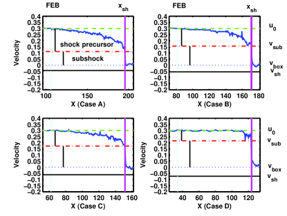
Figure 3: Velocity profiles in the shock region at the end of the simulation ($T_{max}$=2400) in the four cases; the vertical solid and dotted lines indicate the shock front and FEB in each plot, respectively; the horizontal solid, dotted, dot-dashed and dashed lines show the values of the shock velocity $v_{sh}$, velocity of box frame $v_{box}$, subshock velocity $v_{sub}$ and initial bulk velocity $U_{0}$, respectively. Two vertical bars in each plot represent the two deflections of velocity, the upper bar represents the part of the shock precursor and the lower one represents the subshock.

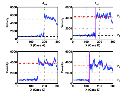
Figure 4: Density profiles in an entire simulation box at the end of the simulation ($T_{max}$=2400) in the four cases. The vertical solid line is located in the position of the shock front, the upper horizontal dot-dashed line represents the value of the downstream density $\rho_{2}$, and the lower horizontal dashed line indicates the value of the upstream density $\rho_{1}$ in each plot.

We then have the calculations of the compression ratio from the density relationships between the upstream and downstream flows:

$$r_{\rho}=\rho_{2}/\rho_{1}$$ (11)

where $\rho_{1}=n_{0}$ is the upstream density, and $\rho_{2}$ is the downstream density. This value is presented by which is the average value of $n_{k}$ over the downstream region.

$$\rho_{2}=\frac{1}{(k_{max}-k_{sh})}\displaystyle\sum_{k=k_{sh}}^{k_{max}}(n_{k})$$ (12)

where $n_{k}$ is the number density of particles in the “k” grid, $k_{sh}=x_{sh}/dx$ is the grid index of the shock at the end of the simulation ($T_{max}=2400$), and $k_{max}=600$ is the grid index of the $X_{max}$.

Figure 4 shows the complete density plots of the four cases at the end of the simulation. The value of the upstream density $\rho_{1}$ is the same constant value, which is equal to the initial density $n_{0}$ in each case. The value of the downstream density $\rho_{2}$ decreases from cases A, B, and C to Case D (i.e. $(\rho_{2})_{A}>(\rho_{2})_{B}>(\rho_{2})_{C}>(\rho_{2})_{D}$). Similarly, the detailed calculation results of the compression ratios $r_{\rho}$ are listed in Table 1. As listed in Table 1, the values of the subshock compression ratios, $r_{sub}$=2.5421, $r_{sub}$=3.0207, $r_{sub}$=3.3903, and $r_{sub}$=3.9444, corresponding to cases A, B, C, and D, respectively, are all lower than the standard value of $r=4$. Unfortunately, the values of total compression ratio $r_{u}$ and $r_{\rho}$ in each case are both higher than the standard value of $r=4$. But Knerr, Jokipii & Ellison (1996) consider that, if energy is lost from the system (e.g. by particles escaping via FEB), it is possible to produce a shock with a total compression ratio that is higher than the standard value predicted by the Rankine-Hugoniot (RH) conditions. We have examined the mass and energy losses via the FEB in each case. The results definitely show that the case with more energy losses would produce a higher total compression ratio than those in the case with less energy loss. Consequently, we consider that the energy loss rates would be affected by the prescribed scattering law. In any case, the energy losses are always an important and interesting problem in the nonlinear diffusive shock acceleration theory, so we will perform more precise research focusing on these problems in later papers. In addition, although the values of $r_{u}$ are correspondingly slightly higher than the value of $r_{\rho}$ in each case, all these differences are less than 3%, and the specific difference in each case is 2.9%,1.5%,1.3% and 0.18% corresponding to cases A, B, C and D. As seen from Figs. 3 and 4, the value of the total compression ratio $r_{tot}$, determined from the velocity profiles, is more consistent with the density profiles in each case (i.e. the total compression ratios $r_{tot}$ in all cases are satisfied by the Rankine-Hugoniot (RH) conditions : $u_{1}/u_{2}=\rho_{2}/\rho_{1}$). Therefore, it is not difficult for us to conclude that the total compression ratios $r_{u}$ and $r_{\rho}$ decrease as the value of the standard deviation $\sigma$ of the scattering angular distribution increases, but the subshock compression ratio $r_{sub}$ increases as the value of the standard deviation $\sigma$ of the scattering angular distribution increases.

4.3 Heating & acceleration

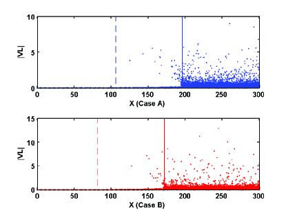
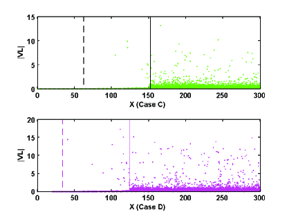
Figure 5: The scatter plots of the particle’s thermal velocities in the local frame vs its position at the end of the simulations ($T_{max}$=2400), and the vertical dashed line and solid line in each plot indicate the approximate position of the FEB and shock front, respectively. Only the ratio of 1/12 of the total number of particles are plotted.

Here we contrast between two important aspects of the heating and acceleration processes in the diffusive shock acceleration. Figure 5 shows the particles’ scatter plots in four cases at the end of the simulations ($T_{max}$=2400). In each case, particles with local velocity scatter into the simulation box’s position. A large amount of particles that do not get injected into the Fermi acceleration mechanism and that have lower thermal velocities stay in the downstream region, and a few particles with higher energy via multiple shock encounters can move far away from the shock front and even escape from the FEB. From Cases A to D, more and more particles are injected into the Fermi acceleration mechanism, and they gain greater and greater maximum energy. Obviously, the maximum thermal velocity in Case D would be several times that of the ones in Case A. We supposed that this difference is mainly contributed by the scattering angular distribution function $f(\delta\theta,\delta\phi)$. In short, the majority of particles, which flow toward the shock, cross the shock only once, and (after scattering) remain fairly stationary in the downstream region, which would consist of the “heated” elements, and a few high-energy particles represent the “power-law” part of the simulated particles flows. Actually, the “back pressure” from the accelerated particles via their back reaction reduces the incoming fluid speed, leading to a smoothed precursor heating. Therefore, an anisotropic scattering angular distribution in the shocks dominate the “gas heating” process in the simulated plasma, and isotropic scattering angular distribution in the shocks play an important role in nonlinear acceleration of the energetic particles via the Fermi mechanism, and they dominate the “precursor heating”.

4.4 Energy spectra

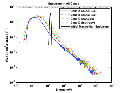
Figure 6: The final energy spectrum in the four cases and the initial energy spectrum plots. The thick solid line with a narrow peak at $E_{0}=$1.3105keV represents the initial Maxwell energy distribution. The solid, dashed, dot-dashed, and dotted extended curves indicate the simulated particles’ energy spectral distribution, averaged over the entire downstream region, at the end of the simulations ($T_{max}$=2400), corresponding to Cases A, B, C, and D, respectively. Most particles cross the shock only once, producing the large broad peak centered at E${}_{A}\sim$ 0.05keV, E${}_{B}\sim$0. 1keV, E${}_{C}\sim$ 0.15keV, and E${}_{D}\sim$0.20keV in Cases A, B, C, and D, respectively. However, some particles gain enough energy via the Fermi acceleration mechanism to produce the “power-law” tail in the energy spectrum with the cutoff at $E_{A}$=1.10 MeV, $E_{B}$=2.41 MeV, $E_{C}$=2.98 MeV, and $E_{D}$=4.01 MeV corresponding to Cases A, B, C, and D. All these energy spectra are plotted in the same shock frame.

Spectra calculated in the shock frame from the initial and final particle (proton) energy distributions in all cases are shown in Figure 6. The energy units in this plot are derived from the scaling parameters presented in Table 2 (see Appendix A). Initially, all particles move toward the wall with a certain thermal spread in energy. A narrow peak at E=1.3105keV represents the initial Maxwell energy distribution. The four extended curves indicate the simulated particle energy spectral distribution, averaged over the entire downstream region, at the end of the simulations, corresponding to the four cases, respectively. The majority of the particles cross the shock only once, producing an expanded energy spectrum with a central peak at E${}_{A}\sim$ 0.05keV, E${}_{B}\sim$0.1keV, E${}_{C}\sim$ 0.15keV, and E${}_{D}\sim$0.20keV in Cases A, B, C, and D, respectively. However, as is shown in Figure 6, the minority of the particles gain enough energy via the Fermi acceleration mechanism to produce the “power-law” tail in the energy spectrum with the cutoff at $E_{A}$=1.10 MeV, $E_{B}$=2.41 MeV, $E_{C}$=2.98 MeV and $E_{D}$=4.01 MeV corresponding to Cases A, B, C and D, respectively. For more details about the calculated results, see Table 1. It is evident from Figure 6 that the values of the central peak of the extended energy spectra in the four cases are far from the initial energy peak in their respective order. This means the values of the central peak in each case increase as the value of the standard deviation of the scattering angular distribution increases, and each extended curve shows a harder power-law slope in its high-energy tail as the expand energy range increases, respectively. Therefore, we can see that the case of applying an anisotropic scattering angular distribution function will produce a slightly softer energy spectrum, and the case of applying an isotropic scattering angular distribution will produce a slightly harder energy spectrum.

4.5 Spectral index & compression ratios

Usually, we could predict the power-law energy spectral index from diffusive shock acceleration theory:

$$dJ/dE\propto E^{-\Gamma}$$ (13)

where $dJ/dE$ is the energy flux and $\Gamma$ is the energy spectral index, and

$$\Gamma=(r+2)/(2\times(r-1)).$$ (14)

According to Equation 14, we substituted the values of the compression ratio $r$ with two group values of $r_{tot}$ and $r_{sub}$ obtained in each case. Then, the two group energy spectral indices $\Gamma_{tot}$ and $\Gamma_{sub}$ in each case are calculated. Two groups’ spectral index values are listed in Table 1 as $\Gamma_{A}$= 0.7167, $\Gamma_{B}$ =0.7677, $\Gamma_{C}$ =0.8083, and $\Gamma_{D}$=0.8667 in the total group $\Gamma_{tot}$, and $\Gamma_{A}$= 1.4727, $\Gamma_{B}$ =1.2423, $\Gamma_{C}$ =1.1275, and $\Gamma_{D}$=1.0094 in subshock group $\Gamma_{sub}$, corresponding to the cases A, B, C, and D, respectively. As shown in Figure 7, from Cases A to D, all of the values of the subshock’s energy spectral index $\Gamma_{sub}>1$ and show that a slightly harder power-law slope in the respective order. From Cases A to D, all of the values of the total energy spectral index $\Gamma_{tot}<1$ show a slightly decreasingly deviation from the power-law slope in the respective energy spectrum.

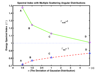
Figure 7: The correlation of the deviation value of the Gaussian distribution vs the energy spectral index. The triangles represent the total energy spectral index in each case. The circles indicate the subshock’s energy spectral index in each case. From Cases A to D, all of the values of the subshock’s energy spectral index $\Gamma_{sub}>1$ show a slightly harder power-law slope in the respective order. From Cases A to D, all of the values of the total energy spectral index $\Gamma_{tot}<1$ show a slightly decreasing deviation from the power-law slope in the respective energy spectrum.

5 Summary and conclusions

We followed the previous dynamical Monte Carlo simulation by using a new code based on the Matlab platform independently, and presented the same results as the outcome from the previous simulation. In addition, we successfully extended the simulation include the multiple scattering angular distributions using these new codes to study the diffusive shock acceleration mechanism further.

In conclusion, the comparison of the calculated results come from different extensive cases, we find that the total energy spectral index increases as the standard deviation value of the scattering angular distribution increases, but the subshock’s energy spectral index decreases as the standard deviation value of the scattering angular distribution increases. In these multiple scattering angular distribution simulation cases, the prescribed scattering law dominates the shock structure and plays an important role in balancing whether the particles have more heating or more acceleration. In other words, the cases with anisotropic scattering distribution give the overall velocity-deflection precursor sizes, which are larger than the isotropic case, and give a relatively greater “heating” effect or less “acceleration” effect on background flows than does the isotropic case.

As a result, the shock compression ratio and the energy spectral index are both modified naturally by the prescribed scattering law. Specifically, the cases of applying an anisotropic scattering distribution function will produce a slightly softer subshock’s energy spectral index, and the case of applying an isotropic scattering angular distribution will produce a slightly harder subshock’s energy spectral index. Simultaneously, from the isotropic case to the anisotropic case, the total energy spectrum shows an increasing deviation from the “power-law” distribution.

In addition, although we find no case producing the total compression ratio which should be less than the standard value 4 according to the Rankine-Hugoniot (RH) jump conditions, the fact is clear that the prescribed scattering angular distribution function would have an effect on the total compression ratio. If there is a suitably prescribed scattering law that leads to much less energy loss, it is possible to constrain the total compression ratio to be less than 4.

Appendix A Simulation box & parameters

With respect to the validity and consistency of verifying the previous dynamic Monte Carlo simulation method, the present simulation program uses the same simulation box and identical parameters as the previous dynamical Monte Carlo simulation (Knerr, Jokipii & Ellison 1996). The schematic diagram of the simulation box is shown in Figure 8 and all the simulation parameters are listed in Table 2.

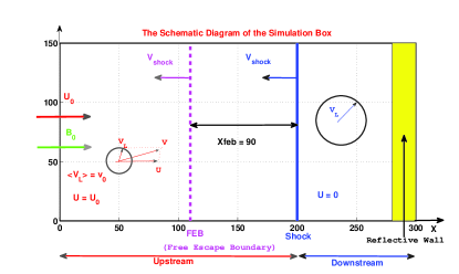
Figure 8: Shock is produced by supersonic flow toward the stationary reflective wall to the right. Continuous inflow of new particles occurs at the left boundary. Inflow velocity is $U_{0}$, a particle’s total velocity is $V$, the local frame particle velocity is $V_{L}$, and thermal velocity $<V_{L}>=v_{0}$. The two circles represent one typical particle in the upstream region and one in the downstream region, respectively. The vertical solid line represents the shock front, the vertical dashed line represents the FEB, the velocity of the shock is $V_{shock}$, size of the foreshock region is $Xfeb=90$, the upstream flow velocity $U=U_{0}$, and the downstream flow velocity is $U=0$. The magnetic field $B_{0}$ and inflow velocity $U_{0}$ are both normal to the shock front (see Knerr, Jokipii & Ellison 1996).

Table 2: The parameters of the simulated cases

Inflow velocity	$u_{0}$=0. 3	403km/s
Thermal speed	$\upsilon_{0}$=0. 02	26. 9km/s
Scattering time	$\tau$=0. 833	0. 13s
Box size	$X_{max}$=300	$10R_{e}$
Total time	$T_{max}$=2400	6. 3minutes
Time step size	$dt$=1/30	0. 0053s
Number of zones	$nx$=600	. . .
Initial particles per cell	$n_{0}$=650	. . .
FEB distance	$X_{feb}$=90	$3R_{e}$