Ultimate quantum bounds on mass measurements with a nano-mechanical resonator

Abstract

I establish the fundamental lower bound on the mass that can be measured with a nano-mechanical resonator in a given quantum state based on the fundamental quantum Cramér–Rao bound, and identify the quantum states which will allow the largest sensitivity for a given maximum energy. I show that with existing carbon nanotube resonators it should be possible in principle to measure a thousandth of the mass of an electron, and future improvements might allow to reach a regime where one can measure the relativistic change of mass due to absorption of a single photon, or the creation of a chemical bond.

1 Introduction

High-quality nano-mechanical resonators can act as extremely sensitive sensors of adsorbed material. Impressive progress has been made in this direction over the last few years: In 2004, experiments reached a level of sensitivity of femto-grams [1], atto-grams [2], and two years later already zepto-grams [3]. Gas chromatography at the single molecular level was achieved a year ago [4], and brought a vast range of chemical and biological applications in reach. A mass sensitivity as small as half a gold atom has been demonstrated using a nano-mechanical resonator based on a carbon nano-tube [5]. At the same time, large efforts have been spent to cool down a nano-mechanical resonator to its ground state, with the ultimate goal of engineering arbitrary quantum states (see e.g. [6, 7, 8, 9, 10]). The ground state was reached very recently for a piezo-electrical device [11]. It is therefore natural to ask whether the sensitivity of mass measurements could be increased further by engineering the quantum state of a nano-mechanical resonator, and what would be the truly fundamental lower bound on the mass that can be measured based only on the laws of quantum mechanics. Early on, theoretical investigations tried to find the limitations of mass measurements with a nano-mechanical resonator [12, 13, 14]. But the bounds which were derived so far assume that one measures the linear response of the resonator driven at its resonance frequency [12, 13, 15, 14]. In the experiments, a variety of different read-out and/or cooling techniques (e.g. optical [16, 17, 18, 19, 20, 21, 22], through electrostatic effects [23, 2, 24, 25], mechanical [26], or even field emission in the case of a nano-tube [27]) were used. Most of these do use linear transduction, but whether this is the optimal measurement procedure is an open question.

The truly fundamental lowest (but achievable) bound on the mass sensitivity is a function of the quantum state of the resonator, and optimized over all possible measurement procedures. It will be calculated below using quantum parameter estimation theory, which leads to the ultimate limit of sensitivity, the quantum Cramér-Rao bound [28]. It becomes relevant once all other limitations such as technical noise, adsorption-desorption noise, momentum exchange noise, etc. have been eliminated [15]. I will even assume a harmonic oscillator without any dissipation (and thus decoherence effects), as mixed states can only decrease the ultimate sensitivity compared to the pure states from which they are mixed [29]. Nevertheless, the bounds I calculate are attainable in principle if the idealized conditions are met, and therefore set an important benchmark to which the performance of existing sensors should be compared to. As a guide to further improving the sensitivity of mass-sensing using quantum-engineered states of a nano-oscillator, I determine the optimal quantum state for a given maximum number of excitation quanta in the oscillator.

2 Quantum parameter estimation theory

For small enough excitation amplitudes, the nano-mechanical resonator can be modelled as a harmonic oscillator with mass $M$ and effective spring constant $D$ [5], resonance frequency $\omega=\sqrt{D/M}$, and hamiltonian $H_{\omega}=\hbar\omega(a^{\dagger}_{\omega}a_{\omega}+\frac{1}{2})$ with the usual raising (lowering) operators $a^{\dagger}_{\omega}$ ($a_{\omega}$). If a small mass $\delta M$ is added to the oscillator, its frequency changes to $\tilde{\omega}=\omega(1-\epsilon)$ with $\epsilon=(1/2)\delta M/M$, and we obtain the new hamiltonian $H_{\tilde{\omega}}$ from $H_{\omega}$ by replacing $\omega\to\tilde{\omega}$ everywhere. An arbitrary initial quantum state $\rho_{0}$ is thus propagated to $\rho(\omega,t)=U(\omega,t)\rho_{0}U^{\dagger}(\omega,t)$ (or $\rho(\tilde{\omega},t)$, respectively), if no mass (or the mass $\delta M$) is adsorbed at $t=0$, where $U(\omega,t)=\exp(-{\rm i}H_{\omega}t/\hbar)$. Note that this assumes that the energy of the oscillator is conserved in the adsorption process, i.e. the additional mass is deposited with zero differential speed onto the oscillator. The distinguishability of the two states $\rho(\omega,t)$ and $\rho(\tilde{\omega},t)$ determines the smallest $\delta M$ that can be measured. In general, for any density matrix $\rho(x)$ that depends on some parameter $x$, the smallest $\delta x$ that can be resolved from $N$ measurements of an observable $A$ (starting always from an identically prepared state) is given by [28]

$$\delta x=\frac{\langle\delta A^{2}\rangle_{x}^{1/2}}{\sqrt{N}|\frac{\partial}{\partial x}\langle A\rangle_{x}|}\,.$$ (1)

It has the interpretation of the uncertainty of $A$ in state $\rho(x)$ as judged by $N$ measurements, renormalized by the “speed” by which the mean value of $A$ changes as function of $x$. In other words, $x$ has to change by an amount that moves the average value of $A$ by at least its uncertainty. Optimizing over all possible measurements leads to the quantum Cramér-Rao bound [28],

$$\delta x\geq\delta x_{\rm min}\equiv\frac{1}{2\sqrt{N}\frac{d_{\rm Bures}(\rho(x),\rho(x+dx))}{dx}}\,,$$ (2)

where $d_{\rm Bures}(\rho(x),\rho(x+dx))$ is the Bures distance between $\rho(x)$ and $\rho(x+dx)$ (also called Fisher information), defined as $d_{\rm Bures}(\rho_{1},\rho_{2})=\sqrt{2}\sqrt{1-\sqrt{F(\rho_{1},\rho_{2})}}$ through the fidelity $\sqrt{F(\rho_{1},\rho_{2})}=\mathrm{tr}((\rho_{1}^{1/2}\rho_{2}\rho_{1}^{1/2})^{1/2})$. Thus, in our case, we obtain the minimal measurable mass $\delta M_{\rm min}$ by evaluating the Bures distance between $\rho(\omega,t)$ and $\rho(\tilde{\omega},t)$ in the limit $\epsilon\to 0$. It is important to note that (2) is, in the limit of large $N$, an achievable lower bound [28]. It does take into account effects such as back-action and the quantum noise of the system.

3 Pure states

In the case of two pure states, we have simply $F(|\psi\rangle\langle\psi|,|\phi\rangle\langle\phi|)^{1/2}=|\langle\psi|\phi\rangle|$. Starting from an initial state $|\psi(0)\rangle=\sum_{n=0}^{\infty}c_{n}|n\rangle_{\omega}$, we have the overlap at time $t$,

$$\langle\psi(t)|\tilde{\psi}(t)\rangle = \sum_{n,m,k}c_{n}^{*}c_{k}{\rm e}^{-i(\tilde{E}_{m}-E_{n})t/\hbar}$$ (3)

$$\times R_{\tilde{\omega}\omega}(m,k)R_{\tilde{\omega}\omega}(m,n)\,,$$

where $R_{\tilde{\omega}\omega}(m,n)={{}_{\tilde{\omega}}}\langle m|n\rangle_{\omega}=R_{\omega\tilde{\omega}}(n,m)$ denotes the overlap matrix element between energy eigenstates of the two oscillators with frequency $\tilde{\omega}$ and $\omega$, and the coefficients $c_{n}^{*}$, $c_{k}$ are expressed in the energy eigenbasis of the unperturbed oscillator. They are [30]

$$R_{\tilde{\omega}\omega}(m,n) = (2^{-(m+n)}qm!n!)^{1/2}$$

$$\times\sum_{r=0,1}^{[m,n]}\frac{(2q)^{r}}{r!}\frac{y^{(m+n-2r)/2}(-1)^{(m-r)/2}}{(\frac{1}{2}(n-r))!(\frac{1}{2}(m-r))!}\,,$$

if $m,n$ are both even or both odd (otherwise $R_{\tilde{\omega}\omega}(m,n)=0$), and $[m,n]$ denotes the smaller of the two integers $m,n$. The sum over $r$ runs over even (odd) integers for $[m,n]$ even (odd), respectively, and $y=(\omega-\tilde{\omega})/(\omega+\tilde{\omega})$, $q=2(\omega\tilde{\omega})^{1/2}/(\omega+\tilde{\omega})$. We need $|\langle\psi(t)|\tilde{\psi}(t)\rangle|$ to second order in $\epsilon$. We find $F=1+\epsilon^{2}f(\{c_{m}\},t)$ with

$$f(\{c_{m}\},t) = \Big{[}\sum_{m=0}^{\infty}\big{\{}\frac{1}{2}\sqrt{(m+1)(m+2)}$$

$$\times \Im(c_{m}c_{m+2}^{*}({\rm e}^{2{\rm i}\tau}-1))+\tau m|c_{m}|^{2}\big{\}}\Big{]}^{2}$$

$$- \sum_{m=0}^{\infty}\Big{\{}\left(\frac{(m^{2}+m+1)\sin^{2}\tau}{2}+m^{2}\tau^{2}\right)|c_{m}|^{2}$$

$$- \sqrt{(m+1)^{3}(m+2)}\tau\,\Im((1-{\rm e}^{2{\rm i}\tau})c_{m+2}^{*}c_{m})$$

$$- \frac{1}{8}\sqrt{(m+1)(m+2)(m+3)(m+4)}$$

$$\times \Re((1-{\rm e}^{2{\rm i}\tau})^{2}c_{m}c_{m+4}^{*})\Big{\}}\,$$

and $\tau=\omega t$. Inserting $F$ in $d_{\rm Bures}$, we find immediately $d_{\rm Bures}(|\psi(t)\rangle\langle\psi(t)|,|\tilde{\psi}(t)\rangle\langle\tilde{\psi}(t)|)=\epsilon|f(\{c_{m}\},t)|^{1/2}$, and thus

$$\frac{\delta M_{\rm min}}{M}=\frac{1}{\sqrt{N}|f(\{c_{m}\},t)|^{1/2}}\,.$$ (6)

Eq.(6) together with (3) constitutes the central result of this report which we now explore for particular cases.

3.1 Fock state

For $|\psi(0)\rangle=|n\rangle$, we have $f=-(1/2)(n^{2}+n+1)\sin^{2}\tau\equiv f_{n}^{\rm Fock}$ for all $n\geq 0$. The largest absolute value is achieved for $\tau=\pi/2(\mod 2\pi)$, and leads to

$$\frac{\delta M_{\rm min}}{M}=\sqrt{\frac{2}{N}}\frac{1}{\sqrt{n^{2}+n+1}}\sim\sqrt{\frac{2}{N}}\frac{1}{n}\mbox{ for }n\gg 1\,.$$ (7)

Thus, one can measure, at least in principle, arbitrarily small masses within the same fixed time interval by increasing the excitation of the harmonic oscillator. In reality, of course, non-harmonicities will start to arise at some level of excitation and the present analysis will then have to be extended to a more complicated hamiltonian [31]. The ground state $n=0$ of the harmonic oscillator allows to measure a mass which, for a single readout, can be of the order of the mass of the oscillator itself, $\delta M/M\geq\sqrt{2/N}/|\sin\tau|$. Increasing $\tau$ does not help beyond $\tau=\pi/2$, as $f_{n}^{\rm Fock}$ is periodic in $\tau$.

3.2 Little Schrödinger cat states

Given that (3) depends on coherences between states $|n\rangle$, $|n+2\rangle$, and $|n+4\rangle$, one might wonder whether the precision could be increased further by using superpositions of these states. The state $|\psi(0)\rangle=(|n\rangle+|n+2\rangle)/\sqrt{2}\equiv|\psi_{S1}\rangle$ leads to

$$f=\frac{1}{16}\big{(}(n+1)(n+2)\sin^{2}(2\tau)-8(n^{2}+3n+4)\sin^{2}\tau\big{)}-\tau^{2}\,.$$ (8)

The maximum of the periodic term is again achieved for $\tau=\pi/2\,(\mod 2\pi)$. For fixed $\tau\neq k\pi$ ($k\in\mathbb{N}$) and $n\gg\tau$, this term dominates and leads to $\delta M_{\rm min}/M\simeq\sqrt{2/N}/n$, just as for the Fock state. However, for fixed $n$, we can get an arbitrarily small $\delta M/M$ by increasing $\tau$, as the last term in (8) leads to $\delta M_{\rm min}/M\simeq\sqrt{2/N}/\tau$ for $\tau\gg n$. Note that this improvement is beyond the usual factor $1/\sqrt{t}$ from increasing the measurement time. Indeed, the sensitivity $\delta M\sqrt{t}$ in (g/$\sqrt{\mbox{Hz}}$) still improves as $\propto 1/\sqrt{t}$.

The state $|\psi(0)\rangle=(|n\rangle+|n+4\rangle)/\sqrt{2}\equiv|\psi_{S2}\rangle$ gives

$$f = -\frac{1}{4}\Big{(}2(n^{2}+5n+11)\sin^{2}\tau$$

$$+\sqrt{(n+1)(n+2)(n+3)(n+4)}\cos(2\tau)\sin^{2}\tau\Big{)}$$

$$-4\tau^{2}\,.$$

The maximum of the periodic terms (relevant for fixed $\tau$ and $n\gg\tau\gtrsim 1$) is close to $\tau=\pi/3$ with $|f|\simeq 9n^{2}/32$, which gives a $\delta M_{\rm min}$ 33% larger than for a Fock state with $n$ excitations. For fixed $n$ and $\tau\gg n$, the factor 4 in front of $\tau^{2}$ in (3.2) reduces $\delta M_{\rm min}/M$ by a factor 2 compared to $|\psi_{S1}\rangle$.

3.3 Coherent state

For a coherent state $|\alpha\rangle=\exp(-|\alpha|^{2}/2)\sum_{n=0}^{\infty}(\alpha^{n}/\sqrt{n!})|n\rangle$, and $\alpha\in\mathbb{R}$, we have

$$f=-\left(\frac{1}{2}+\alpha^{2}\right)\sin^{2}\tau-\alpha^{2}\tau\left(\tau+\sin(2\tau)\right)\,.\,\,\,\,\,\,(10)$$

For fixed $\tau\gg 1$ and $\alpha^{2}\gg 1$, we find $f\simeq-\alpha^{2}\tau^{2}$, and hence $\delta M_{\rm min}/M\simeq 1/(\sqrt{N}\alpha\tau)=1/(\sqrt{N\langle n\rangle}\tau)$. Thus, for a coherent state, the sensitivity scales as the inverse square root of the (average) number of excitations in the oscillator, and one can, at least in principle, resolve arbitrarily small masses. We see again that $\delta M_{\rm min}$ reduces faster than $1/\sqrt{t}$ with measurement time. Compared to a Fock state with $n=\alpha^{2}$, there is a factor $\sqrt{\langle n\rangle/2}$ penalty in the scaling with $\langle n\rangle$ (but one gains a factor $1/\tau$). For $\alpha=0$ we find $f=-\sin^{2}\tau/2$ which leads back to the result for the Fock state $n=0$. “

3.4 Optimal state

What is the best sensitivity that can be achieved for a given maximum number $L$ of excitations and fixed measurement time? From (3) we see that for $\tau\gg 1$, the terms quadratic in $t$ dominate and give simply $|f|=\tau^{2}(\langle n^{2}\rangle-\langle n\rangle^{2})$. Hence, in this case the optimal pure state is the one which maximizes the excitation number fluctuations. One easily shows that this state has the form of an “ON” state (half a “NOON” state [32]), $|\psi_{\rm ON}\rangle=(|0\rangle+{\rm e}^{{\rm i}\varphi}|L\rangle)/\sqrt{2}$, where $\varphi$ is an irrelevant phase which we will choose equal zero. It leads to $|f_{\rm ON}|\equiv|f(\psi_{\rm ON},\tau)|\simeq\tau^{2}L^{2}/4$, and thus a minimal mass $\delta M_{\rm min}/M=2/(\sqrt{N}\tau L)$. Fig.1 shows a comparison of the (inverse) minimal mass for $\psi_{\rm ON}$ with the true minimal mass for given $\tau$ and the same $L$, obtained by numerically maximizing $|f|$, for $L=3$. We see that $|f_{\rm ON}|$ approximates the best possible $|f|$ very well, even for $\tau\sim 1$. For $\tau=k\pi$, $k\in\mathbb{N}$, $|f_{\rm ON}|$ gives in fact the exact result, as is obvious from (3). Fig.1 also shows the result for a coherent state with the same average number of excitations as the ON state, $\langle n\rangle=3/2$. It leads for small $\tau$ to comparable sensitivity as the optimal state with $L=3$. At $\tau=\pi/2$, the optimal pure state with $L=3$ allows still a reduction of $\delta M_{\rm min}/M$ by $\sim 4$% compared to $\psi_{\rm ON}$, and by $\sim 18$% compared to the Fock state with the same $L$.

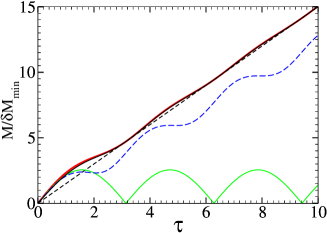
Figure 1: Inverse minimal measurable mass $M/\delta M_{\rm min}$ (for $N=1$) as function of $\tau$ for selected pure states. Green line: Fock state $|n=3\rangle$; Full black line: ON state $|\psi_{\rm ON}\rangle=(|0\rangle+|3\rangle)/\sqrt{2}$; Dashed black line: asymptotic behavior $3\tau/2$ for $|\psi_{\rm ON}\rangle$; Red line: optimal state with at most $L=3$ quanta in the oscillator; Dashed blue line: Coherent state with the same average number of excitations as the ON state ($\langle n\rangle=3/2$).

Fig.2 shows the Wigner function, defined for a pure state $|\psi\rangle$ by [33]

$$W(x,p)=\frac{1}{\pi}\int_{-\infty}^{\infty}dy\psi^{*}(x-y)\psi(x+y){\rm e}^{-2{\rm i}yp}\,,$$ (10)

(with all lengths in units of the oscillator length $x_{0}=\hbar^{1/2}/(DM)^{1/4}$ and $p$ in units of $\hbar/x_{0}$), for the optimal state for $L=4$ and $\tau=\pi/2$, $|\psi_{\rm opt}\rangle\simeq(-0.62057+0.0305{\rm i})|0\rangle-(0.00059+0.01198{\rm i})|2\rangle+(0.78252-0.038852{\rm i})|4\rangle$. $|\psi_{\rm ON}\rangle$ and $|\psi_{\rm opt}\rangle$ have very similar Wigner functions, characterized by four lobes in azimuthal direction which guarantee minimal phase uncertainty, as is to be expected from the requirement of minimal noise and maximum uncertainty in the number of excitations. Rotations of $|\psi_{\rm opt}\rangle$ through evolution with the unperturbed hamiltonian before the adsorption of mass clearly leave $\delta M_{\rm min}$ invariant.

Figure 2: Wigner function of the optimal initial state for $L=4$, $\tau=\pi/2$

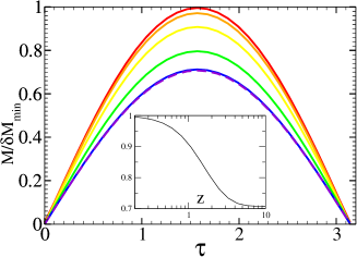
Figure 3: Inverse minimal measurable mass $M/\delta M_{\rm min}$ in a thermal state as function of dimensionless time $\tau=\omega t$ for inverse dimensionless temperatures $z=\hbar\omega/(k_{B}T)=0.2,0.5,1.0,2.0,5.0$ and 10.0 (red, orange, yellow, green, blue, and dashed purple line, respectively). Inset: $M/\delta M_{\rm min}$ as function of $z$ for $\tau=\pi/2$.

It is an open question how to experimentally realize the optimal state. In [11], non-trivial quantum states were obtained by coupling the harmonic oscillator to a super-conducting qubit whose quantum state can be readily manipulated. Other schemes for engineering the quantum state of a nano-mechanical harmonic oscillator were proposed in [34].

Among the pure states considered, the coherent states certainly come closest to the typical experimental situation, where the oscillator is cooled to low temperature and driven on resonance. Inserting typical numbers for micromachined resonators, $M=10^{-16}$g [14], $\omega=$1GHz, an evolution time $\tau=10^{6}$, and an excitation with $\langle n\rangle\sim 10^{10}$ quanta (driving energy $E_{d}=10^{-15}$J in [14]), we find $\delta M_{\rm min}\simeq 10^{-27}{\rm g}/\sqrt{N}$, or roughly the mass of an electron for a single readout, $N=1$. Higher masses (e.g. $M\sim 10^{-14}g$ in [3]) give proportionally higher $\delta M_{\rm min}$, everything else equal. In assuming $\tau=10^{6}$, we have made a pessimistic estimate in the sense of using the shortest sensing time allowed by the inverse bandwidth 1 kHz. Measuring during longer times decreases $\delta M_{\rm min}$ further. On the other hand, $\tau$ might be limited by decoherence and dissipation, such that for later times another (mixed) quantum state becomes relevant. These effects are, at least in principle, avoidable, and in such a highly idealized situation (which is, however, relevant as utlimate achievable goal), $\tau$ in eq.(3) is given by the measurement time. The mass $\delta M_{\rm min}\simeq 10^{-27}{\rm g}$ agrees with the prediction of [14], but the agreement appears to be a coincidence: The result in [14], based purely on noise considerations, still decreases as $1/\sqrt{Q}$ with the quality $Q$ of the resonator, whereas (3.3) is independent of $Q$, taken as infinity in the present analysis. Also, while in the regime $\tau\gg\alpha$ relevant for the above numbers ($\alpha=10^{5}$) both $\delta M_{\rm min}/M$ and the result in [14] scale as $1/\sqrt{\langle n\rangle}$, [14] predicts a proportionality to $1/\sqrt{\tau}$ if one identifies the inverse bandwidth $1/\Delta f$ with $t$, instead of the $1/\tau$ behavior that follows from (3.3).

Carbon nanotube resonators have typically much smaller masses than micro-engineered ones (of order $M\simeq 10^{-18}$g [5]) with comparable resonance frequency ($\omega=2\pi\times 328.5$MHz in [5]), and can therefore resolve in principle even smaller masses. Assuming a coherent state with oscillation amplitude of about 10nm for the carbon nanotube resonator in [5] and a sampling time of 100ms, $\delta M_{\rm min}$ according to (3.3) is of the order of a thousandth of an electron mass.

4 Mixed states

In general, due to the joint-convexity of the Bures distance, mixed states do not allow better sensitivities than the pure states from which they are mixed, as long as the weights are independent of the parameter to be measured and the evolution is linear in the state [29]. Evaluating the Bures distance between two mixed states is much more difficult than for pure states. Nevertheless, one can evaluate the Bures distance numerically. One may also obtain an upper bound on $d_{\rm Bures}$ using the joint-convexity of $d_{\rm Bures}$, which leads to a (typically non-achievable) lower bound on $\delta M_{\rm min}$. An achievable upper bound on $\delta M_{\rm min}$ can be found by considering a particular measurement $A$ in (1).

As an example, consider the thermal state $\rho=\sum_{n=0}^{\infty}p_{n}|n\rangle\langle n|$, with $p_{n}={\rm e}^{-nz}(1-{\rm e}^{-z})$, $z=\beta\hbar\omega$, $\beta=1/k_{B}T$ the inverse temperature, and $k_{B}$ the Boltzmann constant. Using the invariance of the thermal state under the time evolution governed by $H_{\omega}$ and the joint convexity of $d_{\rm Bures}(\rho_{1},\rho_{2})$, one shows easily that $d_{\rm Bures}/dx\leq\sum_{n}p_{n}|f_{n}^{\rm Fock}|^{1/2}\leq|\sin\tau|/(\sqrt{2}(1-\exp(-z))$. For $z\to\infty$, this bound coincides with the exact result for the groundstate $n=0$. We may choose a measurement of the width $A=x^{2}$ as a way of measuring the change of mass. Thermal average $\langle x^{2}\rangle=(\hbar/(2\sqrt{DM}))\coth(z/2)$ and fluctuations $\langle\delta(x^{2})\rangle=(\langle x^{4}\rangle-\langle x^{2}\rangle^{2})^{1/2}=(\hbar/\sqrt{2DM})\coth(z/2)$ give an achievable upper bound $\delta M_{\rm min}/M\leq 2\sqrt{2/N}\sinh z/(\sinh z-z)$. For $z\to\infty$ this bound is only a factor 2 above the best possible value for the groundstate $n=0$, whereas for $z\to 0$ the bound diverges. Fig.3 shows the exact $M/\delta M_{\rm min}$ obtained by evaluating the Bures distance numerically. We see that $\delta M_{\rm min}/M$ is periodic in $\tau$, just as for the ground state. Increasing the temperature helps, as higher Fock states start to contribute, but at most a factor $\sqrt{2}$ can be gained, and $\delta M_{\rm min}$ remains bounded by the mass of the oscillator itself for all temperatures.

5 Conclusions

In summary, I have calculated the smallest measurable adsorbed mass $\delta M_{\rm min}$ on a nano-mechanical harmonic resonator in an arbitrary pure state, based on the fundamental quantum Cramér-Rao bound. The analysis shows that a coherent state allows to achieve a $\delta M_{\rm min}/M$ that scales for fixed measurement time as the inverse square root of the average number of excitations. For a given maximum number $n$ of excitations, I found the optimal quantum state, which for large $\tau$ is $|\psi_{\rm ON}\rangle=(|0\rangle+|n\rangle)/\sqrt{2}$, with a sensitivity that scales as $1/n$. For $\tau\neq k\pi$, $k\in\mathbb{N}$, the sensitivity can be further enhanced. Even with a coherent state of a carbon nanotube resonator [5], the smallest resolvable mass should be of the order of a thousandth of an electron mass. If two more orders of magnitude could be gained (say by increasing $\tau$ and the number of excitations), the regime could be reached where one can weigh the relativistic mass change due to the formation of a chemical bond or the absorption of a photon (energies of order 1 eV).

References

- [1] \NameLavrik N. V., Sepaniak M. J. Datskos P. G. \REVIEWReview of Scientific Instruments 7520042229.
- [2] \NameIlic B. \REVIEWJournal of Applied Physics 9520043694.
- [3] \NameYang Y. T., Callegari C., Feng X. L., Ekinci K. L. Roukes M. L. \REVIEWNano Letters 62006583.
- [4] \NameNaik A. K., Hanay M. S., Hiebert W. K., Feng X. L. Roukes M. L. \REVIEWNature Nanotechnology 42009445.
- [5] \NameJensen K., Kim K. Zettl A. \REVIEWNature Nanotechnology 32008533.
- [6] \NameMartin I., Shnirman A., Tian L. Zoller P. \REVIEWPhysical Review B 692004125339.
- [7] \NameRocheleau T., Ndukum T., Macklin C., Hertzberg J. B., Clerk A. A. Schwab K. C. \REVIEWNature 463201072.
- [8] \NameBuks E., Segev E., Zaitsev S., Abdo B. Blencowe M. P. \REVIEWEurophysics Letters (EPL) 81200810001.
- [9] \NameMarquardt F. Girvin S. M. \REVIEWPhysics 2200940.
- [10] \NameKippenberg T. J. Vahala K. J. \REVIEWScience 32120081172.
- [11] \NameO’Connell A. D., Hofheinz M., Ansmann M., Bialczak R. C., Lenander M., Lucero E., Neeley M., Sank D., Wang H., Weides M., Wenner J., Martinis J. M. Cleland A. N. \REVIEWNature 4642010697.
- [12] \NameCleland A. N. Roukes M. L. \REVIEWJournal of Applied Physics 9220022758.
- [13] \NameClerk A. \REVIEWPhysical Review B 702004245306.
- [14] \NameGiscard P. L., Bhattacharya M. Meystre P. \REVIEWarXiv:0905.1081 2009.
- [15] \NameEkinci K. L. \REVIEWJournal of Applied Physics 9520042682.
- [16] \NameKarrai K. \REVIEWNature 444200641.
- [17] \NameArcizet O., Cohadon P., Briant T., Pinard M., Heidmann A., Mackowski J., Michel C., Pinard L., Francais O. Rousseau L. \REVIEWPhysical Review Letters 972006133601.
- [18] \NameRegal C. A., Teufel J. D. Lehnert K. W. \REVIEWNature Physics 42008555.
- [19] \NameGroblacher S., Hertzberg J. B., Vanner M. R., Cole G. D., Gigan S., Schwab K. C. Aspelmeyer M. \REVIEWNature Physics 52009485.
- [20] \NamePark Y. Wang H. \REVIEWNature Physics 52009489.
- [21] \NameSchliesser A., Arcizet O., Rivière R., Anetsberger G. Kippenberg T. J. \REVIEWNature Physics 52009509.
- [22] \NameAspelmeyer M., Groeblacher S., Hammerer K. Kiesel N. \REVIEWJ. Opt. Soc. Am. B 272010A189.
- [23] \NamePoncharal P., Wang Z. L., Ugarte D. de Heer W. A. \REVIEWScience 28319991513.
- [24] \NameLaHaye M. D., Buu O., Camarota B. Schwab K. C. \REVIEWScience 304200474.
- [25] \NameHertzberg J. B., Rocheleau T., Ndukum T., Savva M., Clerk A. A. Schwab K. C. \REVIEWNature Physics 62010213.
- [26] \NameGarcia-Sanchez D., Paulo A. S., Esplandiu M. J., Perez-Murano F., Forró L., Aguasca A. Bachtold A. \REVIEWPhysical Review Letters 992007085501.
- [27] \NamePurcell S. T., Vincent P., Journet C. Binh V. T. \REVIEWPhysical Review Letters 892002276103.
- [28] \NameBraunstein S. L. Caves C. M. \REVIEWPhys. Rev. Lett. 7219943439.
- [29] \NameBraun D. \REVIEWThe European Physical Journal D 5920103.
- [30] \NameSmith W. L. \REVIEWJournal of Physics B: Atomic and Molecular Physics 219691.
- [31] \NameDunn T., Wenzler J.-S. Mohanty P. \REVIEWAppl. Phys. Lett. 972010123109.
- [32] \NameSanders B. C. \REVIEWPhys. Rev. A 4019892417.
- [33] \NameGardiner C. W. Zoller P. \BookQantum Noise, 3rd edition (Springer, Berlin, Heidelberg, New York) 2004.
- [34] \NameBose S., Jacobs K. Knight P. L. \REVIEWPhys. Rev. A 5619974175.