Two-Dimensional Study of the Propagation of Planetary Wake and the Indication to Gap Opening in an Inviscid Protoplanetary Disk

Abstract

We analyze the physical processes of gap formation in an inviscid protoplanetary disk with an embedded protoplanet using two-dimensional local shearing-sheet model. Spiral density wave launched by the planet shocks and the angular momentum carried by the wave is transferred to the background flow. The exchange of the angular momentum can affect the mass flux in the vicinity of the planet to form an underdense region, or gap, around the planetary orbit. We first perform weakly non-linear analyses to show that the specific vorticity formed by shock dissipation of density wave can be a source of mass flux in the vicinity of the planet, and that the gap can be opened even for low-mass planets unless the migration of the planet is substantial. We then perform high resolution numerical simulations to check analytic consideration. By comparing the gap opening timescale and type I migration timescale, we propose a criterion for the formation of underdense region around the planetary orbit that is qualitatively different from previous studies. The minimum mass required for the planet to form a dip is twice as small as previous studies if we incorporate the standard values of type I migration timescale, but it can be much smaller if there is a location in the disk where type I migration is halted.

1. Introduction

Disk-planet interaction is one of the important topics in the planet formation theory. A low mass planet embedded in a disk excites the density wave (Goldreich and Tremaine 1979), and the backreaction from the density wave causes the planet to migrate in the disk (e.g., Ward 1986, Tanaka et al. 2002). The excitation of density wave at Lindblad resonances can be understood by linear analyses, although it has recently been pointed out that non-linear effects are also important at corotation resonances (Paardekooper and Papaloizou 2009). For a high mass planet, the interaction between the planet and the disk becomes nonlinear, and the gap opens around the planetary orbit (Lin and Papaloizou 1986ab, Ward and Hourigan 1989, Rafikov 2002b, Crida et al. 2006).

Gap formation around the planet is important both theoretically and observationally. From the theoretical point of view, gap formation determines the regime of planetary migration. If there is no gap opening, planetary migration is in the regime called “type I”, where the interaction between the planet and the spiral density wave is important (Goldreich and Tremaine 1979, Ward 1986, 1997, Tanaka et al. 2002). Type I planetary migration timescale is considered to be faster than disk dispersal timescale, which poses a serious problem in the theory of planet formation. If the gap opens around the planet, the migration is in the regime called “type II”, where the planet migrates as the disk accretion onto the central star occurs (Lin and Papaloizou 1986). The timescale of type II migration, which is of the order of viscous timescale, is generally longer than type I migration, and there may be a possibility for the planets to survive in the disk. From observational point of view, the gap around the planet may be able to be observed by direct imaging. Recent progress of disk observation by direct imaging has reached the stage that it is possible to compare the numerical simulations and observation directly (Mayama et al. 2009). Moreover, the dynamical interaction between the circumstellar dust or gas and the planet can be used to estimate the mass of a low-mass object embedded in the disk (Kalas et al. 2008). If the gap in the disk can extend to the disk scale, the gap structure can be a very good indicator of the existence of the planet.

Conventionally, gap opening is understood as a balance between the torque exerted by the planet and the viscous torque (Lin and Papaloizou 1986b). In addition to the viscous torque, Crida et al. (2006) has shown that “pressure torque” also acts to balance the planetary torque. Gap opening processes are mainly investigated using one-dimensional model. Rafikov (2002b) calculate the evolution of disk surface density in the vicinity of the planet using a classical one-dimensional model (Lynden-Bell and Pringle 1974, Pringle 1981). He has shown that in the vicinity of the low-mass planet, the torque exerted by the planet is carried away by density wave , and the gap is not opened until the wave shocks to deposit the angular momentum to the mean flow. Considering the pressure effects as well as viscous effects, Crida et al. (2006) have derived the gap opening criterion generalized for arbitrary values of kinematic viscosity using two-dimensional numerical simulation (equation (15) of their paper). Using the criterion of Crida et al. (2006), the gap-opening mass for an inviscid disk reads

$${\displaystyle\frac{M_{\rm p}}{M_{\ast}}}\mathrel{\hbox{\hbox to0.0pt{\hbox{\lower 4.0pt\hbox{$\sim$}}\hss}\hbox{$>$}}}1.6\times 10^{-4}\left({\displaystyle\frac{H/r}{0.05}}\right)^{3},$$ (1)

where $M_{\rm p}$ is the mass of the planet, $M_{\ast}$ is the mass of the central star, $H$ is the scale height of the disk, and $r$ is the orbital semi-major axis of the planet. Therefore, planets more massive than Saturn can open up the gap in the disk.

However, recently, Li et al. (2009) have performed high resolution numerical simulations and showed that a partial gap is formed in the vicinity of the planet even if the mass of the plant is smaller than the mass limit given by equation (1) in case the disk viscosity is very low. This motivates us to investigate the physical processes of gap opening in an inviscid disk in detail.

In this paper, we show that low mass planets can potentially open up a partial gap. We investigate the processes by means of analytical models taking into account weak non-linearity. We also perform numerical simulations to look at to what extent numerical calculations and analytic studies agree, and then finally we suggest the criterion for the gap opening in an inviscid disk. For analytic studies, we study the propagation of the spiral density wave and subsequent shock formation. We then investigate the mass flux in the vicinity of the planet by means of second-order perturbation theory. We note that the second-order perturbation is necessary to study the mass flux since it is essentially a second-order quantity.

The plan of this paper is as follows. In Section 2, we describe the basic equations. In Section 3, we investigate the gap opening processes using a second-order perturbation theory. We show that the shock dissipation of density wave and the subsequent formation of specific vorticity can lead to the mass flux in the vicinity of the planet, resulting in the gap formation. We then show the results of numerical simulations in Section 4. In Section 5, we discuss the condition for gap opening in an inviscid disk. We also discuss that commonly used one-dimensional models of disk evolution may overlook gap opening processes in the vicinity of the planet. Section 6 is for summary.

2. Basic Equations

In this paper, we focus on the two-dimensional local shearing-sheet analysis for simplicity. We set up a local Cartesian coordinate system corotating with a planet. We take the origin of the coordinate system at the planet’s location, and the $x$- and $y$-axes are the radial and the azimuthal direction, respectively. We use isothermal ideal hydrodynamic equations

$${\displaystyle\frac{\partial\Sigma}{\partial t}}+\nabla\cdot(\Sigma\mathbf{v})=0$$ (2)

$${\displaystyle\frac{\partial\mathbf{v}}{\partial t}}+\mathbf{v}\cdot\nabla\mathbf{v}=-{\displaystyle\frac{c^{2}}{\Sigma}}\nabla{\Sigma}-2\Omega_{p}\mathbf{e}_{z}\times\mathbf{v}+3\Omega_{p}^{2}x-\nabla\psi_{\rm p}$$ (3)

where we have assumed that the gas is rotating at the Kepler velocity. Notations are as follows: $\Sigma$ is surface density, $\mathbf{v}$ is velocity field, $c$ is sound speed, $\Omega_{\rm p}$ is the angular velocity of the planet, and $\psi_{\rm p}$ is the gravitational potential of the planet. For $\psi_{\rm p}$, we assume the form

$$\psi_{\rm p}={\displaystyle\frac{GM_{\rm p}}{\left(x^{2}+y^{2}+\epsilon^{2}\right)^{1/2}}},$$ (4)

where $G$, $M_{\rm p}$, and $\epsilon$ are the gravitational constant, the mass of the planet, and the softening parameter, respectively.

Local shearing-sheet approximation is only an approximation of global model, and it may not be appropriate for investigating the global evolution of the disk structure. However, local shearing-sheet approximation and full global model share many essential physics in common. Excitation and the propagation of density wave can be understood using local approximation. We also show later that one-dimensional disk evolution model constructed from global model and local model are very similar. Local approximation also has the advantages that analyses are greatly simplified and high-resolution calculations become possible.

Here, we comment on the two-dimensional approximation. It is known that three-dimensional processes are important in disk-planet interaction especially when considering the immediate vicinity of the planet. For example, numerical simulations by Paardekooper and Mellema (2006) clearly show that disk structure around the planet is three-dimensional. However, for the study of density wave, which is the structure away from the location of the planet, the density perturbation by the planet is nearly two-dimensional. In this paper, we shall investigate the physical properties of density wave excited by the planet in detail, and we discuss the gap formation processes that can be derived from the study of density wave. Therefore, we expect that essential physics can be captured by local two-dimensional model.

3. Analytic Study of Planetary Wake

In this section, we investigate the disk-planet interaction and subsequent gap opening processes using analytic methods. We consider a weakly non-linear stage, where the mass of the planet is

$${\displaystyle\frac{GM_{\rm p}}{Hc^{2}}}\mathrel{\hbox{\hbox to0.0pt{\hbox{\lower 4.0pt\hbox{$\sim$}}\hss}\hbox{$<$}}}1,$$ (5)

which is approximately smaller than the Saturn mass in case of Minimum Mass Solar Nebula (Hayashi et al. 1985) with $H/r\sim 0.05$ . We note that non-linearity of disk-planet interaction and gap opening is strongly related. From equation (5), the onset of the non-linearity is given by

$${\displaystyle\frac{M_{\rm p}}{M_{\ast}}}\mathrel{\hbox{\hbox to0.0pt{\hbox{\lower 4.0pt\hbox{$\sim$}}\hss}\hbox{$>$}}}1.25\times 10^{-4}\left({\displaystyle\frac{H/r_{\rm p}}{0.05}}\right)^{3},$$ (6)

where $H=c/\Omega_{\rm p}$ is the scale height of the disk. This non-linear criterion is analogous to equation (1), which is the gap opening criterion given by Crida et al. (2006)

The overall picture of gap formation we suggest is as follows (see also Figure 1).

1. Density wave excited by the planet will shock at some location away from the planet.

2. The shock formation leads to the formation of specific vorticity.

3. The change of specific vorticity results in net radial mass flux. This mass flux exists in the place closer to the planet, even at the place where the change of specific vorticity is not significant.

4. Gap opens in the vicinity of the planet.

We investigate the shock formation process and the mass flux separately. Shock formation processes are investigated by Goodman and Rafikov (2001) and Rafikov (2002a) using Burgers equation model, and the mass flux is investigated by Lubow (1990), using second-order perturbation theory. We show how these two theories can be combined to investigate the gap opening processes.

Physically, it is natural that the gap opens when spiral density wave damps, since the angular momentum flux carried by the density wave should be transferred to the background flow. However, we shall show that the decay of the spiral density wave away from the planet can affect the mass flux in the immediate vicinity of the planet, in contrast to the model suggested by Rafikov (2002b), in which there is no gap formation in the vicinity of the planet in inviscid cases.

3.1. Linear Analysis

In this section, as a preparation for the non-linear analyses performed in the subsequent sections, we briefly summarize the results of linear study of the spiral density wave (e.g., Goldreich and Tremaine 1979, 1980). We denote background state by subscript “0”, and the perturbation by $\delta$:

$$\Sigma=\Sigma_{0}+\delta\Sigma,$$ (7)

$$\mathbf{v}=\mathbf{v}_{0}+\delta\mathbf{v}=-{\displaystyle\frac{3}{2}}\Omega_{\rm p}x\mathbf{e}_{y}+\delta\mathbf{v}.$$ (8)

The planet potential is regarded as a perturbation. The linearized equations are

$$\left({\displaystyle\frac{\partial}{\partial t}}-{\displaystyle\frac{3}{2}}\Omega_{\rm p}x{\displaystyle\frac{\partial}{\partial y}}\right){\displaystyle\frac{\delta\Sigma}{\Sigma_{0}}}+{\displaystyle\frac{\partial}{\partial x}}\delta v_{x}+{\displaystyle\frac{\partial}{\partial y}}\delta v_{y}=0$$ (9)

$$\left({\displaystyle\frac{\partial}{\partial t}}-{\displaystyle\frac{3}{2}}\Omega_{\rm p}x{\displaystyle\frac{\partial}{\partial y}}\right)\delta v_{x}=-c^{2}{\displaystyle\frac{\partial}{\partial x}}{\displaystyle\frac{\delta\Sigma}{\Sigma_{0}}}+2\Omega_{\rm p}\delta v_{y}-{\displaystyle\frac{\partial}{\partial x}}\psi_{\mathrm{p}}$$ (10)

$$\left({\displaystyle\frac{\partial}{\partial t}}-{\displaystyle\frac{3}{2}}\Omega_{\rm p}x{\displaystyle\frac{\partial}{\partial y}}\right)\delta v_{y}=-c^{2}{\displaystyle\frac{\partial}{\partial y}}{\displaystyle\frac{\delta\Sigma}{\Sigma_{0}}}-{\displaystyle\frac{1}{2}}\Omega_{\rm p}\delta v_{x}-{\displaystyle\frac{\partial}{\partial y}}\psi_{\mathrm{p}}$$ (11)

We now assume the stationary state in the frame corotating with the planet, $\partial/\partial t=0$, and Fourier transform in the $y$-direction. The perturbed values are given by

$$\delta f(x,y)=\sum_{n_{y}\in Z}\delta f(x)e^{ik_{y}y},$$ (12)

where $\delta f$ denotes $\delta\Sigma$, $\delta v_{x}$, or $\delta v_{y}$, and $k_{y}$ is the wave number in the $y$-direction. Assuming the periodicity in the $y$-direction, $k_{y}=2\pi n_{y}/L_{y}$, where $n_{y}$ is an integer and $L_{y}$ is the box size in the $y$-direction. The summation in the above equation is taken over the relative integers denoted by $n_{y}$. It is possible to derive a single second-order ordinary differential equation (Artymowicz 1993).

$${\displaystyle\frac{d^{2}}{dx^{2}}}\delta v_{y}+\left({\displaystyle\frac{9}{4}}{\displaystyle\frac{\Omega_{\rm p}^{2}k_{y}^{2}}{c^{2}}}x^{2}-k_{y}^{2}-{\displaystyle\frac{\Omega_{\rm p}^{2}}{c^{2}}}\right)\delta v_{y}={\displaystyle\frac{3}{2}}{\displaystyle\frac{\Omega_{\rm p}k_{y}^{2}}{c^{2}}}x\psi_{\rm p}-{\displaystyle\frac{c^{2}\Omega_{\rm p}}{2}}{\displaystyle\frac{d\psi_{\rm p}}{dx}},$$ (13)

and other perturbed quantities are given by

$${\displaystyle\frac{\delta\Sigma}{\Sigma_{0}}}={\displaystyle\frac{1}{D}}\left[{\displaystyle\frac{\Omega_{\rm p}}{2}}{\displaystyle\frac{d}{dx}}\delta v_{y}+{\displaystyle\frac{3}{2}}\Omega_{\rm p}k_{y}^{2}x\delta v_{y}-k_{y}^{2}\psi_{\rm p}\right]$$ (14)

and

$$\delta v_{x}={\displaystyle\frac{1}{D}}\left[-c^{2}ik_{y}{\displaystyle\frac{d}{dx}}\delta v_{y}+{\displaystyle\frac{3}{4}}\Omega_{\rm p}^{2}ik_{y}x\delta v_{y}-ik_{y}{\displaystyle\frac{\Omega_{\rm p}}{2}}\psi_{\rm p}\right],$$ (15)

where

$$D={\displaystyle\frac{\Omega_{\rm p}^{2}}{4}}+c^{2}k_{y}^{2}.$$ (16)

The boundary condition for Equation (13) is that wave should propagate away from the planet. At the location away from the effective Lindblad resonance given by

$${\displaystyle\frac{9}{4}}{\displaystyle\frac{\Omega_{\rm p}^{2}k_{y}^{2}}{c^{2}}}x^{2}-k_{y}^{2}-{\displaystyle\frac{\Omega_{\rm p}^{2}}{c^{2}}}=0,$$ (17)

the approximate solution can be written analytically using WKB approximation . It takes the form, for $|x|\to\infty$,

$$\delta v_{y}\sim{\displaystyle\frac{C(k_{y})}{\sqrt{|x|}}}\exp\left[\pm i{\displaystyle\frac{3}{4}}{\displaystyle\frac{\Omega_{\rm p}k_{y}}{c}}x^{2}\right],$$ (18)

where upper sign is for $x>0$ and the lower sign is for $x<0$, and $C(k_{y})$ denotes the amplitude (but not necessarily real) of the wave with mode $k_{y}$. We note that since we consider the linear perturbation excited by the planet’s gravitational potential at the origin of our coordinate system, the amplitude $C(k_{y})$ is proportional to the planet mass $M_{\rm p}$. From here on, using the symmetry of the shearing-sheet, we only consider $x>0$ without loss of generality. Using equations (14), (15), and (18), we can derive the asymptotic form for $\delta\Sigma$ and $\delta v_{x}$ at $|x|\to\infty$,

$${\displaystyle\frac{\delta\Sigma}{\Sigma_{0}}}={\displaystyle\frac{C(k_{y})ik_{y}\Omega_{\rm p}\sqrt{x}}{D}}\left[{\displaystyle\frac{3}{4}}{\displaystyle\frac{\Omega_{\rm p}}{c}}-i{\displaystyle\frac{3}{2}}k_{y}\right]\exp\left[i{\displaystyle\frac{3}{4}}{\displaystyle\frac{\Omega_{\rm p}k_{y}}{c}}x^{2}\right]$$ (19)

$$\delta v_{x}=c{\displaystyle\frac{\delta\Sigma}{\Sigma_{0}}},$$ (20)

where we have retained only the leading terms in $x$ in equations (14) and (15). Note that, in the real space, solutions are given by

$$\delta f=\sum_{k_{y}}F(k_{y})x^{q}\exp\left[ik_{y}\left(y+{\displaystyle\frac{3}{4}}{\displaystyle\frac{x^{2}}{H}}\right)\right],$$ (21)

where $H$ is the scale height $H=c/\Omega_{\rm p}$, $q=1/2$ for $\delta\Sigma$ and $\delta v_{x}$, $q=-1/2$ for $\delta v_{y}$, and $F(k_{y})$ is a function of $k_{y}$. Therefore, along the line

$$y=-{\displaystyle\frac{3}{4}}{\displaystyle\frac{x^{2}}{H}}+y_{0},$$ (22)

where $y_{0}$ is constant, perturbed quantities take the same values except for the dependence $x^{q}$. Therefore, we can write the form of the WKB solution in real space,

$$\delta\Sigma(x,y)=M_{\rm p}x^{1/2}f(y+(3/4)x^{2}/H),$$ (23)

$$\delta v_{x}(x,y)=M_{\rm p}x^{1/2}g(y+(3/4)x^{2}/H),$$ (24)

$$\delta v_{y}(x,y)=M_{\rm p}x^{-1/2}h(y+(3/4)x^{2}/H),$$ (25)

where we write the dependence on the planet mass explicitly, and $f$, $g$, and $h$ are the functions that determines the form of the perturbation. We note that from equation (20), $f$ and $g$ are proportional in the place where WKB approximation is valid.

The exact linear solution can be obtained by solving equations (9)-(11) numerically with non-reflecting boundary conditions. The profiles of density and $v_{x}$ obtained in such a way are shown in Figure 2. In this figure, we calculate non-axisymmetric modes ($k_{y}\neq 0$) and assumed $GM_{\rm p}/Hc^{2}=1$. The amplitude of perturbation is proportional to the planet mass. We note that the results obtained in equations (23)-(25) are based on the WKB approximation, and they are applicable only in the region $|x/H|\mathrel{\hbox{\hbox to0.0pt{\hbox{\lower 4.0pt\hbox{$\sim$}}\hss}\hbox{$>$}}}1$.

3.2. Shock Formation

Goodman and Rafikov (2001) performed a non-linear analysis of the propagation of the spiral density wave, and their local approach was later extended to the global model by Rafikov (2002a). Using several approximations based on the linear theory, they derived the Burgers’ equation which describes the propagation of spiral density wave and concluded that the spiral density wave eventually shocks as it propagates in the radial direction. They derived that the location of shock formation is proportional to $M_{\rm p}^{-2/5}$. In this section, we derive this relationship using a slightly different consideration.

Shock is formed when two characteristics cross. For two-dimensional supersonic steady flow, the gradient of characteristic curves is given by (Landau and Lifshitz 1959)

$$\left({\displaystyle\frac{dy}{dx}}\right)_{\pm}={\displaystyle\frac{v_{x}v_{y}\pm c\sqrt{v^{2}-c^{2}}}{v_{x}^{2}-c^{2}}}.$$ (26)

In the background state of the shearing-sheet, this gives

$$\left({\displaystyle\frac{dy}{dx}}\right)_{\pm}=\mp{\displaystyle\frac{1}{c}}\left({\displaystyle\frac{9}{4}}\Omega_{\rm p}^{2}x^{2}-c^{2}\right)^{\frac{1}{2}}.$$ (27)

For $x>0$, $(dy/dx)_{+}$ is the perturbation propagating away from the origin. At $x\gg(2/3)H$, the characteristic curves are given by

$$y\sim-{\displaystyle\frac{3}{4}}{\displaystyle\frac{x^{2}}{H}}+y_{0},$$ (28)

where $y_{0}$ is a constant. It is to be noted that the outgoing characteristics coincides the curve of the same phase of the perturbation of the density wave (see equation (22)). This is because the density wave is essentially the sound wave propagating on the disk.

For the flow distorted by the perturbation of the planet, the characteristic curve is also distorted. Using the results of linear perturbation, the gradient of the characteristics is given by

$$\left({\displaystyle\frac{dy}{dx}}\right)_{\pm}\sim{\displaystyle\frac{1}{c^{2}}}\left[\mp c\left({\displaystyle\frac{9}{4}}\Omega_{\rm p}^{2}x^{2}-c^{2}\right)^{\frac{1}{2}}+{\displaystyle\frac{3}{2}}\Omega_{\rm p}x\left\{\delta v_{x}\pm{\displaystyle\frac{c\delta v_{y}}{\left((9/4)\Omega_{\rm p}^{2}x^{2}-c^{2}\right)^{1/2}}}\right\}\right],$$ (29)

upto the lowest order of perturbation. Since the amplitude of $\delta v_{y}$ decreases with $x^{-1/2}$, $\delta v_{y}$ in the second term of the right hand side can be neglected for $|x/H|\gg 1$. Assuming that the perturbed characteristic curve is given by the form

$$y(x)=-{\displaystyle\frac{3}{4}}{\displaystyle\frac{x^{2}}{H}}+y_{0}+\delta y(x),$$ (30)

where $\delta y(x)$ is given by

$${\displaystyle\frac{d}{dx}}\delta y={\displaystyle\frac{3}{2}}{\displaystyle\frac{\Omega_{\rm p}}{c^{2}}}x\delta v_{x}(x,y(x)).$$ (31)

Approximating $y(x)\sim-(3/2)x^{2}/H+y_{0}$ in the argument of $\delta v_{x}$, we have

$$\delta y(x)\propto M_{\rm p}x^{5/2}g(y_{0}),$$ (32)

where $g(y)$ is the function that appears in the linear solution of $\delta v_{x}$ given by equation (24). From Figure 2, $g(y)$ has a zero point. In the vicinity of $g(y_{0})=0$, $g(y)$ is negative for $y>y_{0}$ and $g(y)$ is positive for $y<y_{0}$. This indicates that the separation between two characteristic curves shrinks compared to the unperturbed case. Assuming that when $\delta y$ exceeds a critical value, the shock forms, we obtain, for the location of the shock formation,

$$x\propto M_{\rm p}^{-2/5},$$ (33)

which is the same condition as derived by Goodman and Rafikov (2001). Since the flow is supersonic only at $x>(2/3)H$, condition

$$\left|x-{\displaystyle\frac{2}{3}}H\right|\propto M_{\rm p}^{-2/5}$$ (34)

may be more appropriate.

3.3. Second-Order Perturbation Analysis and Mass Flux

In this section, we consider second-order linear perturbation in order to derive the mass flux in the vicinity of the planet. Although angular momentum flux can be calculated using the results of linear perturbation only, it is necessary to perform second-order analysis to derive the mass flux, since axisymmetric ($k_{y}=0$) mode of the second-order perturbation contributes to the mass flux. Lubow (1990) performed the time-dependent analysis using Fourier and Laplace transformation. In this paper, we calculate second order perturbation in real space.

The equations for second-order perturbation are given by

$$\left({\displaystyle\frac{\partial}{\partial t}}-{\displaystyle\frac{3}{2}}\Omega_{\rm p}{\displaystyle\frac{\partial}{\partial y}}\right){\displaystyle\frac{\delta\Sigma^{(2)}}{\Sigma_{0}}} +{\displaystyle\frac{\partial}{\partial x}}\delta v_{x}^{(2)}+{\displaystyle\frac{\partial}{\partial y}}\delta v_{y}^{(2)}=$$ (35)

$$-{\displaystyle\frac{\partial}{\partial x}}\left({\displaystyle\frac{\delta\Sigma^{(1)}}{\Sigma_{0}}}\delta v_{x}^{(1)}\right)-{\displaystyle\frac{\partial}{\partial y}}\left({\displaystyle\frac{\delta\Sigma^{(1)}}{\Sigma_{0}}}\delta v_{y}^{(1)}\right)$$

$$\left({\displaystyle\frac{\partial}{\partial t}}-{\displaystyle\frac{3}{2}}\Omega_{\rm p}{\displaystyle\frac{\partial}{\partial y}}\right)\delta v_{x}^{(2)} +c^{2}{\displaystyle\frac{\partial}{\partial x}}{\displaystyle\frac{\delta\Sigma^{(2)}}{\Sigma_{0}}}-2\Omega_{\rm p}\delta v_{y}^{(2)}=$$ (36)

$$-\delta v_{x}^{(1)}{\displaystyle\frac{\partial}{\partial x}}\delta v_{x}^{(1)}-\delta v_{y}^{(1)}{\displaystyle\frac{\partial}{\partial y}}\delta v_{x}^{(1)}+c^{2}{\displaystyle\frac{\delta\Sigma^{(1)}}{\Sigma_{0}}}{\displaystyle\frac{\partial}{\partial x}}{\displaystyle\frac{\delta\Sigma^{(1)}}{\Sigma_{0}}}$$

$$\left({\displaystyle\frac{\partial}{\partial t}}-{\displaystyle\frac{3}{2}}\Omega_{\rm p}{\displaystyle\frac{\partial}{\partial y}}\right)\delta v_{y}^{(2)} +c^{2}{\displaystyle\frac{\partial}{\partial y}}{\displaystyle\frac{\delta\Sigma^{(2)}}{\Sigma_{0}}}+{\displaystyle\frac{1}{2}}\Omega_{\rm p}\delta v_{x}^{(2)}=$$ (37)

$$-\delta v_{x}^{(1)}{\displaystyle\frac{\partial}{\partial x}}\delta v_{y}^{(1)}-\delta v_{y}^{(1)}{\displaystyle\frac{\partial}{\partial y}}\delta v_{y}^{(1)}+c^{2}{\displaystyle\frac{\delta\Sigma^{(1)}}{\Sigma_{0}}}{\displaystyle\frac{\partial}{\partial x}}{\displaystyle\frac{\delta\Sigma^{(1)}}{\Sigma_{0}}}.$$

The superscripts “$(1)$” and “$(2)$” denote the first- and second-order perturbation, respectively. We assume that the first-order results are already known.

The mass flux is given by

$$\mathcal{F}_{M}(t,x)=\Sigma_{0}\overline{\delta v_{x}^{(2)}}+\overline{\delta\Sigma^{(1)}\delta v_{x}^{(1)}},$$ (38)

where bar denotes the integral over $y$. Assuming the periodic boundary condition in the $y$-direction, it is possible to derive the equation for $\mathcal{F}_{M}$ which reads

$${\displaystyle\frac{\partial^{2}\mathcal{F}_{M}}{\partial t^{2}}}-c^{2}{\displaystyle\frac{\partial^{2}\mathcal{F}_{M}}{\partial x^{2}}}+\Omega_{\rm p}^{2}\mathcal{F}_{M}=S(t,x),$$ (39)

where $S$ is the source term consisting of two parts,

$$S(t,x)=S_{v}(t,x)+{\displaystyle\frac{\partial}{\partial t}}S_{t}(t,x),$$ (40)

where

$$S_{v}(t,x)=2\Omega_{\rm p}\left[{\displaystyle\frac{\Omega_{\rm p}}{2}}\overline{\delta\Sigma^{(1)}\delta v_{x}^{(1)}}-\Sigma_{0}\overline{\delta v_{x}^{(1)}\partial_{x}\delta v_{y}^{(1)}}\right]$$ (41)

and

$$S_{t}(t,x)={\displaystyle\frac{\partial}{\partial t}}\left(\overline{\delta\Sigma^{(1)}\delta v_{x}^{(1)}}\right)-\left[\overline{\delta v_{x}^{(1)}\partial_{x}\delta v_{x}^{(1)}}+\overline{\delta v_{y}^{(1)}\partial_{y}\delta v_{x}^{(1)}}-{\displaystyle\frac{c^{2}}{\Sigma_{0}}}\overline{\delta\Sigma^{(1)}\partial_{x}\delta\Sigma^{(1)}}\right]$$ (42)

The term $S_{v}$ is related to the formation of specific vorticity. In two-dimensional ideal flow in a rotating frame, the specific vorticity conserves along the streamline

$${\displaystyle\frac{d}{dt}}{\displaystyle\frac{(\nabla\times\mathbf{v})_{z}+2\Omega_{\rm p}}{\Sigma}}=0,$$ (43)

where $d/dt\equiv\partial_{t}+\mathbf{v}\cdot\nabla$ is the Lagrangian derivative. In the linear perturbation analyses, this reduces to $\partial_{t}-(3/2)\Omega_{\rm p}\partial_{y}$, see also equations (35)-(37). The background value of the specific vorticity is $\Omega_{\rm p}/2\Sigma_{0}$, and the linear perturbation is

$$\left({\displaystyle\frac{\partial}{\partial t}}-{\displaystyle\frac{3}{2}}\Omega_{\rm p}{\displaystyle\frac{\partial}{\partial y}}\right)\left[{\displaystyle\frac{\partial}{\partial y}}\delta v_{x}^{(1)}-{\displaystyle\frac{\partial}{\partial x}}\delta v_{y}^{(1)}+{\displaystyle\frac{1}{2}}\Omega_{\rm p}{\displaystyle\frac{\delta\Sigma^{(1)}}{\Sigma_{0}}}\right]=0.$$ (44)

If there is no formation of specific vorticity,

$${\displaystyle\frac{\partial}{\partial y}}\delta v_{x}^{(1)}-{\displaystyle\frac{\partial}{\partial x}}\delta v_{y}^{(1)}+{\displaystyle\frac{1}{2}}\Omega_{\rm p}{\displaystyle\frac{\delta\Sigma^{(1)}}{\Sigma_{0}}}=0.$$ (45)

From equation (41), $S_{v}(t,x)$ becomes a total derivative with respect to $y$ in this case, and therefore $S_{v}=0$. However, if there is a formation of vorticity by, for example, shock damping of the spiral density wave, this term can not be neglected. We also note that if stationary state is assumed a priori, and if there is no formation of specific vorticity, the source term $S(t,x)$ is zero, leading to the zero mass flux (Lubow 1990, Muto and Inutsuka 2009a).

However, if time-evolution effects are taken into account, we have non-zero mass flux. The solution for equation (39) is given by

$$\mathcal{F}_{M}(t,x)={\displaystyle\frac{1}{c}}\int\int dt_{0}dx_{0}G(t,t_{0};x,x_{0})S(t_{0},x_{0}),$$ (46)

where $G(t,t_{0};x,x_{0})$ is the Green’s function

$$G(t,t_{0};x,x_{0})=\left\{\begin{array}[]{cc}{\displaystyle\frac{1}{2}}J_{0}\left({\displaystyle\frac{1}{H}}\sqrt{c^{2}(t-t_{0})^{2}-(x-x_{0})^{2}}\right)&|x-x_{0}|<c(t-t_{0})\\[15.0pt] 0&\mathrm{otherwise}\end{array}\right.,$$ (49)

where $J_{0}$ is the Bessel function of zeroth order. From linear perturbation, it is possible to predict that the mass flux scales with $M_{\rm p}^{2}$, since the source term is the second order of perturbation. Later in this paper, we compare this result with numerical calculations to understand how much mass flux is excited by the planet.

We now consider the model in which the source term is given by

$$S(t,x)=\left\{\begin{array}[]{cc}0&t<0\\[15.0pt] S_{0}\left[\delta_{D}(x-x_{s})-\delta_{D}(x+x_{s})\right]&t>0\end{array}\right.,$$ (52)

where $S_{0}>0$ and $x_{s}>0$ are positive constants, and $\delta_{D}(x)$ denotes the Dirac’s delta function. We later see that the source term is positive in the region $x>0$, and negative for $x<0$. This form of the source term is the simplest case where we can obtain an analytic solution for the mass flux.

Changing the integration variable from $(t_{0},x_{0})$ to $(r,\theta)$ via

$$x-x_{0}=r\cos\theta$$ (53)

$${\displaystyle\frac{1}{H}}\sqrt{c^{2}(t-t_{0})^{2}-(x-x_{0})^{2}}={\displaystyle\frac{r}{H}}\sin\theta,$$ (54)

equation (46) can be rewritten to

$$\mathcal{F}_{M}(t,x)={\displaystyle\frac{H}{2c^{2}}}\int_{0}^{ct}dr\int_{0}^{\pi}d\theta\sin\theta J_{0}\left({\displaystyle\frac{r}{H}}\sin\theta\right)S\left[t-{\displaystyle\frac{r}{c}},x-r\cos\theta\right].$$ (55)

In order to see the mass flux only in the vicinity of the planet, we assume $0<x<x_{s}$. Substituting equation (52), and integrate over $r$, we obtain

$$\mathcal{F}_{M}(t,x)=-{\displaystyle\frac{HS_{0}}{2c^{2}}} \Bigg{\{}\int_{\cos^{-1}[(x-x_{s})/ct]}^{\pi}d\theta\left[\tan\theta J_{0}\left({\displaystyle\frac{x-x_{s}}{H}}\tan\theta\right)\right]$$ (56)

$$+\int_{0}^{\cos^{-1}[(x+x_{s})/ct]}d\theta\left[\tan\theta J_{0}\left({\displaystyle\frac{x+x_{s}}{H}}\tan\theta\right)\right]\Bigg{\}}$$

We take the limit $t\to\infty$. Then, we can approximate $\cos^{-1}[(x\pm x_{s})/ct]\sim\pi/2$. Using the formula (Abramowitz and Stegun 1970)

$$\int_{0}^{\pi/2}d\theta\tan\theta J_{0}(a\tan\theta)=\int_{0}^{\infty}du{\displaystyle\frac{u}{1+u^{2}}}J_{0}(au)=K_{0}(a),$$ (57)

where $a>0$, the integration over $\theta$ can be performed to obtain

$$\mathcal{F}_{M}(t,x)\sim{\displaystyle\frac{HS_{0}}{2c^{2}}}\left[K_{0}\left({\displaystyle\frac{x_{s}-x}{H}}\right)-K_{0}\left({\displaystyle\frac{x_{s}+x}{H}}\right)\right],$$ (58)

where $K_{0}$ is the modified Bessel function of the zeroth order. In the vicinity of the planet, $x\ll x_{s}$, the mass flux changes with $\mathcal{F}_{M}\propto x$, which indicates that the gap opens up. We note that divergence at $x=\pm x_{s}$ is the artefact of our simplification where we have used delta function as a source term.

3.4. Instability of a Disk with Surface Density Variation

We have seen that if there is a source of specific vorticity, mass flux appears in the vicinity of the planet, and it leads to the change of surface density to open a gap. We now briefly discuss how this gap opening process ends.

An inviscid disk with a rapid surface density variation is prone to a linear instability, which is referred to as Rossby wave instability (Li et al. 2000, de Val-Borro et al. 2007). In Appendix B, we show a brief outline of the linear stability analyses for a disk with a gap, and derive the necessary conditions for the instability. Gap induced by a planet in the disk naturally excites the variation of specific vorticity, and gap edges are likely places where such instability occurs. Rossby wave instability may stop the gap-opening processes described in previous subsections. We do not expect that the instability leads to the complete closing of the gap, since the planet always try to repel the fluid element by the excitation of the density wave. There may be at least “underdense region” around the planetary orbit, which may be called a “gap”.

3.5. Summary of Analytic Study

We have discussed the non-linear shock formation of density wave in Section 3.2. The formation of shock leads to the formation of specific vorticity in general, and the perturbation of specific vorticity can lead to the radial mass flux as discussed in Section 3.3. The gap formation may end by the onset of the linear instability of the disk with a gap. In order to investigate this qualitative picture of gap formation, we perform two-dimensional numerical calculations in the subsequent section.

We note that in this picture of gap formation, the decay of angular momentum flux carried by the spiral density wave is not directly connected to the mass flux. For example, when we model the source of mass flux by $\delta$-function in equation (52), we implicitly assume that the spiral density wave does not dissipate at $|x|<x_{s}$, but we still end up with non-zero mass flux in this region, see equation (58). One may consider that this result violates the conservation of angular momentum. However, it is actually satisfied, when time evolution effects are taken into account. We shall discuss further on the angular momentum conservation in Section 5.1.

4. Numerical Study of Planetary Wake

4.1. Numerical Setup

We solve Euler equations (2) and (3) with isothermal equation of state using second-order Godunov scheme (e.g., Colella and Woodward 1984). In order to investigate the density wave propagation while resolving all the length scales (Hill radius, Bondi radius, and radial wavelength of the density wave), we need to use rather large box size with relatively high resolution. We choose the box size $(L_{x},L_{y})=(16H,32H)$ with mesh number $(N_{x},N_{y})=(512,1024)$, which results in the resolution $\Delta x=\Delta y=H/32$. We have also used the box with different $L_{y}$ to investigate the box size effect.

From equation (21), the radial wavelength of the wave with mode $k_{y}$ may be approximated by

$$\lambda\sim H{\displaystyle\frac{8\pi}{3}}{\displaystyle\frac{1}{k_{y}H}}{\displaystyle\frac{H}{x}}.$$ (59)

The most important modes are $k_{y}H\sim\mathcal{O}(1)$. For mode with $k_{y}H=10$ at $x/H\sim 4$, the wavelength of the density wave is given by $\lambda\sim H/4$, and therefore, the radial wavelength is resolved by eight meshes if we use $\Delta x=H/32$. Higher-order modes or the wave outside this regions are damped numerically. Therefore, we mainly use data within $|x|<4H$ in the analyses of the numerical results.

If we normalize the length by $H=c/\Omega_{\rm p}$ and the time by $\Omega_{\rm p}^{-1}$, the only dimensionless parameter in this calculation is the planet mass, or Bondi radius $r_{\rm B}/H=GM_{\rm p}/Hc^{2}$ and the softening parameter $\epsilon/H$. We use the softening length used in previous local shearing-sheet calculations $\epsilon=r_{\rm H}/4$, where $r_{\rm{}_{H}}$ is the Hill’s radius

$${\displaystyle\frac{r_{\rm H}}{H}}=\left({\displaystyle\frac{M_{\rm p}}{3M_{\rm\ast}}}\right)^{1/3}{\displaystyle\frac{r_{\rm p}}{H}}=\left({\displaystyle\frac{GM_{\rm p}}{3Hc^{2}}}\right)^{1/3}$$ (60)

(Miyoshi et al. 1999). We have performed calculations with five different planetary mass $M_{\rm p}$ shown in Table 1. Note that Bondi radius, Hill radius, and the softening parameter are resolved (at least marginally) for the smallest mass model. We have increased the planet mass linearly from $t\Omega_{\rm p}=0$ to $12$. The result does not depend significantly on this timescale if the timescale is longer than this.

In the $x$-direction, we use non-reflecting boundary used by FARGO (Baruteau 2008), modified for the shearing-sheet. For the $y$-direction, we adopt the periodic boundary condition. Shearing-sheet calculations performed by Miyoshi et al. (1999) or Tanigawa and Watanabe (2002) used a different boundary condition in the $y$-direction, which is the combination of Keplerian inflow and supersonic outflow. This boundary condition may be appropriate to study the flow structure only in the vicinity of the planet, but for the study of gap formation, this boundary condition is inappropriate because this forces the unperturbed gas flowing into the computational domain. We also note that periodic boundary condition in the $y$-direction is useful for the purpose of comparison with the linear analyses, which assume the periodicity in the $y$-direction. We have checked that our code reproduces the results of Miyoshi et al. (1999) well when the same parameter and the boundary conditions are used.

4.2. Results

4.2.1 Disk Structure and Evolution

Figures 3 and 4 show the $\delta\Sigma$ and $\delta v_{x}$ at $t\Omega_{\rm p}=200$ obtained by numerical simulations. For the numerical calculations with $GM_{\rm p}/Hc^{2}=0.4$, we can see that a gap is already formed. Figure 5 shows the evolution of the azimuthally-averaged density profile for $GM_{\rm p}/Hc^{2}=0.1$ and $0.4$. It is possible to see that even for low-mass calculations, density gap is being gradually formed. In subsequent sections, we provide the physical interpretations of disk structure and evolution using analytical theories provided in Section 3.

4.2.2 Spiral Shock Wave

We first investigate the shock formation. Figure 6 shows the density profiles at various $x$ at $t\Omega_{\rm p}=200$ obtained by numerical calculations. It is possible to see the shock-like structure for the calculation with $GM_{\rm p}/Hc^{2}=0.4$, while for the run with $GM_{\rm p}/Hc^{2}=0.1$, the structure is not very obvious.

It is possible to see whether dissipation acts or not by looking at the perturbation of specific vorticity. In the absence of dissipation, the specific vorticity conserves along the streamline, and since the background specific vorticity is constant in the calculation box, we expect that it is also constant in the presence of the planet. Note that any potential force, whether it is time-dependent or not, does not produce specific vorticity. Therefore, specific vorticity arises only if dissipative mechanisms come into play. In our numerical calculation, the dissipation is implemented in the shock-capturing scheme. If the formation of specific vorticity is driven by the formation of shock, relation given by equation (34) should be observed at least for the weak shock cases.

Figure 7 shows the evolution of the perturbation of azimuthally averaged specific vorticity for calculations with $GM_{\rm p}/Hc^{2}=0.1$ and $0.4$. It is possible to see that the specific vorticity is formed around $x/H\sim 1.5$. We later see that this specific vorticity becomes a dominant source of mass flux, which leads to the formation of a gap.

For the numerical calculation with $GM_{\rm p}/Hc^{2}=0.1$, we also see the formation of specific vorticity around $x\sim 0$. This is because the fluid elements in the vicinity of the planet orbit around it, and as a result, a vortex is formed just around the planet. The formation of a vortex at the planet location causes the vortex circulating in the opposite direction, which makes a horseshoe orbit in the corotation region. For the calculation with $GM_{\rm p}/Hc^{2}=0.4$, similar thing happens, but the vortices formed by shock dissipation are stronger. In subsequent sections, we show that vortices just in the vicinity of the planet location does not produce a significant amount of mass flux.

Figure 8 shows the azimuthally-integrated specific vorticity perturbation as a function of $(x-(2/3)H)M_{\rm p}^{2/5}$. If shock dissipation occurs as equation (34), the peak of the specific vorticity perturbation comes at the same location of the horizontal axis. It is possible to observe that the for calculations with $GM_{\rm p}/Hc^{2}<0.2$, equation (34) is marginally satisfied. For calculations with larger planet mass, it is not the case. This is because the shock formation occurs immediately after the excitation of the wave at $x\sim(2/3)H$, and therefore in the unit of $(x-(2/3)H)M_{\rm p}^{2/5}$, the shock occurs relatively further away.

4.2.3 Mass Flux

We now look at the radial mass flux $\overline{\Sigma v_{x}}$ excited by the planet. In figure 9, we show the azimuthally averaged mass flux obtained by numerical calculation. It is possible to see that there is a spike of the mass flux just in the vicinity of the planet, and then the mass flux depends linearly with the distance from the planet within $|x/H|\mathrel{\hbox{\hbox to0.0pt{\hbox{\lower 4.0pt\hbox{$\sim$}}\hss}\hbox{$<$}}}2$. The spike in the vicinity of the planet is due to the gas falling onto the planet. This causes the spike of the surface density profile in the vicinity of the planet as shown in figure 5. We expect that this feature depends on the treatment of the planet, and such mass flux should be investigated carefully when one wants to look at the processes such as gas accretion onto the planet. However, as we will see later, the feature in this spike region does not affect the mass flux outside this region. In the discussion below, we focus on the structure outside this spike region.

We first compare the results obtained by numerical simulation and analytic calculation. Figure 10 compares the mass flux derived by numerical calculation and by equation (46). Since it is not possible to predict the amount of specific vorticity only from linear perturbation theory, we have used the results of numerical calculation in obtaining the source term $S(t,x)$. It is possible to observe that the second-order perturbation theory is valid for calculations with low-mass planet, while for calculations with $GM_{\rm p}/Hc^{2}=0.4$, the perturbation theory fails to explain the amount of mass flux. We find that the second-order perturbation theory can be used for $GM_{\rm p}/Hc^{2}\mathrel{\hbox{\hbox to0.0pt{\hbox{\lower 4.0pt\hbox{$\sim$}}\hss}\hbox{$<$}}}0.2$.

We further investigate how this mass flux is formed. We first look at the source term of the mass flux given by equations (41) and (42). We have used the results of numerical calculations to calculate the perturbed values that appear in these two equations. Figure 11 shows the evolution of the source of mass flux given by (41) and (42) for the calculation with $GM_{\rm p}/Hc^{2}=0.1$. We see that the term with $\partial_{t}S(t,x)$ is not significant after the planet mass is fully introduced at $t\Omega_{\rm p}=12$. The term $S_{v}(t,x)$ depends on time strongly in the vicinity of the planet, while nearly time-independent contribution is observed from the region $|x/H|>1.5$. The source arising in the vicinity of the planet comes from the vortex making a horseshoe orbit, while the source at $|x/H|>1.5$ comes from shock formation.

In order to look at which contribution excites the mass flux more effectively, we calculate the mass flux by artificially cutting the source term at $|x/H|>1$. Figure 12 compares the mass flux obtained by doing so and the mass flux obtained by using the full source term. We have used equation (46) with the source terms obtained by numerical calculation to derive the mass flux. It is clear that the source in the vicinity of the planet does not contribute to the mass flux very much. Therefore, we conclude that the mass flux arises from the specific vorticity generated by the shock dissipation of density wave.

We now discuss the dependence of mass flux on the box size in the $y$-direction, $L_{y}$. Figure 13 shows the azimuthally integrated mass flux $\int dy\Sigma v_{x}$ with $GM_{\rm p}/Hc^{2}=0.2$ for different box length $L_{y}$. These mass fluxes are directly calculated from the numerical simulations. The lines show a perfect match for different box sizes. This can be explained if we notice that the angular momentum flux carried by the density wave does not depend on the box size. As the spiral density wave damps, the angular momentum carried by the wake is deposited to the background disk to drive the mass flux. The total amount of the angular momentum deposited over the $y$-direction does not depend on the box size, since the amount of angular momentum flux carried by the wave does not depend on the box size.

We now discuss the timescale for the gap-opening in the vicinity of the planet. As stated at the end of Section 3.3, the mass flux in the vicinity of the planet is expected to be proportional to $x$, and if second-order analysis is valid, we expect that the mass flux is proportional to the square of the planet mass. We therefore fit the mass flux within $|x/H|<2$ using the function of the form

$${\displaystyle\frac{1}{L_{y}}}\int dy\Sigma v_{x}=K\Sigma_{0}c{\displaystyle\frac{x}{H}}\left({\displaystyle\frac{GM_{\rm p}}{Hc^{2}}}\right)^{2}\left({\displaystyle\frac{L_{y}/H}{32}}\right)^{-1},$$ (61)

where K is a constant that is derived by fitting the results of the numerical simulations. We found $K=4.4\times 10^{-3}$ can fit the numerical results upto $GM_{\rm p}/Hc^{2}\mathrel{\hbox{\hbox to0.0pt{\hbox{\lower 4.0pt\hbox{$\sim$}}\hss}\hbox{$<$}}}0.4$ within 15% error for $|x/H|\leq 2$. Figure 9 compares the mass flux obtained by numerical simulation and the fitting function (61).

Since the gap opening timescale may be determined by

$$\tau_{\rm gap}^{-1}={\displaystyle\frac{(1/L_{y})\partial_{x}\int dy\Sigma v_{x}}{(1/L_{y})\int dy\Sigma}},$$ (62)

and the denominator is approximated by $\Sigma_{0}$, the gap-opening timescale is proportional to $L_{y}$. Using the result of equation (61), we have

$$\tau_{\rm gap}^{-1}=4.4\times 10^{-3}\Omega_{\rm p}\left({\displaystyle\frac{GM_{\rm p}}{Hc^{2}}}\right)^{2}\left({\displaystyle\frac{L_{y}/H}{32}}\right)^{-1}.$$ (63)

Note that this timescale applies to the initial phase of gap opening, and it does not state about how deep the gap will be. The box size in the $y$-direction may be interpreted as a circumference of the disk. The above expression can be rewritten as

$$\tau_{\rm gap}^{-1}=1.1\times 10^{-3}\Omega_{\rm p}\left({\displaystyle\frac{GM_{\rm p}}{Hc^{2}}}\right)^{2}\left({\displaystyle\frac{H/r_{\rm p}}{0.05}}\right)\left({\displaystyle\frac{2\pi r_{\rm p}}{L_{y}}}\right).$$ (64)

4.2.4 Instability of Gap Profile

In Section 3.4, we have seen that the disk with a density bump can be prone to linear instability. Figure 14 shows the evolution of azimuthally averaged density perturbation and mass flux in the calculation with $GM_{p}/Hc^{2}=0.6$. We see that the mass flux changes the sign very rapidly, and the gap depth saturates when approximately half of the original mass is depleted. The width of the gap we have obtained is of the order of several scale height of the disk.

It seems that the gap width still increases gradually. This may be explained quantitatively as follows. The perturbation by the planet tries to deposit the angular momentum to the disk in such a way that the fluid elements to migrate away from the planet. Turbulence may try to redistribute the angular momentum, but at the same time, diffusion in the radial direction occurs because of the turbulence. Therefore, not all the angular momentum deposited to the disk is absorbed by turbulence, and a part of the angular momentum goes to the background, and the gap gradually becomes wider and wider. It may be possible to form a wider gap. The final state of the gap may not be able to capture in the local shearing-sheet calculation since the radial extent of the calculation box is not very wide.

Li et al. (2009) obtained a partial gap (approximately half of the gas depleted) with the width of about $5-7H$ for the parameter $GM_{\rm p}/Hc^{2}\sim 0.7$ (see Figure 2 of their paper). Although it may be possible that the final width and the shape of the gap is not well-determined in the shearing-sheet calculations, the gap formation process described in the previous sections may be valid. We interpret the gap depth and width obtained in our calculation as minimum values. Planets may potentially be able to open a deeper and wider gap. We note that Crida et al. (2006) and de Val-Borro et al. (2007) obtained deeper and wider gap for a Jupiter mass planet, although they assumed very low or zero viscosity.

5. Discussion: Gap Formation in a Protoplanetary Disk

In this section, using the results of numerical calculations, we discuss the validity of conventional one-dimensional model for gap formation and the condition of gap opening.

5.1. One-Dimensional Model

The gap formation processes are modeled using one-dimensional disk evolution model. Thommes et al. (2008) uses a model in which the torque exerted at the Lindblad resonances are directly deposited to the disk to change the semi-major axis of the fluid particle. Rafikov (2002b) uses a one-dimensional model based on Lynden-Bell and Pringle (1974) type surface density evolution equation to model gap formation processes. We investigate whether such treatment can reproduce the evolution of the density profile obtained in two-dimensional calculations.

Although we have performed shearing-sheet analyses, we first note that global calculation and local shearing-sheet calculation share very similar property if we consider the azimuthally-averaged one-dimensional model. This can be investigated by comparing the one-dimensional model derived using global model and local model (see Appendix A).

Exact one-dimensional evolution model is given by equations (A12) and (A15) in local approximation. Whether the evolution model (A17) can be used depends on whether the approximation made in deriving this equation is appropriate. This can be seen whether mass flux, angular momentum, and the torque exerted by the planet are related as equation (A16). In Figure 15, we compare each term of equation (A16). We observe that the relationship of this equation is not satisfied, indicating the time evolution of $\Sigma\delta v_{y}$ occurs. We have checked that the exact time evolution equation (A15) is satisfied.

We therefore argue that time evolution of density and rotation profile is given by equation (A12) and (A15), and in constructing one-dimensional model, it is necessary to specify the model of the mass flux, as well as the torque and angular momentum flux. It is especially important in considering the gap formation in the vicinity of the planet orbit. For example, Rafikov (2002b) predicts nothing happens in the vicinity of the planet in an inviscid model unless the spiral density wave shocks. In two-dimensional simulation, in contrast, we also observe gap opening even in low-mass planet calculations. As the gap opens, rotation velocity of the gas is also modified in order to balance the pressure gradient, as Crida et al. (2006) pointed out.

5.2. Gap Opening Condition in an Inviscid Disk

We have seen that low-mass planets can potentially open a gap, or at least a ring with low surface density, in an inviscid disk. We now discuss the minimum mass of the planet that can open the gap. Low mass planets are prone to type I migration and therefore, if the planet migrates before it opens a gap, gap formation is impossible. Since the width of the gap is the order of scale height $H$, we compare the timescale of the planet migration over length $H$ and the gap formation timescale. The planet migration timescale in an isothermal disk is estimated by Tanaka et al. (2001) as

$$\tau_{\rm mig}^{-1}\sim 3\Omega_{\rm p}{\displaystyle\frac{M_{\rm p}}{M_{\ast}}}{\displaystyle\frac{\Sigma r_{\rm p}^{2}}{M_{\ast}}}\left({\displaystyle\frac{r_{\rm p}}{H}}\right)^{3}.$$ (65)

Note that the power of $H/r_{\rm p}$ is $3$ because we consider the migration over the radial length $H$. For gap formation timescale, we use the results of numerical calculations given in Section 4.2. The gap opening timescale $\tau_{\rm gap}^{-1}$ is given by equation (63). If $\tau_{\rm mig}^{-1}<\tau_{\rm gap}^{-1}$, we expect the gap will open in the vicinity of the planet. Comparing $\tau_{\rm mig}$ and $\tau_{\rm gap}$, we obtain

$${\displaystyle\frac{M_{\rm p}}{M_{\ast}}}\mathrel{\hbox{\hbox to0.0pt{\hbox{\lower 4.0pt\hbox{$\sim$}}\hss}\hbox{$>$}}}2.0\times 10^{-5}\left({\displaystyle\frac{H/r_{\rm p}}{0.05}}\right)^{3}\left({\displaystyle\frac{L_{y}/H}{32}}\right){\displaystyle\frac{\Sigma}{2\times 10^{3}\mathrm{gcm}^{-3}}}\left({\displaystyle\frac{r_{\rm p}}{1\mathrm{AU}}}\right)^{2}\left({\displaystyle\frac{M_{\ast}}{M_{\odot}}}\right)^{-1}.$$ (66)

We have used typical values of protoplanetary disk at $1\mathrm{AU}$ to estimate the number. We note that the gap-opening mass scales with the box size $L_{y}$. If we assume $L_{y}=2\pi r_{\rm p}$ and $H/r_{\rm p}=0.05$, $L_{y}/H=125.66$, which gives $M_{\rm p}/M_{\ast}\mathrel{\hbox{\hbox to0.0pt{\hbox{\lower 4.0pt\hbox{$\sim$}}\hss}\hbox{$>$}}}8\times 10^{-5}$, which is below the criterion given in previous studies, e.g., equation (1). Equation (66) rewritten by using $2\pi r_{\rm p}$ reads (see also equation(64))

$${\displaystyle\frac{M_{\rm p}}{M_{\ast}}}\mathrel{\hbox{\hbox to0.0pt{\hbox{\lower 4.0pt\hbox{$\sim$}}\hss}\hbox{$>$}}}8.0\times 10^{-5}\left({\displaystyle\frac{H/r_{\rm p}}{0.05}}\right)^{2}\left({\displaystyle\frac{L_{y}}{2\pi r_{\rm p}}}\right){\displaystyle\frac{\Sigma}{2\times 10^{3}\mathrm{gcm}^{-3}}}\left({\displaystyle\frac{r_{\rm p}}{1\mathrm{AU}}}\right)^{2}\left({\displaystyle\frac{M_{\ast}}{M_{\odot}}}\right)^{-1}.$$ (67)

It is interesting to compare equation (66) with the previous criterion (1). Equation (66) is derived by comparing the gap opening timescale and type I migration timescale, and this is qualitatively different from the way the previous criterion is derived. For example, the gap opening criterion derived in this study, equation (66), depends on the disk mass, since type I migration timescale scales with the disk mass. We also note that the type I migration timescale may be much longer if the corotation torque and non-barotropic effects are considered (Paardekooper et al. 2010ab). In this case, our results indicate that the gap may be opened for lower mass planets, although more thorough analyses of non-barotropic effects on spiral density wave and mass flux are necessary.

If the disk is in turbulent state, the effective viscosity can also act to fill the gap. If we use standard $\alpha$-prescription for turbulent viscosity $\nu=\alpha cH$, the timescale of viscous diffusion over length scale $\sim H$ is

$$\tau_{\rm vis}^{-1}\sim\alpha\Omega_{\rm p}.$$ (68)

If $\tau_{\rm vis}$ is shorter than $\tau_{\rm gap}$, we expect that the gap is filled. This leads to another condition,

$$\alpha\mathrel{\hbox{\hbox to0.0pt{\hbox{\lower 4.0pt\hbox{$\sim$}}\hss}\hbox{$<$}}}1.1\times 10^{-4}\left({\displaystyle\frac{H/r_{\rm p}}{0.05}}\right)^{-6}\left({\displaystyle\frac{M_{\rm p}/M_{\ast}}{2\times 10^{-5}}}\right)^{2}\left({\displaystyle\frac{L_{y}/H}{32}}\right)^{-1},$$ (69)

or if we use $2\pi r_{\rm p}$ instead of $L_{y}$,

$$\alpha\mathrel{\hbox{\hbox to0.0pt{\hbox{\lower 4.0pt\hbox{$\sim$}}\hss}\hbox{$<$}}}2.8\times 10^{-5}\left({\displaystyle\frac{H/r_{\rm p}}{0.05}}\right)^{-5}\left({\displaystyle\frac{M_{\rm p}/M_{\ast}}{2\times 10^{-5}}}\right)^{2}\left({\displaystyle\frac{2\pi r_{\rm p}}{L_{y}}}\right).$$ (70)

The disk must be quiet in order for a low-mass planets to open up the gap, but we note that the condition is very sensitive to the disk aspect ratio. We note that the previous results for gap-opening criterion derived by Crida et al. (2006) is somewhat different from equation (69). Since we derive equation (69) using a crude order-of-magnitude estimate for viscous diffusion, it is necessary to perform more systematic parameter study in order to investigate how much viscosity is necessary to halt gap-opening by a planet.

The gap-opening criteria, equations (66) and (69), are more exactly the conditions for the “formation of under-dense region around the planetary orbit”. We compare the timescale for the decrease of surface density, which is derived from the mass flux induced by the planet, and the type I migration timescale or viscous diffusion timescale. Therefore, these conditions concern the initial phase of the gap-opening, and the timescale argument does not concern how deep the gap will be as a result of long-term evolution. The condition by Crida et al. (2006) is, on the other hand, the condition for the formation of “deep gap”, or more quantitatively the formation of the gap where $90\%$ of the original amount of gas is depleted. Therefore, the conditions are not necessarily in contradiction with each other. For example, in the case of the numerical calculation with $GM_{\rm p}/Hc^{2}=0.6$, $3H/4r_{H}\sim 1.3$, which is slightly above the gap-opening criterion by Crida et al. (2006). In figure 14, we observe a gap where approximately $50-60\%$ of the original gas mass is depleted, which is just below the depth of the gap which is predicted by Crida et al. (2006) This may suggest that the prediction by Crida et al. (2006) and our calculation is in qualitative agreement, although the setting of our calculation is different from theirs. Our condition, however, still has a new aspect since it states that the gap-opening process may be different in case of inviscid case. Non-linear evolution of density wave and the feedback onto the disk can be important when we consider an inviscid disk.

6. Summary and Future Prospects

In this paper, we have investigated the disk-planet interaction and the evolution of surface density profile of the disk using analytic methods and high-resolution numerical calculations within the framework of shearing-sheet approximation. We have shown some analytic framework to understand the non-linearity of disk-planet interaction. Formation of specific vorticity by shock dissipation of density wave can be a source of disk mass flux in the vicinity of the planet, which results in the formation of gap around the embedded planet. We estimate the conditions of the formation of the underdense region, or gap formation, around the planetary orbit, and it is indicated that a planet with 20-30 Earth mass at $1\mathrm{AU}$ will open a gap in a standard Minimum Mass Solar Nebula with $H/r\sim 0.05$. We note that our condition applies to the initial phase of the gap opening, and the condition depends on the type I migration timescale, which can be much longer than that given by Tanaka et al. (2002) formula. If type I migration is halted, much lower mass planets can open a gap. In an inviscid case, which we have explored in this paper, the width of the gap is of the order of the disk scale height. We note that we have not discussed the final gap depth in detail in this paper, although it is indicated that the gap opening process ends by the onset of hydrodynamic instability when approximately half of the mass is depleted. One may call such a shallow underdense region a “dip” or “partial gap”, rather than gap. We have also discussed that classical one-dimensional model of disk evolution fails to describe gap opening process, and more refined one-dimensional is necessary to explain gap opening.

We have focused on the two-dimensional local shearing-sheet calculations. We have discussed that the final width of the gap may be larger than we have obtained in this calculation. The gap depth and width we have obtained may be interpreted as minimum values. Global calculations with high resolution are necessary to construct more quantitative model for gap formation. We also note that the discussion using the specific vorticity we have mentioned a number of times in this paper may be appropriate only in the two-dimensional calculations. Although we expect that the two-dimensional model is adequate for the investigation of spiral density wave qualitatively, three-dimensional calculations might result in the quantitatively different condition for gap opening.

Appendix A Derivation of One-Dimensional Model

In this section, we compare one-dimensional dynamical evolution model derived from global and local model, and show that they share very similar properties.

A.1. Global Model

We use a cylindrical coordinate system $(r,\phi)$. In an inertial frame, a set of fluid equations in two-dimensional global model is given by

$${\displaystyle\frac{\partial\Sigma}{\partial t}}+{\displaystyle\frac{1}{r}}{\displaystyle\frac{\partial}{\partial r}}\left(r\Sigma v_{r}\right)+{\displaystyle\frac{1}{r}}{\displaystyle\frac{\partial}{\partial\phi}}\left(\Sigma v_{\phi}\right)=0,$$ (A1)

$${\displaystyle\frac{\partial v_{r}}{\partial t}}+v_{r}{\displaystyle\frac{\partial v_{r}}{\partial r}}+{\displaystyle\frac{v_{\phi}}{r}}{\displaystyle\frac{\partial v_{r}}{\partial\phi}}-{\displaystyle\frac{v_{\phi}^{2}}{r}}=-{\displaystyle\frac{1}{\Sigma}}{\displaystyle\frac{\partial p}{\partial r}}-{\displaystyle\frac{d\Psi_{\ast}}{dr}}-{\displaystyle\frac{\partial\psi_{\rm p}}{\partial r}},$$ (A2)

$${\displaystyle\frac{\partial v_{\phi}}{\partial t}}+v_{r}{\displaystyle\frac{\partial v_{\phi}}{\partial r}}+{\displaystyle\frac{v_{\phi}}{r}}{\displaystyle\frac{\partial v_{r}}{\partial\phi}}-{\displaystyle\frac{v_{r}v_{\phi}}{r}}=-{\displaystyle\frac{1}{\Sigma r}}{\displaystyle\frac{\partial p}{\partial\phi}}-{\displaystyle\frac{1}{r}}{\displaystyle\frac{\partial\psi_{\rm p}}{\partial\phi}},$$ (A3)

where $\Psi_{\ast}$ is the gravitational potential of the central star which is assumed to be axisymmetric. The rotation profile of the background disk is given by

$$r\Omega^{2}(r)={\displaystyle\frac{d\Psi_{\ast}}{dr}}.$$ (A4)

We now derive a one-dimensional model for disk evolution by taking the azimuthal average of equation of continuity (A1) and conservation of angular momentum, which is essentially equation (A3). We decompose the azimuthal velocity into background part and perturbation,

$$v_{\rm\phi}=r\Omega(r)+\delta v_{\phi}$$ (A5)

but we do not use linear approximation.

Azimuthally averaged (denoted by bar) equation of continuity is

$${\displaystyle\frac{\partial\overline{\Sigma}}{\partial t}}+{\displaystyle\frac{1}{r}}{\displaystyle\frac{\partial}{\partial r}}\left(r\overline{\Sigma v_{r}}\right)=0,$$ (A6)

and the azimuthally averaged angular momentum conservation is

$${\displaystyle\frac{\partial}{\partial t}}\left(r\overline{\Sigma v_{\phi}}\right)+{\displaystyle\frac{1}{r}}{\displaystyle\frac{\partial}{\partial r}}\left(r^{3}\Omega\overline{\Sigma v_{r}}+r^{2}\overline{\Sigma v_{r}\delta v_{\phi}}\right)=T(r,t),$$ (A7)

where

$$T(r,t)=-\overline{\Sigma\partial_{\phi}\psi_{\rm p}}$$ (A8)

is the torque exerted by the planet.

Decomposing $v_{\phi}$ as equation (A5), equation (A7) can be further rewritten, with the aid of equation (A6),

$${\displaystyle\frac{\partial}{\partial t}}\left(r\overline{\Sigma\delta v_{\phi}}\right)+{\displaystyle\frac{1}{r}}{\displaystyle\frac{\partial}{\partial r}}\left(r^{2}\overline{\Sigma v_{r}\delta v_{\phi}}\right)=-(r^{2}\Omega)^{\prime}T(r,t),$$ (A9)

where $\prime$ denotes the derivative with respect to $r$.

Upto equation (A9), our treatment is exact. In the standard one-dimensional model, approximation $r\Omega\gg\overline{\delta v_{r}}$ is used to neglect the time-derivative of equation (A9) to obtain the relationship between the mass flux and angular momentum flux (Balbus and Papaloizou 1999). This approximation means that one neglects the evolution of the rotation profile. We then obtain the relation between mass flux, angular momentum flux, and torque,

$$\left(r^{2}\Omega\right)^{\prime}\overline{\Sigma v_{r}}=-{\displaystyle\frac{1}{r}}{\displaystyle\frac{\partial}{\partial r}}\left(\Sigma v_{r}\delta v_{\phi}\right)+T(r,t),$$ (A10)

and the evolution of surface density is obtained from equation (A6)

$${\displaystyle\frac{\partial\overline{\Sigma}}{\partial t}}-{\displaystyle\frac{1}{r}}{\displaystyle\frac{\partial}{\partial r}}\left[{\displaystyle\frac{1}{(r^{2}\Omega)^{\prime}}}{\displaystyle\frac{\partial}{\partial r}}\left(r^{2}\overline{\Sigma v_{r}\delta v_{\phi}}\right)\right]=-{\displaystyle\frac{1}{r}}{\displaystyle\frac{\partial}{\partial r}}\left[{\displaystyle\frac{rT(r,t)}{(r^{2}\Omega)^{\prime}}}\right].$$ (A11)

If $\alpha$-prescription is used for the angular momentum flux and the planet is absent, this is the model by Lynden-Bell and Pringle (1974). Rafikov (2002b) used this equation to study gap formation.

A.2. Local Model

It is possible to derive equations analogous to global model in averaging over the $y$-direction in the shearing-sheet approximation. Taking the $y$-average of equation of continuity, we obtain

$${\displaystyle\frac{\partial\overline{\Sigma}}{\partial t}}+{\displaystyle\frac{\partial}{\partial x}}\overline{\Sigma v_{x}}=0$$ (A12)

and from the equation of motion in the $y$-direction in a conservation form,

$${\displaystyle\frac{\partial}{\partial t}}\overline{\Sigma v_{y}}-{\displaystyle\frac{2}{3}}\Omega_{\rm p}x{\displaystyle\frac{\partial}{\partial x}}\overline{\Sigma v_{x}}+{\displaystyle\frac{\partial}{\partial x}}\overline{\Sigma v_{x}\delta v_{y}}=-2\Omega_{\rm p}\overline{\Sigma v_{x}}+T_{\rm loc}(t,x),$$ (A13)

where

$$T_{\rm loc}=-\overline{\Sigma\partial_{y}\psi_{\rm p}}.$$ (A14)

Decomposing the first term in equation (A13) into the background and perturbation, we obtain

$${\displaystyle\frac{\partial}{\partial t}}\overline{\Sigma\delta v_{y}}+{\displaystyle\frac{\partial}{\partial x}}\overline{\Sigma v_{x}\delta v_{y}}=-{\displaystyle\frac{1}{2}}\Omega_{\rm p}\overline{\Sigma v_{x}}+T_{\rm loc}(x).$$ (A15)

This corresponds to equation (A9) in the global model.

If we approximate that $|(3/2)\Omega_{\rm p}x|\gg\overline{\delta v_{y}}$, mass flux and angular momentum flux are related by

$${\displaystyle\frac{1}{2}}\Omega_{\rm p}\overline{\Sigma v_{x}}=-{\displaystyle\frac{\partial}{\partial x}}\overline{\Sigma v_{x}\delta v_{y}}+T_{\rm loc}(x).$$ (A16)

we obtain

$${\displaystyle\frac{\partial\overline{\Sigma}}{\partial t}}+{\displaystyle\frac{\partial}{\partial x}}\left[-{\displaystyle\frac{2}{\Omega_{\rm p}}}{\displaystyle\frac{\partial}{\partial x}}\overline{\Sigma v_{x}\delta v_{y}}\right]=-{\displaystyle\frac{2}{\Omega_{\rm p}}}T_{\rm loc}(x),$$ (A17)

which corresponds to equation (A11) in global model.

We also note that the equation for mechanical energy loss is also analogous in global and local model.

Appendix B Linear Stability Analysis of a Disk with a Gap

In this section, we show the outline of the linear stability analysis of a disk when the surface density structure is not uniform.

We consider a disk without a planet for simplicity. The equations we consider are equations (2) and (3) without $\psi_{\rm p}$. We assume that the background disk is axisymmetric with density profile $\Sigma_{0}(x)$. We denote the background values with subscript “0”. In the background state, the pressure gradient must be balanced by Coriolis force and therefore,

$$v_{y,0}(x)=-{\displaystyle\frac{3}{2}}\Omega_{\rm p}x+{\displaystyle\frac{c^{2}}{2\Omega_{\rm p}}}{\displaystyle\frac{1}{\Sigma_{0}}}{\displaystyle\frac{d\Sigma_{0}}{dx}}\equiv U(x),$$ (B1)

and

$$v_{x,0}=0.$$ (B2)

We now consider linear perturbation. Perturbed values are denoted by $\delta$ and consider the solution proportional to $\exp[-i\omega t+ik_{y}y]$. Linear perturbation is then

$$-i\tilde{\omega}{\displaystyle\frac{\delta\Sigma}{\Sigma_{0}}}+{\displaystyle\frac{1}{\Sigma_{0}}}{\displaystyle\frac{d\Sigma_{0}}{dx}}\delta v_{x}+{\displaystyle\frac{d}{dx}}\delta v_{x}+ik_{y}\delta v_{y}=0,$$ (B3)

$$-i\tilde{\omega}\delta v_{x}+c^{2}{\displaystyle\frac{d}{dx}}{\displaystyle\frac{\delta\Sigma}{\Sigma_{0}}}-2\Omega_{\rm p}\delta v_{y}=0,$$ (B4)

$$-i\tilde{\omega}\delta v_{y}+c^{2}ik_{y}{\displaystyle\frac{\delta\Sigma}{\Sigma_{0}}}+\left(2\Omega_{\rm p}+{\displaystyle\frac{dU}{dx}}\right)\delta v_{x}=0,$$ (B5)

where $\tilde{\omega}(x)\equiv\omega-k_{y}U(x)$. From these equations, we can derive a single second-order ordinary differential equation for $\Phi\equiv\Sigma_{0}\delta v_{x}$,

$${\displaystyle\frac{d}{dx}}\left[{\displaystyle\frac{1}{\Sigma_{0}(\tilde{\omega}^{2}-c^{2}k_{y}^{2})}}{\displaystyle\frac{d\Phi}{dx}}\right]+\left[{\displaystyle\frac{k_{y}}{2\Omega_{\rm p}\tilde{\omega}}}\left({\displaystyle\frac{\kappa^{2}}{\Sigma_{0}(\tilde{\omega}^{2}-c^{2}k_{y}^{2})}}\right)^{\prime}+{\displaystyle\frac{\tilde{\omega}^{2}-c^{2}k_{y}^{2}-\kappa^{2}}{c^{2}\Sigma_{0}(\tilde{\omega}^{2}-c^{2}k_{y}^{2})}}\right]\Phi=0,$$ (B6)

where

$$\kappa^{2}(x)=2\Omega_{\rm p}(2\Omega_{\rm p}+U^{\prime}(x))$$ (B7)

and $\prime$ denotes the derivative with respect to $x$. Equation (B6) with an appropriate boundary condition constructs an eigenvalue problem for $\omega$. Since full analyses of equation (B6) is not the scope of this paper, we briefly outline the qualitative results about the instability of gap profile that can be derived from equation (B6).

For an axisymmetric mode ($k_{y}=0$), equation (B6) becomes

$${\displaystyle\frac{d}{dx}}\left[{\displaystyle\frac{1}{\Sigma_{0}}}{\displaystyle\frac{d\Phi}{dx}}\right]+{\displaystyle\frac{\omega^{2}-\kappa^{2}}{c^{2}\Sigma_{0}}}\Phi=0.$$ (B8)

We multiply $\Phi^{\ast}$ to this equation and integrate over $x$. Assuming that the perturbation vanishes at $|x|\to\infty$ and integrating by part, we obtain

$$\int dx{\displaystyle\frac{1}{\Sigma_{0}}}\left|{\displaystyle\frac{d\Phi}{dx}}\right|^{2}+\int dx{\displaystyle\frac{\kappa^{2}}{c^{2}\Sigma_{0}}}\left|\Phi\right|^{2}=\int dx{\displaystyle\frac{\omega^{2}}{c^{2}\Sigma_{0}}}\left|\Phi\right|^{2}.$$ (B9)

We first note that from this equation, the eigenvalue $\omega^{2}$ must be real. For instability, $\omega^{2}$ must be negative and therefore, $\kappa^{2}$ must be negative at some point in $x$. This necessary condition for instability is the well-known Rayleigh criterion.

We can further proceed by using the independent variable

$$g(x)={\displaystyle\frac{1}{\sqrt{\Sigma_{0}}}}\Phi.$$ (B10)

Equation (B8) now becomes

$${\displaystyle\frac{d^{2}g}{dx^{2}}}+\left[{\displaystyle\frac{\omega^{2}}{c^{2}}}-\left({\displaystyle\frac{\Omega_{\rm p}^{2}}{c^{2}}}+{\displaystyle\frac{1}{\sqrt{\Sigma_{0}}}}{\displaystyle\frac{d^{2}}{dx^{2}}}\sqrt{\Sigma_{0}}\right)\right]g=0$$ (B11)

Defining

$$E={\displaystyle\frac{\omega^{2}}{c^{2}}}$$ (B12)

and

$$V(x)={\displaystyle\frac{\Omega_{\rm p}^{2}}{c^{2}}}+{\displaystyle\frac{1}{\sqrt{\Sigma_{0}}}}{\displaystyle\frac{d^{2}}{dx^{2}}}\sqrt{\Sigma_{0}},$$ (B13)

equation (B11) can be looked as a Scrödinger equation with energy $E$ and potential $V(x)$,

$${\displaystyle\frac{d^{2}g}{dx^{2}}}+[E-V(x)]g(x)=0.$$ (B14)

If there is a “bound state” with energy eigenvalue $E<0$, the system is unstable. Necessary condition for instability is therefore that there exists a point where $V(x)<0$, or

$${\displaystyle\frac{1}{\Sigma_{0}^{1/2}}}{\displaystyle\frac{d^{2}}{dx^{2}}}\Sigma_{0}^{1/2}<-{\displaystyle\frac{\Omega_{\rm p}^{2}}{c^{2}}}.$$ (B15)

Therefore, if there exists a sharp pressure bump, the system is unstable against axisymmetric perturbation.

For a non-axisymmetric mode ($k_{y}\neq 0$), the analysis becomes more complex. However, we can make a progress when we assume that there is a mode confined close to corotation, $\tilde{\omega}=0$. Assuming $\tilde{\omega}\sim 0$ so $\tilde{\omega}-c^{2}k_{y}^{2}\sim-c^{2}k_{y}^{2}$, equation (B6) becomes

$${\displaystyle\frac{d}{dx}}\left[{\displaystyle\frac{1}{\Sigma_{0}}}{\displaystyle\frac{d\Phi}{dx}}\right]-\left[{\displaystyle\frac{c^{2}k_{y}^{2}+\kappa^{2}}{c^{2}\Sigma_{0}}}-{\displaystyle\frac{1}{\tilde{\omega}}}{\displaystyle\frac{k_{y}}{2\Omega_{\rm p}}}\left({\displaystyle\frac{\kappa^{2}}{\Sigma_{0}}}\right)^{\prime}\right]\Phi=0$$ (B16)

Multiplying $\Phi^{\ast}$ to this equation and integrate over $x$, we obtain

$$\int dx\left[{\displaystyle\frac{1}{\Sigma_{0}}}\left|{\displaystyle\frac{d\Phi}{dx}}\right|^{2}+{\displaystyle\frac{c^{2}k_{y}^{2}+\kappa^{2}}{c^{2}\Sigma_{0}}}\left|\Phi\right|^{2}\right]=\int dx{\displaystyle\frac{1}{\tilde{\omega}}}{\displaystyle\frac{k_{y}}{2\Omega_{\rm p}}}\left({\displaystyle\frac{\kappa^{2}}{\Sigma_{0}}}\right)^{\prime}\left|\Phi\right|^{2}$$ (B17)

Taking the imaginary part of this equation, we have

$$\mathrm{Im}(\omega)\int dx{\displaystyle\frac{1}{\left|\tilde{\omega}\right|^{2}}}{\displaystyle\frac{k_{y}}{2\Omega_{\rm p}}}\left({\displaystyle\frac{\kappa^{2}}{\Sigma_{0}}}\right)^{\prime}\left|\Phi\right|^{2}=0.$$ (B18)

Therefore, should imaginary part of $\omega$ exist, $(\kappa^{2}/\Sigma_{0})^{\prime}$ must change the sign somewhere. This is Rossby wave instability previously investigated by a number of authors (Lovelace and Hohlfeld 1978, Lovelace et al. 1999, Li et al. 2000). Our analysis presented here for non-axisymmetric disk is the shearing-sheet version of that given by Lovelace and Hohfeldt (1978), although we have used a different variables from their analysis. We note that $\kappa^{2}/\Sigma_{0}$ is proportional to the background vortensity, which is $(2\Omega_{\rm p}+U^{\prime})/\Sigma_{0}$ in the shearing-sheet approximation.

Figure 1.— Overall picture of the physical processes involved in gap opening. The density wave launched by the planet eventually shocks as it propagates in the radial direction. Dissipation of the density wave then leads to the formation of the specific vorticity. The specific vorticity leads to the mass flux around the planet, which results in the gap formation.

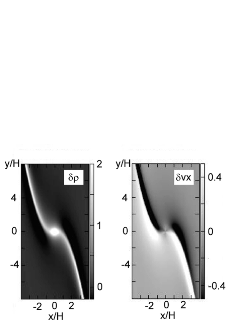
Figure 2.— Linear density perturbation $\delta\Sigma/\Sigma_{0}$ (left) and $\delta v_{x}$ (right). We use $GM_{\rm p}/Hc^{2}=1$, but the perturbation scales with the mass of the planet.

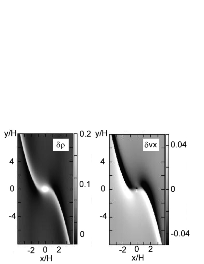
Figure 3.— Simulation results of $\delta\Sigma/\Sigma_{0}$ (left) and $\delta v_{x}$ (right) at $t\Omega_{\rm p}=200$. We use $GM_{\rm p}/Hc^{2}=0.1$.

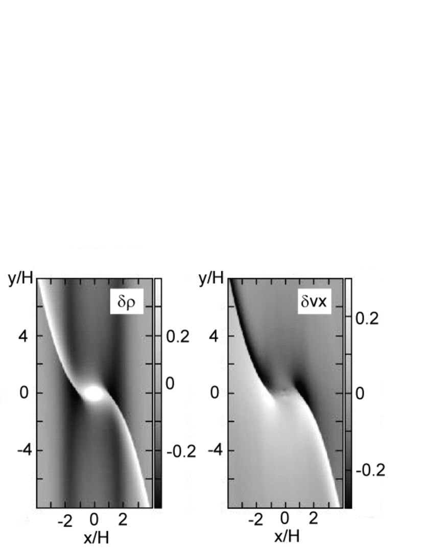
Figure 4.— Simulation results of $\delta\Sigma/\Sigma_{0}$ and $\delta v_{x}$ at $t\Omega_{\rm p}=200$. We use $GM_{\rm p}/Hc^{2}=0.4$.

Figure 5.— The evolution of azimuthally averaged density profile for $GM_{\rm p}/Hc^{2}=0.1$ (left) and $0.4$ (right).

Figure 6.— Density profile at $t\Omega_{\rm p}=200$. Profiles at $x/H=1$, $1.5$, $2$, $2.5$, and $3$ are shown from right to left. Left panel is for $GM_{\rm p}/Hc^{2}=0.1$ and the right panel is for $GM_{\rm p}/Hc^{2}=0.4$.

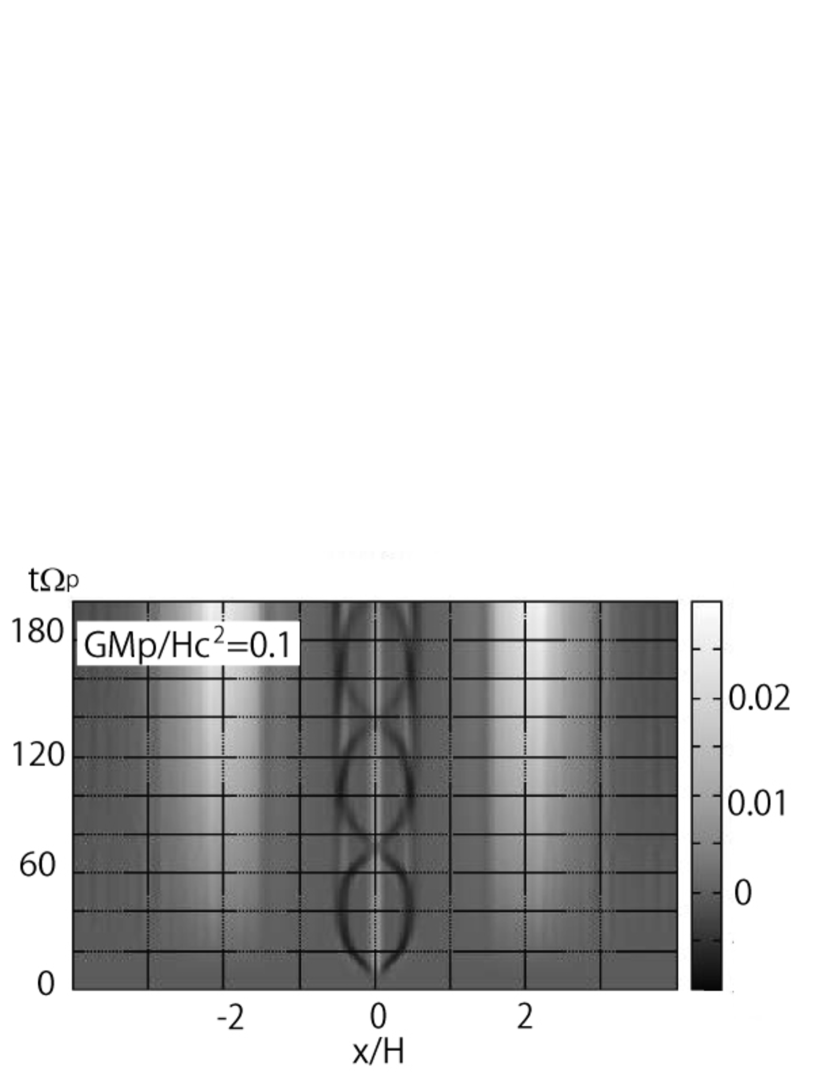
Figure 7.— Time evolution of azimuthally averaged specific vorticity perturbation for $GM_{\rm p}/Hc^{2}=0.1$ (left) and $0.4$ (right).

Figure 8.— Perturbation of specific vorticity (in arbitrary unit) as a function of $(x-(2H/3))\times M_{\rm p}^{2/5}$.

Figure 9.— Comparison between the mass flux obtained from numerical calculation (dots) and the fitting function (61) with $K=4.4\times 10^{-3}$. We plot the value $(GM_{\rm p}/Hc^{2})^{-2}(1/L_{y})\int dy\Sigma v_{x}$. Left panel shows the results with $GM_{\rm p}/Hc^{2}=0.1$ and the right panel shows the results with $GM_{\rm p}/Hc^{2}=0.4$. The horizontal axis shows $x/H$.

Figure 10.— Comparison of the mass flux obtained by numerical calculation and second-order perturbation theory. Left panel shows the result with $GM_{\rm p}/Hc^{2}=0.1$, and the right panel shows the results with $GM_{\rm p}/Hc^{2}=0.4$.

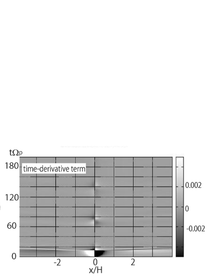
Figure 11.— The evolution of the source terms of mass flux obtained by the calculations with $GM_{\rm p}/Hc^{2}=0.1$. Left panel shows $S_{v}(t,x)$ given by equation (41). Right panel shows $\partial_{t}S_{t}(t,x)$ where $S_{t}(t,x)$ is given by equation (42).

Figure 12.— Mass flux obtained by second order perturbation theory. Solid line shows the case where the source term is restricted to $|x/H|<1$, while the dashed line shows the result with full source term.

Figure 13.— Integrated mass flux $\int dy\Sigma v_{x}$ for box sizes with $L_{y}/H=16,32,64,128$. The mass of the planet is $GM_{\rm p}/Hc^{2}=0.2$ and the data at $t\Omega_{\rm p}=100$ are used.

Figure 14.— Evolution of density profile (left) and the mass flux (right) for the calculation with $GM_{\rm p}/Hc^{2}=0.6$

Figure 15.— Comparison of each term in equation (A16). Data with $GM_{\rm p}/Hc^{2}=0.2$ at $t\Omega_{\rm p}=100$ is used. The line “(mass flux)/2” is the left hand side of equation (A16), “derivative of angular momentum flux” is the first term of the right hand side (sign inverted), and “torque” is the second term of the right hand side. The line “total” is the value when all the terms are taken to the left hand side, and should be zero if equation (A16) is strictly satisfied.

Table 1Mass parameters used in numerical calculations

Model Number	$GM{\rm p}/Hc^{2}$	Planet Mass	$r_{\rm H}/H$
1	0.05	$1.875M_{\oplus}$	0.26
2	0.1	$3.75M_{\oplus}$	0.32
3	0.2	$7.5M_{\oplus}$	0.41
4	0.4	$15M_{\oplus}$	0.51
5	0.6	$22.5M_{\oplus}$	0.58

References

- Abramowitz and Stegun (1970) Abramowitz, M. & Stegun, I. A. 1970, Handbook Of Mathematical Functions (New York: Dover)
- Artymowicz (1993) Artymowicz, P. 1993, ApJ, 419, 155
- Balbus and Papaloizou (1999) Balbus, S. A., & Papaloizou, J. C. B. 1999, ApJ, 521, 650
- Baruteau (2008) Baruteau, C. 2008, PhD. Thesis
- Chandrasekhar (1981) Chandrasekhar, S. 1981, Hydrodynamic and Hydromagnetic Stability, (New York: Dover)
- Colella and Woodward (1984) Colella, P., & Woodward, P. R. 1984, Journal Comp. Phys., 54, 174
- Crida et al. (2006) Crida, A., Morbidelli, A., & Masset, F. 2006, Icarus, 181, 587
- Goldreich and Tremaine (1979) Goldreich, P., & Tremaine, S. 1979, ApJ, 233, 857
- Goldreich and Tremaine (1980) Goldreich, P., & Tremaine, S. 1980, ApJ, 241, 425