Bayesian Tracking of Emerging Epidemics Using Ensemble Optimal Statistical Interpolation (EnOSI)

Abstract

We explore the use of the optimal statistical interpolation (OSI) data assimilation method for the statistical tracking of emerging epidemics and to study the spatial dynamics of a disease. The epidemic models that we used for this study are spatial variants of the common susceptible-infectious-removed (S-I-R) compartmental model of epidemiology. The spatial S-I-R epidemic model is illustrated by application to simulated spatial dynamic epidemic data from the historic ”Black Death” plague of 14th century Europe. Bayesian statistical tracking of emerging epidemic diseases using the OSI as it unfolds is illustrated for a simulated epidemic wave originating in Santa Fe, New Mexico.

1 Introduction

Mathematical models have been used since 1927 to describe the rise and fall of infectious disease epidemics (Diekmann and Heesterbeek, 2000; Castillo-Chávez and Blower, 2002a, b; Ma and Xia, 2009). A majority of the models are based on the three-compartment nonlinear Susceptible-Infected-Removed (S-I-R) model developed by Kermack and McKendrick (1927). A person occupies the susceptible or infectious compartments if he or she can contract or transmit the disease, respectively. The removed compartment includes those who have died, have been quarantined, or have recovered from the disease and become immune. The state variables are the number of susceptible ($S$), the infectious ($I$), and the removed ($R$) in a closed population. S-I-R models often perform surprisingly well in modeling the temporal evolution of real-world epidemics, and their spatial variants can produce a traveling-wave spatial dynamics similar to that displayed by some epidemics. Traveling waves are solutions to the spatial models such that the distribution of infected at time ($t+1$) is approximately a translation of the distribution at time $t$.

Tracking and forecasting the full spatio-temporal evolution of a new epidemic is notoriously difficult. Often the model itself is incorrect in unknown ways, observational data may be affected by many sources of error, and new data arrives on an irregular schedule. This is a well-known problem in a variety of empirical areas of high importance, such as storm and wildfire forecasting. The general category of tracking techniques that incorporate error-prone data as they arrive by sequential statistical estimation is known as data assimilation (Kalnay, 2003). Use of the statistical methods of data assimilation can increase the accuracy and reliability of epidemic tracking by incorporating data as it arrives, with weighting factors that reflect the observed reliability of the observations. A few applications of data assimilation in epidemiology already exist (Kalivianakis et al., 1994; Cazelles and Chau, 1997; Costa et al., 2005; Bettencourt et al., 2007; Bettencourt and Ribeiro, 2008; Jégat et al., 2008; Rhodes and Hollingsworth, 2009; Dukic et al., 2009; Mandel et al., 2010a).

The aim of this paper is to study the use of a spatial variant of the S-I-R model to track newly emerging epidemics using a data assimilation technique called optimal statistical interpolation (OSI). This is already a popular data assimilation method in the literature of meteorology and oceanography. When coupled with a spatial dynamic model, the OSI method can be used to forecast the spatio-temporal evolution of an epidemic, and to adjust those forecasts appropriately as sparse and error-prone data arrives.

This paper is organized as follows. In Section 2, we present a stochastic spatial epidemic model and use it to reproduce the spatio-temporal disease spread map of the 14th century Black Death. In Section 3, we illustrate the Bayesian tracking of emerging epidemics using OSI with a simulated epidemic wave originating in Santa Fe, New Mexico. In Section 4, we provide computational results for the stochastic spatial epidemic model with epidemic tracking method presented in Section 3. Finally, in Section 5, we provide some concluding remarks and future directions.

2 A Stochastic Spatial Epidemic Model

2.1 Epidemic Dynamics

For this study we use a discretized stochastic version of the Hoppensteadt (1975) spatial S-I-R epidemic model. As with almost all spatial epidemic models since Bailey (1957, 1967); Kendall (1965), we assume that individuals are continuously distributed on a spatial domain. This model uses three variables to define the state of the epidemic at each $(x,y)$ coordinate:

$\qquad S(x,y,t)=$ density (per unit area) of the susceptible population,

$\qquad I(x,y,t)=$ density of the infected population, and

$\qquad R(x,y,t)=$ density of the removed population.

Thus, each of these variables is a scalar field that evolves with time.

In continuous time the epidemic dynamics are defined by a system of three partial differential equations for the state variables. There are no vital dynamics in this model, meaning that there are no new births or non-disease related deaths in any of the three compartments. Following Hoppensteadt (1975), we assume that the rate of new infections at location $(x,y)$ depends on the density of infection at that point, and in nearby locations that have been weighted with a kernel function that drops off exponentially with Euclidean distance. The effective (i.e. weighted) density of infection at $(x,y)$ is given by

$$J(x,y,t) =\int\int I(x-\phi,y-\theta)K(\phi,\theta)d\phi d\theta,$$

$$K(\phi,\theta) \propto\exp\left(-\alpha\sqrt{\phi^{2}+\theta^{2}}\right),$$

where the integral is taken over the entire surface area under study, and the proportionality constant is given by the condition that $\int\int K(\phi,\theta)d\phi d\theta=1$. Then, the three partial differential equations for the deterministic evolution of the spatial epidemic are:

$$\partial_{t}S =-\beta SJ,$$

$$\partial_{t}I =\beta SJ-\gamma I,$$

$$\partial_{t}R =\gamma I.$$

In this model, $\beta$ is the rate of infection from infected to susceptibles, given homogeneous mixing, $\alpha$ is an intensity measure of infectiousness of the disease, given by the product of mixing rate and the infection rate and $\gamma$ is the rate of removal of infected persons through death, recovery with immunity, and quarantine. To make this model stochastic, we assume that the quantities $\beta SJ$ and $\gamma I$ are the intensities of two independent Poisson processes. For simulations in discrete time and space, we use the following approximation: The number of newly infected and newly removed persons over the time interval $(t,t+\Delta t)$, within a box centered at position $(x,y)$ with $\Delta x\Delta y$ units of area, are given by

Number newly infected $\sim Poisson(\beta S(x,y,t)J(x,y,t)\Delta x\Delta y\Delta t)$,

Number newly removed $\sim Poisson(\gamma I(x,y,t)\Delta x\Delta y\Delta t).$

Thus a susceptible individual, at a particular location, may become infected when he/she comes in contact with an infected individual from within a neighboring area, with a monotonically decreasing weighting function that declines exponentially with distance. If this contact causes sufficient secondary infections then a new epidemic focus will develop at that new location. The simulation evolves on a two-dimensional discretized spatial domain with a total of $n\times m$ grid cells.

2.2 Example: The Black Death in Europe

The ”Black Death” bubonic plague epidemic that hit Europe in 1347 killed somewhere between 30% and 60% of the population of Europe over the course of about four years. The virulence of the disease back then was severe, which explains the extremely high number of deaths. Plague recurred in various regions of Europe for another 300 years before gradually withdrawing from Europe. There have been several attempts to reconstruct the movement of the wavefront of the epidemic (Langer, 1964; Noble, 1974; Christakos and Olea, 2005; Christakos et al., 2007; Gaudart et al., 2010), as it swept across the continent; one such attempt using our spatial S-I-R model is shown in Figure 1b; others are similar. The disease arrived from Asia into Europe by trading ships, appearing first in Constantinople (modern Istanbul, Turkey) in 1347. From there it was carried by ship to Italy, France, Spain, and Croatia. Once ashore it moved inland (mainly in pneumonic form) at a speed that has been estimated at between 100 and 400 miles per year.

If it is to have credibility, a spatial epidemic model should be able to reproduce the principal historical features of the Black Death: its movement into the interior of Europe from the coastal cities, especially Marseilles, and movement up the island of Britain after its arrival in Bristol and London. Figure 1b shows the population density of infected people, using modern population densities in place of the unknown medieval population pattern, at roughly the beginning of 1350.

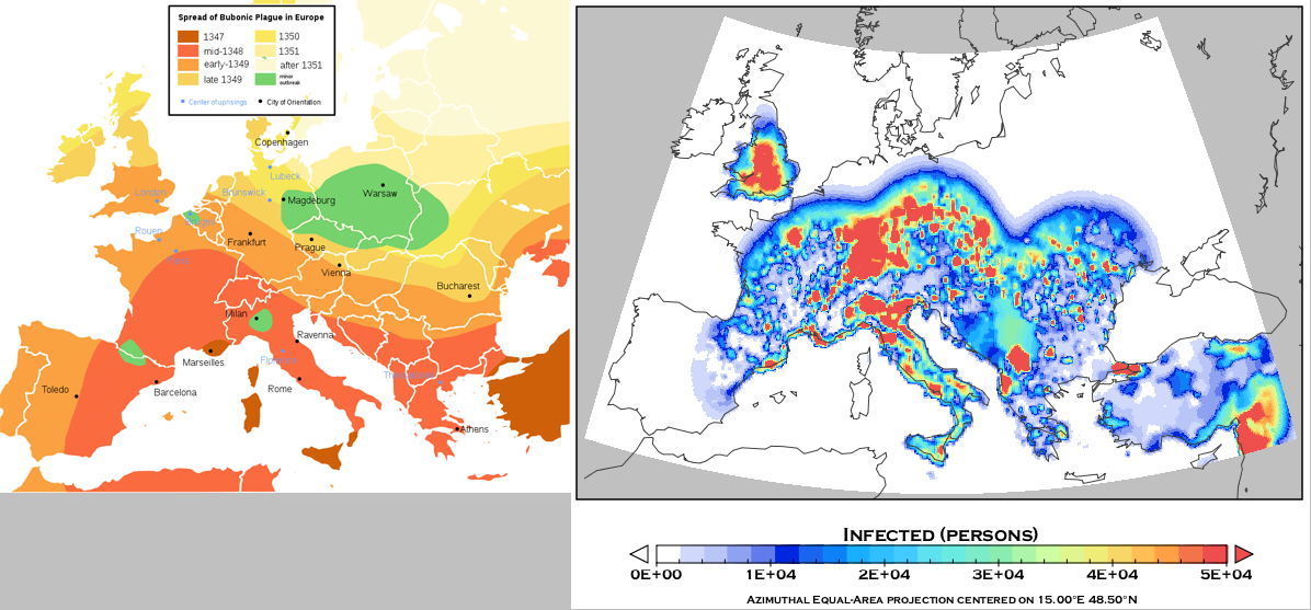
Figure 1: Figure 1a (left) Historical reconstruction. (Reproduced from Qedoc.org (2008) under Creative Commons license.) 1b (right) Simulated state of the epidemic in 1350.

The R statistical computing language (R Development Core Team, 2010), freely available from www.cran.r-project.org, was used to carry out the simulations for the spatial spread of the epidemic. Modern day population density data were downloaded as GPW (Gridded Population of the World) data files from the Center for International Earth Science Information Network at the Columbia University and converted to the array-oriented Network Common Data Form (NetCDF) format. These datasets were then loaded into R using the built-in package ncdf.

2.3 Comparison to Historical Data

In historical reality, the zone from Romania to Poland to Russia suffered only lightly from the first wave of the Black Death. It is quite plain that the S-I-R simulation does not conform to the historical reconstruction in that zone. The explanation may lie with the very low population density and geographic mobility in Eastern Europe in the 14th century. A smaller discrepancy occurs in the city of Milan, Italy, which brutally stopped the spread of the plague by boarding up infected people in their homes. Despite differences in population distribution (France was then much more populous than Germany, for example), we believe that the simulation performs reasonably well in all areas except Eastern Europe.

3 Statistical Tracking Using Data Assimilation Techniques

We use data assimilation for the statistical tracking of emerging epidemics as they are unfolding. This involves two basic components: a dynamic model to forecast the state of the epidemic between arrivals of new data, and observations that are used to update an ensemble of state estimates. Data assimilation requires estimating the uncertainty both for model and observations forecasts. Our goal in this paper is to incorporate sparse and noisy observational epidemic data over space and time into a dynamic statistical model so as to produce an optimal Bayesian estimate of the current state of the infected population, and to forecast the progress of the real epidemic.

3.1 The Kalman Filter (KF)

The Kalman Filter (KF) was first presented by Kalman (1960) and Kalman and Bucy (1961) as a method for tracking the state of a linear dynamic system perturbed by Gaussian white noise. In mathematical terms, this means that the errors are drawn from a zero-mean distribution with diagonal covariance matrix.

The full state of a discretized spatial epidemic model is a grid of $n\times m$ cells, each of which contains a characterization of the population currently within the limits of the cell. To apply the Kalman filtering method, we represent the $n\times m$ values of the Infected variable on this grid as a single long vector $x$ with $p=n\times m$ elements, which for the purposes of data assimilation is the dimensionality of the state space. If we could observe this state vector without error, our observations would be another vector $y$ that satisfies $y=Hx$. Now consider the situation in which we have a forecast of the current state, $x^{f}$, and a newly arrived vector of noisy observations $y=Hx+\varepsilon$, where $\varepsilon\sim N\left(0,R\right)$. We need to update the forecast by optimally assimilating these new observations. The result will be called the analysis estimate of state, $x^{a}$. The superscripts $f$ and $a$ are used to denote the forecast (prior) and analysis (posterior) estimate of the current state, respectively.

In the classical Kalman filter, the underlying dynamics are assumed to be linear, e.g.

$$x_{t} =F_{t-1}x_{t-1}+u_{t-1},$$

$$u_{t} \sim N\left(0,\Sigma\right),$$

and the analysis estimate of the state vector is calculated from

$$x_{t}^{f} =F_{t-1}x_{t-1}^{f}$$

$$x_{t}^{a} =x_{t}^{f}+K_{t}(y_{t}-Hx_{t}^{f}),$$

$$Q_{t}^{a} =(I-K_{t}H)Q_{t}^{f},$$

where

$$K_{t} =Q_{t}^{f}H^{T}(HQ_{t}^{f}H^{T}+R)^{-1},\text{ and}$$

$$Q_{t}^{f} =F_{t-1}Q_{t-1}^{f}F_{t-1}^{\prime}+\Sigma.$$

Here $K_{t}$ is the Kalman gain matrix at time $t$, and $Q_{t}^{f}$ is the covariance matrix for the forecast state vector.

The extended Kalman filter (EKF) (Julier et al., 1995) was an early attempt to adapt the basic KF equations for nonlinear problems, through linearization. However, the EKF has it’s own disadvantages: if the model is strongly nonlinear at the time step of interest, linearization errors can turn out to be non-negligible, which leads to filter divergence (Evensen, 1992). The EKF is not suitable for high-dimensional 2D and 3D data assimilation problems. Other commonly used Bayesian tracking techniques for nonlinear problems include the unscented Kalman filter (UKF) and the particle filter (PF) (Gordon et al., 1993). Particle filtering is a versatile Monte Carlo technique that can handle nonlinearities in the model and represents the Bayesian posterior probability density function by a set of samples drawn at random with associated weights.

3.2 Ensemble Kalman Filter (EnKF)

The KF algorithm described above is based on assimilating only one initial state ignoring the uncertainties in the model. In the following, we account for this state-dependent uncertainty by taking an ensemble approach to data assimilation. To see the problem, consider a 2D simulation of a scalar field that has been discretized on a $10^{3}\times 10^{3}$ grid. The state vector of this system has $10^{6}$ elements, and its covariance matrix has $10^{6}\times 10^{6}=10^{12}$ elements, requiring eight terabytes just to store. The EnKF solves this storage-and-retrieval problem by (in effect) calculating the covariances from the members of the ensemble as they are needed. The result is in an elegant Bayesian update algorithm with dramatically improved efficiency and storage requirements Mandel et al. (2010a).

The ensemble Kalman filter (EnKF) was introduced by Evensen (1994), modified to provide correct covariance by Burgers et al. (1998), and improved by Houtekamer and Mitchell (1998). The EnKF is a popular sequential Bayesian data assimilation technique that uses a collection of almost-independent simulations (known as an ensemble) to solve the covariance problem of Kalman filtering for systems with very high-dimensional state vectors. It does this using a two-step process: estimate of the covariance matrix, followed by an ensemble update. The covariance of a single state estimate in the KF is replaced by the sample covariance computed from the ensemble members. This sample covariance of ensemble forecasts is then used to calculate the Kalman gain matrix. There are two basic approaches to the EnKF update: stochastically perturbed observations (Monte Carlo), and “square-root” filters (deterministic). Both approaches adopt the same covariance estimate step, but differ in the ensemble update step. Regardless of the specific approach employed, the goal is to obtain a Bayesian estimate of the state as efficiently as possible. In many real-world examples these two approaches perform quite similarly. A more detailed description EnKF may be found in the book by Evensen (2009).

The EnKF analysis update equations are analogous to the classical KF equations, except that they use the covariance of the forecast ensemble to substitute for the matrix $Q$, which in a high-dimensional system is too large to store. Let $X$ be a random ensemble matrix of dimension $p\times N$ whose columns are realizations sampled from the prior distribution of the system state of dimension $p$ with ensemble size $N$. Then the EnKF update formula is:

$$X^{a}=X^{f}+K_{e}(Y-HX^{f}),$$

where $Y$ is the observed ensemble data matrix whose columns are the true state perturbed by random Gaussian error. $H$ is, as before, the linear operator that maps the state vector onto the observational space. The deviation $Y-HX^{f}$ is commonly referred to as the “observed-minus-forecast residual” or simply as the innovation. In the above equation $K_{e}$ is the ensemble Kalman gain matrix given by

$$K_{e}=Q^{f}H^{T}(HQ^{f}H^{T}+R)^{-1},$$

where $Q^{f}$ is the forecast-error covariance matrix of dimension $p\times p$, and $R$ is the symmetric and positive-definite observational (measurement) error covariance matrix. The EnKF technique contains two sources of randomness: the random model input, and the measurement errors. Assuming that these two sources of randomness are uncorrelated, the analysis-error covariance matrix of dimension $p\times N$ can be computed from the equation

$$Q^{a}=(I-K_{e}H)Q^{f}.$$

3.3 Optimal Statistical Interpolation (OSI)

In the EnKF, the model error covariance matrix is evolved fully at each data assimilation step using an MCMC method. In contrast, Optimal Statistical Interpolation (OSI) is a data assimilation technique based on statistical estimation theory in which the model error covariance matrix is pre-determined empirically and is assumed to be time-invariant. The model error covariance matrix is dependent only on the distance between spatial grid cells. The correlation length is ad hoc and adjusted empirically.

OSI was derived by Eliassen (1954). This method has been referred to as “Statistical Interpolation”, “Optimal Interpolation”, or “Objective Analysis.” OSI is called univariate if the observations are of a single scalar field, and multivariate if the observations of one or more scalar fields are used for estimating another scalar field (Talagrand, 2003). Multivariate OSI was developed independently by Gandin (1965) for the analysis of meteorological fields in the former Soviet Union. It requires the specification of the cross-covariance matrix between the observed scalar fields and the scalar field to be estimated.

The ensemble OSI (EnOSI), used here, requires much less computational effort than the EnKF, because the model error covariance matrix is fixed. The EnOSI approach may provide a practical and cost-effective alternative to the EnKF for tracking epidemics. The stationary model error covariance matrix in our epidemic simulation used a version with the correlation function having an exponential decay along the off-diagonal entries. The ensemble Kalman gain matrix was then calculated using this time-invariant covariance matrix with a fixed structure. The accuracy of the EnOSI process will be affected if the approximate covariance matrix differs substantially from the true covariance matrix. Therefore, one disadvantage of the OSI is the need for a fixed spatial covariance structure that can reasonably represent the epidemic dynamics throughout the whole domain at all times.

The EnOSI analysis update equation, using the stationary covariance, is given by

$$X^{a}=X^{f}+K_{OSI}(Y-HX^{f})$$ (1)

where

$$K_{OSI}=Q_{OSI}^{f}H^{T}(HQ_{OSI}^{f}H^{T}+R)^{-1}.$$

3.4 Example: An Epidemic Wave Originating In New Mexico

To test the performance of EnOSI and other tracking algorithms designed for high-dimensional state vectors, we constructed a spatial simulation of an epidemic that originates in Santa Fe, New Mexico, and spreads outwards towards Albuquerque and Denver, Colorado. In this simulation the epidemic moves smoothly towards Albuquerque, but jumps suddenly to to Denver as if carried by a traveler in an automobile or airplane. Properly detecting and assimilating a new feature far from an existing focus is a serious challenge for EnKF algorithms (Beezley and Mandel, 2008; Mandel et al., 2010a).

To improve the realism of the test for the case in which an entirely new disease emerges for the first time, we initialized all members of the tracking ensemble so that they contain no disease whatsoever. New data in the form of an empirical scalar field arrives at time steps 10, 20, 30, 40, and 50. These data are complete in the sense that in this case $H$ is just the identity matrix, but they are substantially modified by independent Poisson-distributed random errors. The tracking algorithm forecasts the state up until the time when data is received, and then it assimilates this data into the forecast.

4 Results

We have applied the EnOSI for the New Mexico example mentioned above to the epidemic model described in Section 2 with an ensemble of size 25. For this example the Infected state of the model is the output of the observation function. Synthetic data were simulated from a model and initialized in exactly the same way as the ensemble.

In our epidemics application, the perturbed observations $Y$ in (1) were obtained by sampling from the Poisson distribution with the intensity equal to the data value and rounding to integer, consistently with the stochastic character of the model, instead of Gaussian perturbations as in the EnKF. This is the key feature behind the successful use of our method and it also guarantees that $Y$ has nonnegative entries and thus the columns of $Y$ are meaningful as the Infected variable. In general, one may have to guarantee that the entries of the members of the analysis ensemble $X^{a}$ are also nonnegative, e.g. by censoring. This, however, was not needed in the results reported here.

The result for each member of the ensemble advanced in time by 10 model time units is a Bayesian update of the forecast scalar field, which is referred to as the analysis (i.e. the posterior estimate). We assume that data arrive only once every 10 time steps, with errors. A total of 5 assimilation cycles were performed in this manner. The mean and standard deviation (not reported here) of the ensemble analysis values in each cell of the scalar field gives the EnOSI estimate of the state of the epidemic, with its uncertainty quantified. The following figures present a spatial “image” of the number of infected persons over the planar domain considered in the New Mexico example.

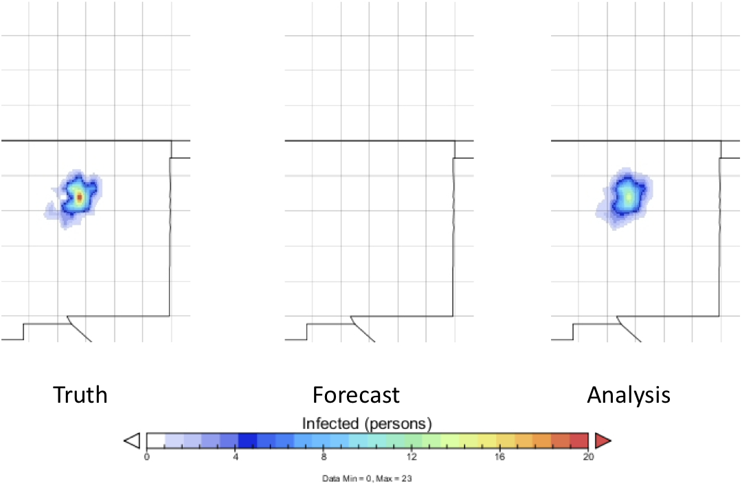
Figure 2: The epidemic at time 10. (a): The true state of the epidemic.(b): The forecast state of the epidemic prior to arrival of the first data. (c): The analysis state of the epidemic, after data assimilation.

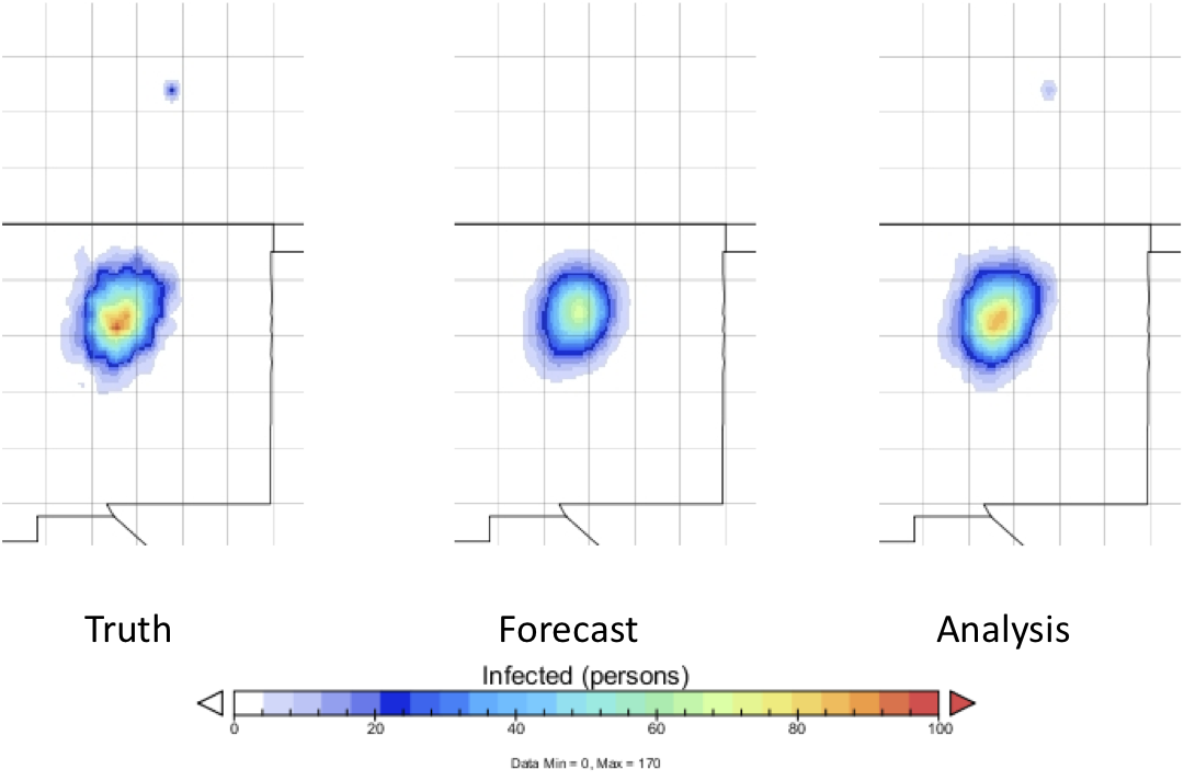
Figure 3: The epidemic at time 20. A new focus of infection has appeared in Denver, and is successfully reflected in the analysis state.

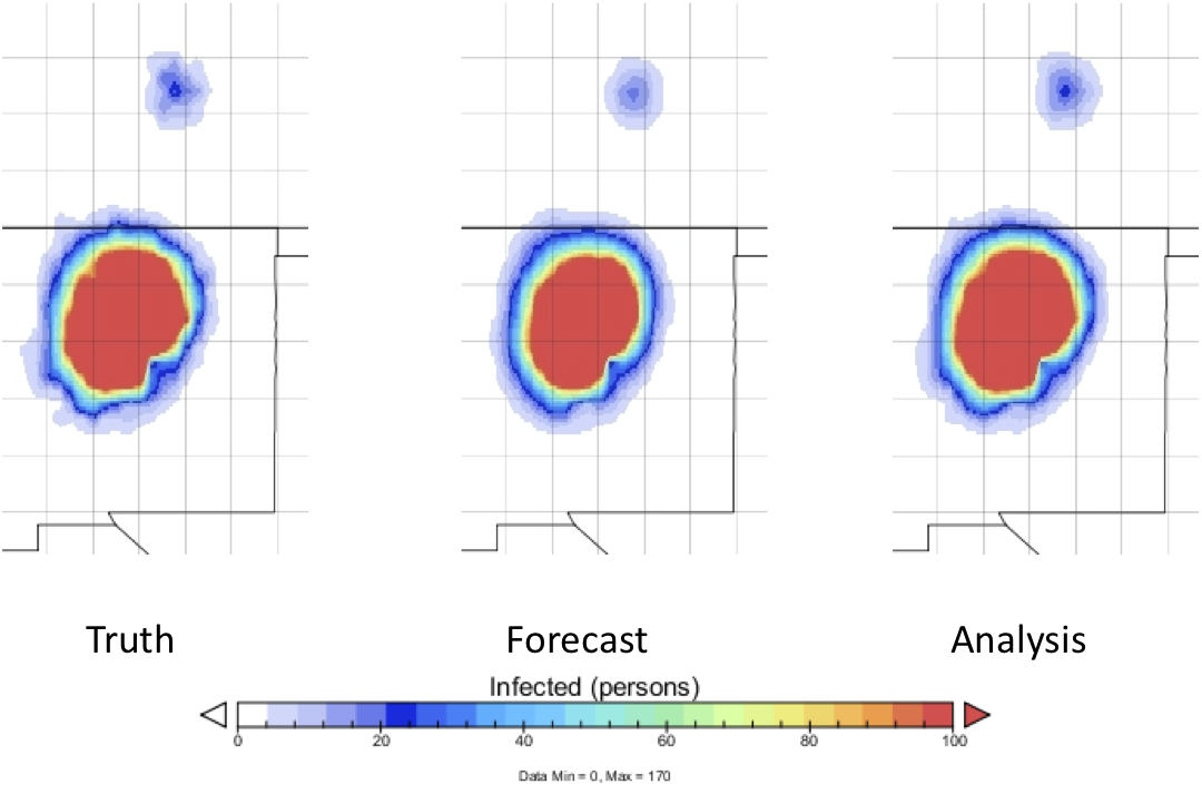
Figure 4: The epidemic at time 30. The infected zone is expanding rapidly.

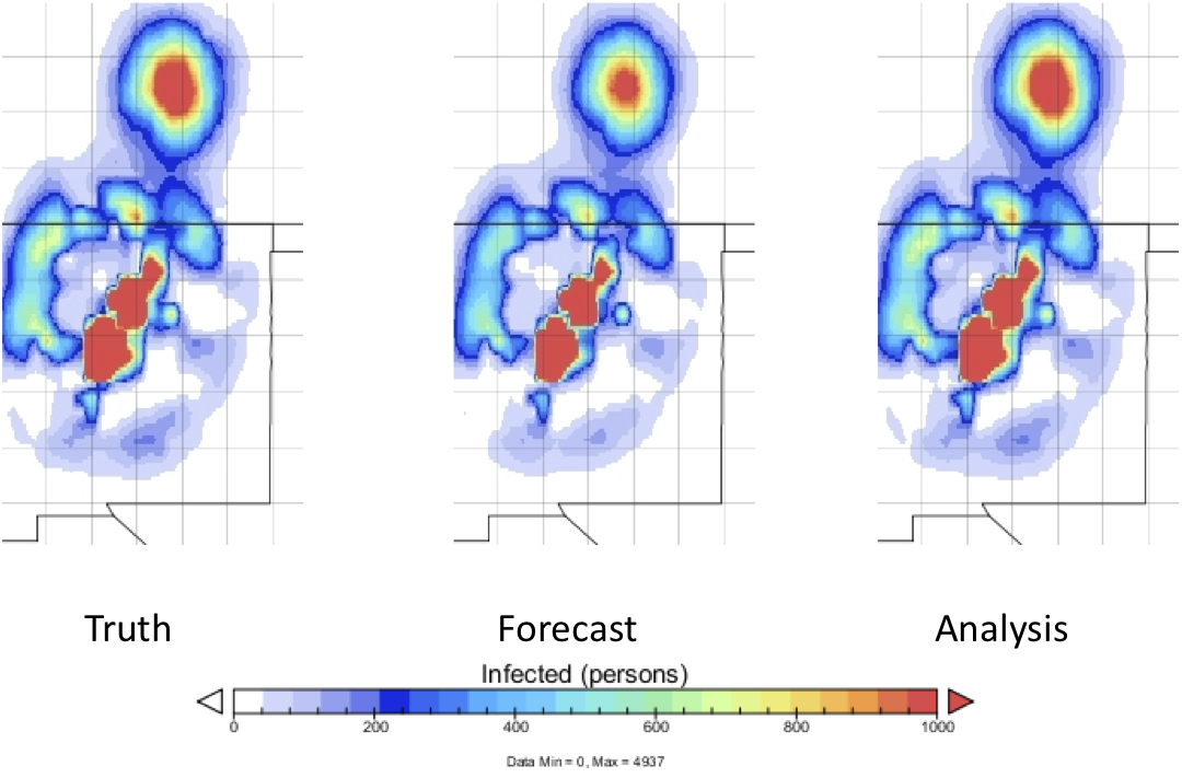
Figure 5: The epidemic at time 50. Both the forecast and analysis estimates of state now accurately reflect the true state of the epidemic.

Figure 2a shows the epidemic position in Santa Fe, New Mexico, at time 10. The initial forecast (2b) is empty, as it should be for the first appearance of any newly emergent disease. The EnOSI analysis (2c) shows that the arriving data have been partially assimilated, with a resulting picture that is indistinct and less than fully accurate. Figure 3a (time 20) shows the growth of the epidemic towards Albuquerque, and a very small new focus of infection in Denver. The forecast handles the movement towards Albuquerque quite well, but is devoid of any infection in Denver. After assimilation of the data, the analysis now also reflects a small focus in Denver. Figure 4 (time 30) shows the epidemic gaining size, and beginning a major expansion within both Albuquerque and Denver. Figure 5 (time 50) shows the epidemic gaining definition within the most heavily populated urban regions. The analysis steps, after data assimilation, are now tracking the epidemic quite well.

5 Conclusion

The spread of newly emerging infectious diseases pose a serious challenge to public health in every country of the world. Tracking the spread of an epidemic in real-time can help public health officials to plan their emergency response and health care. The purpose of this paper has been to present the some preliminary results on the statistical tracking of emerging epidemics of infectious diseases using a Bayesian data assimilation technique called ensemble optimal statistical interpolation (EnOSI). Our simulation results confirms that EnOSI can be used to track the spatio-temporal patterns of emerging epidemics. We found that EnOSI can efficiently adjust its estimated spatial distribution of the number of infected, if and when the epidemic jumps from city to city, and with data that are sparse and error-ridden. The tracking accuracy in our simulations provides evidence of the good performance of the EnOSI approach, therefore the assumption that the model error covariance is time-invariant is reasonable. However, the effect of this assumption needs more rigorous theoretical justification.

The EnOSI as presented here requires the manipulation of the state covariance matrix, which gets very demanding if stored as a full matrix - computational grid of 200 by 200 points results in 40,000 variables and thus 40,000 by 40,000 covariance matrix, which requires a supercomputing cluster. Sparsification of the covariance matrix can decrease the computational cost somewhat, but it is still significant and the implementation grows complicated. For this reason, we plan to investigate a version of OSI by Mandel (2010) with the covariance implemented by the Fast Fourier Transform (FFT), similarly as in the FFT EnKF Mandel et al. (2010a, b, c).

Our research has set the groundwork for further efforts to incorporate the ideas of data assimilation to track diseases in real-time. Our future work includes extending the R framework that we have developed for employing an ensemble of spatial simulations to track diseases to test and compare a other variants of the EnKF (Anderson, 2001; Tippett et al., 2003; Beezley and Mandel, 2008; Mandel et al., 2009a; Ott et al., 2004; Hunt et al., 2007). These variants aim to enhance the performance of the ensemble filters by representing the underlying model error statistics in an efficient manner. However, since the ensemble size required can be large (easily hundreds) Evensen (2009) for the approximation to converge (Mandel et al., 2009b), the amount of computations in the ensemble-based methods can be significant, and so special localization techniques, such as tapering, need to be employed to suppress spurious long-range correlations in the ensemble covariance matrix (Furrer and Bengtsson, 2007). Thus the EnKF (and its variants) may not work well for problems with sharp coherent features, such as the traveling waves found in some epidemics. Choosing a small ensemble size, so small that it is not statistically representative of the state of a system, leads to underestimation of the analysis error covariances. Choosing a really large ensemble size may not be computationally feasible and cost efficient. Finally, methods for incorporating long-distance human movements to track the rapid geographical spread of infectious diseases have been proposed in the literature (Brockmann, 2009; Belik et al., 2009; Merler and Ajelli, 2010; Balcan et al., 2010; Belik et al., 2010). In the future, we plan to explore such spatially extended epidemic models to track emerging epidemics.

References

- Anderson (2001) Anderson, J. L. (2001), “An ensemble adjustment Kalman filter for data assimilation,” Monthly Weather Review, 129, 2884–2903.
- Bailey (1957) Bailey, N. T. J. (1957), Mathematical Theory of Epidemics, Griffin.
- Bailey (1967) — (1967), “The simulation of stochastic epidemics in two dimensions,” in Proceedings of the fifth Berkeley Symposium on mathematical statistics and probability: biology and problems of health, vol. 4, pp. 237–257.
- Balcan et al. (2010) Balcan, D., Gonçalves, B., Hu, H., Ramasco, J. J., Colizza, V., and Vespignani, A. (2010), “Modeling the spatial spread of infectious diseases: The Global Epidemic and Mobility computational model,” Journal of Computational Science.
- Beezley and Mandel (2008) Beezley, J. D. and Mandel, J. (2008), “Morphing ensemble Kalman filters,” Tellus A, 60, 131–140.
- Belik et al. (2009) Belik, V., Geisel, T., and Brockmann, D. (2009), “The impact of human mobility on spatial disease dynamics,” in Proceedings of the 2009 International Conference on Computational Science and Engineering-Volume 04, IEEE Computer Society, pp. 932–935.
- Belik et al. (2010) — (2010), “Human movements and the spread of infectious diseases,” NetMob 2010: Workshop on the Analysis of Mobile Phone Networks, 44–48.
- Bettencourt and Ribeiro (2008) Bettencourt, L. M. A. and Ribeiro, R. M. (2008), “Real time bayesian estimation of the epidemic potential of emerging infectious diseases,” PLoS One, 3, 1–9.
- Bettencourt et al. (2007) Bettencourt, L. M. A., Ribeiro, R. M., Chowell, G., Lant, T., and Castillo-Chavez, C. (2007), “Towards real time epidemiology: data assimilation, modeling and anomaly detection of health surveillance data streams,” in Intelligence and Security Informatics: Biosurveillance, Springer, vol. 4506 of Lecture Notes in Computer Science, pp. 79–90.
- Brockmann (2009) Brockmann, D. (2009), Human mobility and spatial disease dynamics, Wiley-VCH, pp. 1–24.
- Burgers et al. (1998) Burgers, G., van Leeuwen, P. J., and Evensen, G. (1998), “Analysis scheme in the ensemble Kalman filter,” Monthly Weather Review, 126, 1719–1724.
- Castillo-Chávez and Blower (2002a) Castillo-Chávez, C. and Blower, S. (2002a), Mathematical Approaches for Emerging and Reemerging Infectious Diseases: An Introduction, Springer Verlag.
- Castillo-Chávez and Blower (2002b) — (2002b), Mathematical Approaches for Emerging and Reemerging Infectious Diseases: Models, Methods and Theory, Springer Verlag.
- Cazelles and Chau (1997) Cazelles, B. and Chau, N. P. (1997), “Using the Kalman filter and dynamic models to assess the changing HIV/AIDS epidemic,” Mathematical Biosciences, 140, 131–154.
- Christakos and Olea (2005) Christakos, G. and Olea, R. A. (2005), “New space-time perspectives on the propagation characteristics of the Black Death epidemic and its relation to bubonic plague,” Stochastic Environmental Research and Risk Assessment, 19, 307–314.
- Christakos et al. (2007) Christakos, G., Olea, R. A., and Yu, H. L. (2007), “Recent results on the spatiotemporal modelling and comparative analysis of Black Death and bubonic plague epidemics,” Public Health, 121, 700–720.
- Costa et al. (2005) Costa, P. J., Dunyak, J. P., and Mohtashemi, M. (2005), “Models, prediction, and estimation of outbreaks of infectious disease,” IEEE SoutheastCon, 2005. Proceedings, 174–178.
- Diekmann and Heesterbeek (2000) Diekmann, O. and Heesterbeek, J. (2000), Mathematical epidemiology of infectious diseases. Model building, analysis and interpretation, Wiley Series in Mathematical and Computational Biology.
- Dukic et al. (2009) Dukic, V. M., Lopes, H. F., and Polson, N. (2009), “Tracking Flu Epidemics Using Google Flu Trends and Particle Learning,” SSRN eLibrary, http://ssrn.com/paper=1513705.
- Eliassen (1954) Eliassen, A. (1954), “Provisional Report on Calculation of Spatial Covariance and Autocorrelation of the Pressure Field.” Rept. No. 5, Institute of Weather and Climate Research, Academy of Sciences, Oslo, reprinted in Dynamic Meteorology: Data Assimilation Methods, L. Bengtsson, M. Ghil, and E. Kallen., Ed., Springer-Verlag, 319–330, 1981.
- Evensen (1992) Evensen, G. (1992), “Using the Extended Kalman Filter With a Multilayer Quasi-Geostrophic Ocean Model,” J. Geophys. Res, 97, 17905–17924.
- Evensen (1994) — (1994), “Sequential data assimilation with a nonlinear quasi-geostrophic model using Monte Carlo methods to forecast error statistics,” J. Geophys. Res, 99, 10143–10162.
- Evensen (2009) — (2009), Data assimilation: The ensemble Kalman filter, Springer Verlag.
- Furrer and Bengtsson (2007) Furrer, R. and Bengtsson, T. (2007), “Estimation of high-dimensional prior and posterior covariance matrices in Kalman filter variants,” Journal of Multivariate Analysis, 98, 227 – 255.
- Gandin (1965) Gandin, L. S. (1965), Objective analysis of meteorological fields, English translation from the Russian by Israel Program for Scientific Translations.
- Gaudart et al. (2010) Gaudart, J., Ghassani, M., Mintsa, J., Waku, J., Rachdi, M., Doumbo, O. K., and Demongeot, J. (2010), “Demographic and Spatial Factors as Causes of an Epidemic Spread, the Copule Approach: Application to the Retro-prediction of the Black Death Epidemy of 1346,” in 2010 IEEE 24th International Conference on Advanced Information Networking and Applications Workshops, IEEE, pp. 751–758.
- Gordon et al. (1993) Gordon, N. J., Salmond, D. J., and Smith, A. F. M. (1993), “Novel approach to nonlinear/non-Gaussian Bayesian state estimation,” in IEE Proceedings, vol. 140, pp. 107–113.
- Hoppensteadt (1975) Hoppensteadt, F. (1975), Mathematical Theories of Populations, Demographics, and Epidemics, CBMS-NSF Regional Conference Series in Applied Mathematics, SIAM.
- Houtekamer and Mitchell (1998) Houtekamer, P. L. and Mitchell, H. L. (1998), “Data Assimilation Using an Ensemble Kalman Filter Technique,” Monthly Weather Review, 126, 796–811.
- Hunt et al. (2007) Hunt, B. R., Kostelich, E. J., and Szunyogh, I. (2007), “Efficient data assimilation for spatiotemporal chaos: A local ensemble transform Kalman filter,” Physica D: Nonlinear Phenomena, 230, 112–126.
- Jégat et al. (2008) Jégat, C., Carrat, F., Lajaunie, C., and Wackernagel, H. (2008), “Early Detection and Assessment of Epidemics by Particle Filtering,” in GeoENV VI-Geostatistics for Environmental Applications: Proceedings of the Sixth European Conference on Geostatistics for Environmental Applications, Springer Verlag, pp. 23–35.
- Julier et al. (1995) Julier, S. J., Uhlmann, J. K., and Durrant-Whyte, H. F. (1995), “A new approach for filtering nonlinear systems,” in Proc. American Control Conf, vol. 3, pp. 1628–1632.
- Kalivianakis et al. (1994) Kalivianakis, M., Mous, S. L. J., and Grasman, J. (1994), “Reconstruction of the seasonally varying contact rate for measles,” Mathematical biosciences, 124, 225–234.
- Kalman and Bucy (1961) Kalman, R. and Bucy, R. (1961), “New results in linear prediction and filtering theory,” Trans. AMSE J. Basic Eng, 95–108.
- Kalman (1960) Kalman, R. E. (1960), “A new approach to linear filtering and prediction problems,” Journal of basic Engineering, 82, 35–45.
- Kalnay (2003) Kalnay, E. (2003), Atmospheric modeling, data assimilation, and predictability, Cambridge Univ Pr.
- Kendall (1965) Kendall, D. G. (1965), “Mathematical models of the spread of infection,” Mathematics and Computer Science in Biology and Medicine, 213.
- Kermack and McKendrick (1927) Kermack, W. O. and McKendrick, A. G. (1927), “A Contribution to the Mathematical Theory of Epidemics,” Royal Society of London Proceedings Series A, 115, 700–721.
- Langer (1964) Langer, W. L. (1964), “The Black Death,” Scientific American, 210, 114.
- Ma and Xia (2009) Ma, S. and Xia, Y. (2009), Mathematical Understanding of Infectious Disease Dynamics, World Scientific.
- Mandel (2010) Mandel, J. (2010), “Osimorph,” http://ccm.ucdenver.edu/wiki/Osimorph.
- Mandel et al. (2010a) Mandel, J., Beezley, J. D., Cobb, L., and Krishnamurthy, A. (2010a), “Data driven computing by the morphing fast Fourier transform ensemble Kalman filter in epidemic spread simulations,” Procedia Computer Science, 1, 1215 – 1223, ICCS 2010.
- Mandel et al. (2009a) Mandel, J., Beezley, J. D., Coen, J. L., and Kim, M. (2009a), “Data Assimilation for Wildland Fires: Ensemble Kalman filters in coupled atmosphere-surface models,” IEEE control systems, 29, 47–65.
- Mandel et al. (2010b) Mandel, J., Beezley, J. D., Eben, K., Jurus, P., Kondratenko, V. Y., and Resler, J. (2010b), “Data assimilation by morphing fast Fourier transform ensemble Kalman filter for precipitation forecasts using radar images,” CCM UCD Report 290, http://ccm.ucdenver.edu/reports.
- Mandel et al. (2010c) Mandel, J., Beezley, J. D., and Kondratenko, V. Y. (2010c), “Fast Fourier Transform Ensemble Kalman Filter with Application to a Coupled Atmosphere-Wildland Fire Model,” in Computational Intelligence in Business and Economics, Proceedings of MS10, ed. A. M. Gil-Lafuente, J. M. M., World Scientific, pp. 777–784, also available as preprint arXiv:1001.1588.
- Mandel et al. (2009b) Mandel, J., Cobb, L., and Beezley, J. (2009b), “On the convergence of the ensemble Kalman filter,” Applications of Mathematics, in print, also available as arXiv:0901.2951.
- Merler and Ajelli (2010) Merler, S. and Ajelli, M. (2010), “The role of population heterogeneity and human mobility in the spread of pandemic influenza,” Proceedings of the Royal Society B: Biological Sciences, 277, 557–565.
- Noble (1974) Noble, J. V. (1974), “Geographic and temporal development of plagues,” Nature, 250, 726–729.
- Ott et al. (2004) Ott, E., Hunt, B., Szunyogh, I., Zimin, A., Kostelich, E., Corazza, M., Kalnay, E., Patil, D., and Yorke, J. (2004), “A local ensemble Kalman filter for atmospheric data assimilation,” Tellus A, 56, 415–428.
- Qedoc.org (2008) Qedoc.org (2008), “Diffusion de la peste noire en europe 1347-1351,” http://www.qedoc.org/en/index.php?title=Educational_Media_Awareness_Cam%paign/History/POTD_5, visited September 2010.
- R Development Core Team (2010) R Development Core Team (2010), R: A Language and Environment for Statistical Computing, R Foundation for Statistical Computing, Vienna, Austria.
- Rhodes and Hollingsworth (2009) Rhodes, C. J. and Hollingsworth, T. D. (2009), “Variational data assimilation with epidemic models,” Journal of Theoretical Biology, 258, 591–602.
- Talagrand (2003) Talagrand, O. (2003), “Bayesian estimation. Optimal interpolation. Statistical linear estimation,” in Data assimilation for the Earth system, eds. Swinbank, R., Shutaev, V. P., and Lahoz, W. A., Springer Netherlands, pp. 21–35.
- Tippett et al. (2003) Tippett, M. K., Anderson, J. L., Bishop, C. H., Hamill, T. M., and Whitaker, J. S. (2003), “Ensemble Square Root Filters,” Monthly Weather Review, 131, 1485–1490.