Bang-Bang Control Design for Quantum State Transfer based on Hyperspherical Coordinates and Optimal Time-energy Control

Abstract

We present a constructive control scheme for solving quantum state engineering problems based on a parametrization of the state vector in terms of complex hyperspherical coordinates. Unlike many control schemes based on factorization of unitary operators, the scheme gives explicit expressions for all generalized Euler angles in terms of the hyperspherical coordinates of the initial and final states. The factorization, when applicable, has added benefits that phase rotations can be combined and performed concurrently. The control procedure can be realized using simple bang-bang or square-wave-function controls. Optimal time-energy control is considered to find the optimal control amplitude. The extension of the scheme to implement arbitrary unitary operators is also discussed.

Keywords: quantum systems, Bang-Bang control, geometric parametrization, controllability, optimal control

1 Introduction

Control of phenomena governed by the laws of quantum mechanics is increasingly recognized as a crucial task and prerequiste to realizing promising new technologies based on quantum effects from the use of photonic reagents in chemistry [1] to quantum metrology and quantum information processing [2] to mention only a few examples. From early beginnings in the 1980s (see e.g., [3, 4, 5, 6, 7]), there has been considerable recent progress in both theory and experiment of quantum control [8, 9]. Among the core tasks for quantum control are quantum state and operator engineering. In the former case the main objective is to prepare the system in a desired state, which is usually a pure state $|\psi_{f}\rangle$ represented by a unit vector in a Hilbert space $\mathcal{H}$ associated with the system. The task can take various forms, from state transfer, i.e., steering the system from a known initial state $|\psi_{0}\rangle$ to the target state [10, 11, 12, 13, 14], to purification or state reduction, i.e., preparation of a desired pure state starting with a mixed or unknown initial state, usually involving some form of feedback from measurements of an observable [15, 16, 17], to protecting or stabilizing a desired state in the presence of environment noise or disturbance [18, 19, 20]. Often the goal is the preparation of a non-classical state such as a Greenberger-Horne-Zeilinger (GHZ) state [21], or a maximally entangled Bell state [22]. Operator engineering usually involves engineering the dynamical evolution to realize a particular unitary operator [23, 24, 25, 26, 27], and plays a crucial role in the implementation of quantum gates in the context for quantum information processing.

Some of the tasks mentioned above such as purification or stabilization generally require measurements and feedback [15, 16, 17], or possibly coherent feedback [31, 32], and some proposed control strategies actively take advantage of environmental effects [28, 29, 30] or even backaction effects of measurements and feedback [18, 19]. Perhaps the majority of control strategies for quantum dynamics, at least to date, however, rely on coherent open-loop control, i.e., manipulation of the dynamics via coherent interaction of the system with external fields or potentials, the type of control that we will be considered in this article. The main reason for foregoing measurements and feedback is to avoid the disturbance of the system that results from the backaction of measurement and feedback on the system, leading to complex non-unitary dynamics and decoherence. The challenge of open-loop control is to design external fields or potentials acting as controls off-line based on a model of the system. The main strategies for control design in this context are based either on geometric ideas, or more formally Lie group decompositions, as in [23, 24, 25, 26, 27], so-called model-based feedback design [33, 34, 35, 36, 37, 38], or formulating the problem as an optimal control problem and using optimization techniques (see [39] and references therein, [41, 42]). The latter approach has been used successfully to find solutions for many different types of control problems — from control of vibrational modes via ultrashort laser pulses [40], to control of nuclear spin systems [41, 42], to control of spatially distributed systems in [43], to implemention unitary operators [44, 45] and encoded logic gates [46], to optimizing state transfer in spin networks [47], to the creation of various types of entanglement [21, 22]. Optimal control is important and holds considerable promise of enabling robust control of complex, imperfect systems with limited control [44, 45, 46]. Often it requires control with complex temporal and spectral profiles, however, which may be difficult to implement for certain systems, e.g., in solid-state quantum dot systems controlled by voltages applied to gate electrodes, where it may be difficult to implement complicated time-varying voltage profiles.

For these reasons constructive control schemes that require only simple pulses such as approximately piecewise-constant functions (bang-bang controls) remain useful as an alternative, which can often be optimized to mitigate limitations of the system or the control to some extent, as in the case of optimized Euler angles to compensate for non-orthogonal rotation axes [48, 49], for example. This is the type of control considered here. Specifically, we consider state-transfer tasks in which initial and finial states are given. We show that parametrization of the initial and target states in hyperspherical coordinates [50] yields a simple constructive control scheme for state-transfer tasks that requires no complex calculations of the control parameters, i.e., all control parameters are given in terms of simple functions of the initial and final state coordinates. The scheme has some additional advantages over alternative geometric schemes, e.g., based on decomposition into Givens rotations [23] in that many operations can be performed either sequentially or in parallel, reducing the time required to implement the control schemes. We introduce a parameter $\lambda$ which represents the ratio of costs of time and energy, and further explore the trade-off between time and energy optimal control using time-energy performance index $J=\int^{t_{f}}_{0}[\lambda+E(t)]dt$, where $E(t)$ is energy cost of Bang-Bang control at $t$, $t_{f}$ is terminal time. It is shown that the product of the terminal time $t^{*}_{f}$ and the energy cost $E^{*}$ for optimal bounded or unbounded piecewise constant controls only depends on the geometric parameters of the initial and target states and is independent of $\lambda$ but $\lambda$ determines the optimal field strength of the controls, $L_{*}=\sqrt{\lambda}$. The scheme can be generalized to implement arbitrary unitary operators, and we again find that the resulting decomposition has some advantages in that many operations commute and can be performed in parallel.

2 Pure-state Transfer by Bang-Bang Control

Pure-states $|\psi\rangle$ of a quantum system defined on a complex Hilbert space $\mathcal{H}$ with $\dim\mathcal{H}=N<\infty$ can be represented by complex vectors $\vec{c}\in\mathbb{C}^{N}$ by choosing a suitable basis $\{|n\rangle\}_{n=1}^{N}$ for $\mathcal{H}$,

$$|\psi\rangle=\sum_{n=1}^{N}{c_{n}}|n\rangle.$$ (1)

The modulus squared $|c_{n}|^{2}$ of the coordinates can be interpreted in terms of probabilities provided $\vec{c}$ is a unit vector. For most applications the global phase of the state is irrelevant, i.e. we can further identify $|\psi\rangle\sim e^{i\phi}|\psi\rangle$. Given these considerations, physically distinguishable pure states can be uniquely identified with elements in the complex projective space $\mathbb{CP}^{N-1}=S^{2N-1}/S_{1}$, and we can uniquely represent pure states by unit vectors in $\mathbb{C}^{N}$ if we fix the complex phase of one coordinate.

Pure-state transfer is the task of transforming a given pure quantum state $|\psi^{(0)}\rangle$ to a desired pure quantum state $|\psi^{(s)}\rangle$ and is one of the most fundamental tasks in control of quantum systems. Many of the control strategies mentioned in the introduction have been applied to this problem, including constructive control schemes based on the Lie group decomposition. Indeed, it is quite straightforward to see how to solve the state transfer problem for an $N$-level system in principle, if we are able to implement unitary gates on a sequence of connected two-level subspaces. Assume, e.g., that $\mathbf{SU}(2)$ operations can be implemented on the subspaces spanned by $\{|1\rangle,|2\rangle\}$, $\{|2\rangle,|3\rangle\}$, …, $\{|N-1\rangle,|N\rangle\}$. We can decompose any unitary operator in $\mathbf{SU}(N)$ into a sequence of $\mathbf{SU}(2)$ rotations on these two-dimensional (2D) subspaces. Each of these can be further decomposed into a sequence of three rotations about two orthogonal axes using the Euler decomposition. It therefore suffices if we can implement rotations about two fixed orthogonal axes on each of the 2D subspaces. Applied to the problem of quantum state transfer, it is not difficult to see that we can transform any complex unit vector $\vec{c}^{(0)}$ into any other complex unit vector $\vec{c}^{(s)}$ by a sequence of $N-1$ rotations on the 2D subspaces defined above

$$\vec{c}^{(s)}=U^{(N-1,N)}\ldots U^{(2,3)}U^{(1,2)}\vec{c}^{(0)}$$ (2)

where $U^{(n,n+1)}$ indicates a complex rotation on the subspace spanned by $\{|n\rangle,|n+1\rangle\}$. Decomposing each $U^{(n,n+1)}$ further into three rotations about two fixed orthogonal axes, $U_{1}^{(n,n+1)}(\alpha)$ and $U_{2}^{(n,n+1)}(\beta)$, by suitable angles $\gamma_{k}$,

$$U^{(n,n+1)}=U_{1}^{(n,n+1)}(\gamma_{3})U_{2}^{(n,n+1)}(\gamma_{2})U_{1}^{(n,n+1)}(\gamma_{1}),$$ (3)

shows that in general $3(N-1)$ such rotations are required to transform a given initial state to a target state using a sequence of elementary unitary transformations,

$$\vec{c}^{(s)}=U_{1}^{(N-1,N)}(\gamma_{3N-3})U_{2}^{(N-1,N)}(\gamma_{3N-4})U_{1}^{(N-1,N)}(\gamma_{3N-5})\times\ldots\\ \times U_{1}^{(1,2)}(\gamma_{3})U_{2}^{(1,2)}(\gamma_{2})U_{1}^{(1,2)}(\gamma_{1})\vec{c}^{(0)}.$$ (4)

It is easy to see how to transform pure states in principle, but it is not obvious how to derive the correct rotation angles $\gamma_{k}$ in the sequence, which is what matters in practice. Although it is possible to constructively compute the $\gamma_{k}$, the dependence of $\gamma_{k}$ on the state vectors $\vec{c}^{(0)}$ and $\vec{c}^{(s)}$ is complicated.

3 Bang-Bang Control Scheme based on Hyperspherical Parametrization

In this section we discuss how to obtain explicit expressions for the rotation angles $\gamma_{k}$ and show that it can be easily solved by parameterizing the initial and target states in terms of complex hyperspherical coordinates.

3.1 Complex hyperspherical coordinates

Any complex unit vector $\vec{c}$ can be parametrized in terms of complex hyperspherical coordinates $(\vec{\theta},\vec{\phi})$,

$$\begin{pmatrix}c_{1}\\ c_{2}\\ \vdots\\ c_{N-1}\\ c_{N}\end{pmatrix}=e^{i\phi_{0}}\left(\begin{array}[]{l}\cos\theta_{1}\\ e^{i\phi_{1}}\sin\theta_{1}\cos\theta_{2}\\ \vdots\\ e^{i\phi_{N-2}}\sin\theta_{1}\ldots\sin\theta_{N-2}\cos\theta_{N-1}\\ e^{i\phi_{N-1}}\sin\theta_{1}\ldots\sin\theta_{N-1}\end{array}\right)$$ (5)

where $\vec{\theta}$ and $\vec{\phi}$ are vectors in $\mathbb{R}^{N-1}$ with $0\leq\theta_{n}\leq\tfrac{\pi}{2}$ and $-\pi\leq\phi_{n}\leq\pi$, and $e^{i\phi_{0}}$ is a global phase factor, which is usually negligible. Thus, assuming normalization and neglecting global phases, any pure state is uniquely determined by its complex hyperspherical coordinates $(\vec{\theta},\vec{\phi})$ which can be calculated easily by Algorithm 1.

Although there are many equivalent parameterizations of pure state vectors, the beauty of complex hyperspherical coordinates is that we can easily give an explicit constructive bang-bang control scheme for state transfer $|\psi^{(0)}\rangle\mapsto|\psi^{(s)}\rangle$ such that all control pulses are determined directly by the coordinates of the initial and final states $(\vec{\theta}^{(0)},\vec{\phi}^{(0)},\vec{\theta}^{(s)},\vec{\phi}^{(s)})$.

($\theta,\phi$) $\leftarrow$ HyperCoord ($c$)
Compute complex hyperspherical coordinates
In:	$c$	complex vector/pure state
Out:	$\theta,\phi$	hyper-spherical coordinates
1 $N$ $\leftarrow$ length$(c)$ 2 $c$ $\leftarrow$ $c/$norm$(c)$ 3 $c$ $\leftarrow$ $\exp(-i$ * angle$(c_{1}))*c$ 4 $\phi$ $\leftarrow$ angle$(c_{2:N})$ 5 $a$ $\leftarrow$ abs$(c)$ 6 $\theta_{1}$ $\leftarrow$ $\arccos(a_{1})$ 7 $s_{1}$ $\leftarrow$ $\sin(\theta_{1})$ 8 for $n$ $\leftarrow$ $2,\ldots,N-1$ 9 $\theta_{n}$ $\leftarrow$ $\arccos(a_{n}/s_{n-1})$ 10 $s_{n}$ $\leftarrow$ $s_{n-1}\sin(\theta_{n})$

Algorithm 1: Computation of complex hyperspherical coordinates

3.2 Control Assumptions

The following scheme is based on the assumptions that (a) we can neglect free evolution $H_{0}=0$; (b) we have local phase control, i.e., we can implement control operators that introduce a local phase shift,

$$Z_{n}=\Pi_{n},\quad n=2,\ldots,N$$ (6)

where $I_{N}$ is the identity on $\mathcal{H}$ and $\Pi_{n}$ is the projector onto the subspace of $\mathcal{H}$ spanned by the basis state $|n\rangle$; and (c) we can individually control transitions between adjacent energy levels, i.e. that we can realize control Hamiltonians of the form $X_{n}$ or $Y_{n}$,

$$X_{n}=(|n+1\rangle\langle{n}|+|n\rangle\langle{n+1}|),\quad n=1,\ldots,N-1.$$ (7a)

$$Y_{n}=i(|n+1\rangle\langle{n}|-|n\rangle\langle{n+1}|),\quad n=1,\ldots,N-1.$$ (7b)

The evolution of the system under any Hamiltonian $H$ is governed by the Schrödinger equation

$$i\hbar\dot{U}(t)=HU(t),\quad U(0)=I_{N},$$ (8)

and we choose units such that the Planck constant $\hbar=1$. This shows that the evolution under the control Hamiltonian $H\in\{LX_{n},LY_{n},LZ_{n}\}$ is given by the one-parameter groups $\exp(-iLtX_{n})$, $\exp(-iLtY_{n})$ and $\exp(-iLtZ_{n})$, respectively. The evolution is unitary as the operators $X_{n}$, $Z_{n}$ and $Y_{n}$ are Hermitian. In particular, this means that we can implement the complex rotations

$$U_{n}^{X}(\alpha)=\exp(-i\alpha X_{n}),\quad U_{n}^{Y}(\alpha)=\exp(-i\alpha Y_{n}),\quad U_{n}^{Z}(\alpha)=\exp(-i\alpha Z_{n}),$$ (9)

by applying the control Hamiltonians $LX_{n}$, $LY_{n}$ and $LZ_{n}$ respectively for some time $t=\alpha/L$. In the following only two types of control operations $\{X_{n},Z_{n}\}$ or $\{Y_{n},Z_{n}\}$ are required.

The assumptions on the control Hamiltonian are somewhat demanding, although no more so than the control requirements for the standard geometric decomposition Eq.(4). While these requirements cannot always be satisfied, there are systems for which these control operations are quite natural such as a charged particle trapped in a multi-well potential created and controlled by surface control electrodes as shown in Fig. 1. A physical realization of such a system could be a multi-well potential created in a 2D electron gas in a semiconductor material by surface control electrodes. Changing the voltages applied to different control electrode enables us to vary the depth of individual wells as well as the height of the potential barrier between adjacent wells and thus the tunnelling rate, giving raise $Z_{n}$ and $Y_{n}$ rotations, respectively.

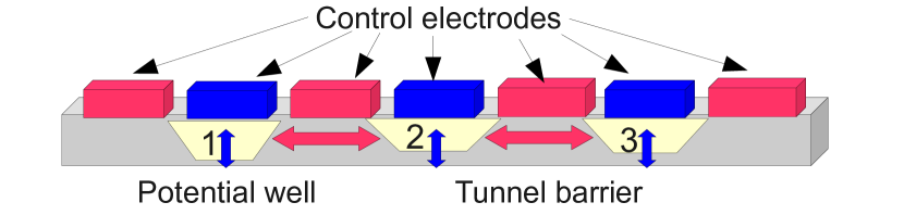
Figure 1: Charged particle trapped in a multi-well potential created by control electrodes. Red electrodes allow control of potential barriers and thus tunnelling rates, while blue electrodes control depths of the wells $1$ to $3$ and thus their energy levels. We can choose default voltage settings such that all wells have the same depth and there is no tunnelling, so that we effectively have $H_{0}=0$. Then by raising or lowering the voltage of electrode $1$ we can introduce a relative phase shift between the ground state $|1\rangle$ of the first well and the other two ground states, and by changing the voltage applied to the red electrode between wells $1$ and $2$ we can induce tunnelling between the first two wells, etc.

3.3 Explicit Control Sequence

To illustrate the constructive procedure, let us consider the case $N=3$ with $Y,Z$ controls. In this case the control operators take the explicit form

$$Z_{2}=\begin{pmatrix}0&0&0\\ 0&1&0\\ 0&0&0\end{pmatrix},\quad Z_{3}=\begin{pmatrix}0&0&0\\ 0&0&0\\ 0&0&1\end{pmatrix},\quad Y_{1}=\begin{pmatrix}0&-i&0\\ i&0&0\\ 0&0&0\end{pmatrix},\quad Y_{2}=\begin{pmatrix}0&0&0\\ 0&0&-i\\ 0&i&0\end{pmatrix}.$$

and the corresponding evolution operators are

$$U_{2}^{Z}(\alpha)=\begin{pmatrix}1&0&0\\ 0&e^{-i\alpha}&0\\ 0&0&1\end{pmatrix},\quad U_{3}^{Z}(\alpha)=\begin{pmatrix}1&0&0\\ 0&1&0\\ 0&0&e^{-i\alpha}\end{pmatrix},$$

$$U_{1}^{Y}(\alpha)=\begin{pmatrix}\cos\alpha&-\sin\alpha&0\\ \sin\alpha&\cos\alpha&0\\ 0&0&1\end{pmatrix},\quad U_{2}^{Y}(\alpha)=\begin{pmatrix}1&0&0\\ 0&\cos\alpha&-\sin\alpha\\ 0&\sin\alpha&\cos\alpha\end{pmatrix},$$

Given these control operators and the hyperspherical coordinate representation of the initial and target states, it is now very easy to see how to steer an arbitrary initial state to an arbitrary target state in the following seven steps:

Step 1. $(\theta^{(0)}_{1},\theta^{(0)}_{2};\phi^{(0)}_{1},\phi^{(0)}_{2})\rightarrow(\theta^{(0)}_{1},\theta^{(0)}_{2};\phi^{(0)}_{1},0)$: Apply phase rotation $U_{3}^{Z}(\phi_{2}^{(0)})$

$$\begin{pmatrix}1&0&0\\ 0&1&0\\ 0&0&e^{-i\phi_{2}^{(0)}}\end{pmatrix}\begin{pmatrix}\cos\theta_{1}^{(0)}\\ e^{i\phi_{1}^{(0)}}\sin\theta_{1}^{(0)}\cos\theta_{2}^{(0)}\\ e^{i\phi_{2}^{(0)}}\sin\theta_{1}^{(0)}\sin\theta_{2}^{(0)}\end{pmatrix}=\begin{pmatrix}\cos\theta_{1}^{(0)}\\ e^{i\phi_{1}^{(0)}}\sin\theta_{1}^{(0)}\cos\theta_{2}^{(0)}\\ \sin\theta_{1}^{(0)}\sin\theta_{2}^{(0)}\end{pmatrix}.$$

Step 2. $(\theta^{(0)}_{1},\theta^{(0)}_{2};\phi^{(0)}_{1},0)\rightarrow(\theta^{(0)}_{1},\theta^{(0)}_{2};0,0)$: Apply phase rotation $U_{2}^{Z}(\phi_{1}^{(0)})$

$$\left(\begin{array}[]{ccc}1&0&0\\ 0&e^{-i\phi_{1}^{(0)}}&0\\ 0&0&1\end{array}\right)\left(\begin{array}[]{c}\cos\theta_{1}^{(0)}\\ e^{i\phi_{1}^{(0)}}\sin\theta_{1}^{(0)}\cos\theta_{2}^{(0)}\\ \sin\theta_{1}^{(0)}\sin\theta_{2}^{(0)}\end{array}\right)=\left(\begin{array}[]{c}\cos\theta_{1}^{(0)}\\ \sin\theta_{1}^{(0)}\cos\theta_{2}^{(0)}\\ \sin\theta_{1}^{(0)}\sin\theta_{2}^{(0)}\end{array}\right)$$

Step 3. $(\theta^{(0)}_{1},\theta^{(0)}_{2};0,0)\rightarrow(\theta^{(0)}_{1},0;0,0)$: Apply population rotation $U_{2}^{Y}(-\theta_{2}^{(0)})$

$$\left(\begin{array}[]{ccc}1&0&0\\ 0&\cos\theta_{2}^{(0)}&\sin\theta_{2}^{(0)}\\ 0&-\sin\theta_{2}^{(0)}&\cos\theta_{2}^{(0)}\end{array}\right)\left(\begin{array}[]{c}\cos\theta_{1}^{(0)}\\ \sin\theta_{1}^{(0)}\cos\theta_{2}^{(0)}\\ \sin\theta_{1}^{(0)}\sin\theta_{2}^{(0)}\end{array}\right)=\left(\begin{array}[]{c}\cos\theta_{1}^{(0)}\\ \sin\theta_{1}^{(0)}\\ 0\end{array}\right)$$

Step 4. $(\theta^{(0)}_{1},0;0,0)\rightarrow(\theta^{(s)}_{1},,0;0,0)$: Apply population rotation $U_{1}^{Y}(\theta_{1}^{(s)}-\theta_{1}^{(0)})$

$$\left(\begin{array}[]{ccc}\cos(\theta_{1}^{(s)}-\theta_{1}^{(0)})&-\sin(\theta_{1}^{(s)}-\theta_{1}^{(0)})&0\\ \sin(\theta_{1}^{(s)}-\theta_{1}^{(0)})&\cos(\theta_{1}^{(s)}-\theta_{1}^{(0)})&0\\ 0&0&1\end{array}\right)\left(\begin{array}[]{c}\cos\theta_{1}^{(0)}\\ \sin\theta_{1}^{(0)}\\ 0\end{array}\right)=\left(\begin{array}[]{c}\cos\theta_{1}^{(s)}\\ \sin\theta_{1}^{(s)}\\ 0\end{array}\right)$$

Step 5. $(\theta^{(s)}_{1},0;0,0)\rightarrow(\theta^{(s)}_{1},\theta^{(s)}_{2};0,0)$: Apply population rotation $U_{2}^{Y}(\theta_{2}^{(s)})$

$$\left(\begin{array}[]{ccc}1&0&0\\ 0&\cos\theta_{2}^{(s)}&-\sin\theta_{2}^{(s)}\\ 0&\sin\theta_{2}^{(s)}&\cos\theta_{2}^{(s)}\end{array}\right)\left(\begin{array}[]{c}\cos\theta_{1}^{(s)}\\ \sin\theta_{1}^{(s)}\\ 0\end{array}\right)=\left(\begin{array}[]{c}\cos\theta_{1}^{(s)}\\ \sin\theta_{1}^{(s)}\cos\theta_{2}^{(s)}\\ \sin\theta_{1}^{(s)}\sin\theta_{2}^{(s)}\end{array}\right)$$

Step 6. $(\theta^{(s)}_{1},\theta^{(s)}_{2};0,0)\rightarrow(\theta^{(s)}_{1},\theta^{(s)}_{2};\phi^{(s)}_{1},0)$: Apply phase rotation $U_{2}^{Z}(-\phi_{1}^{(s)})$

$$\left(\begin{array}[]{ccc}1&0&0\\ 0&e^{i\phi_{1}^{(s)}}&0\\ 0&0&1\end{array}\right)\left(\begin{array}[]{c}\cos\theta_{1}^{(s)}\\ \sin\theta_{1}^{(s)}\cos\theta_{2}^{(s)}\\ \sin\theta_{1}^{(s)}\sin\theta_{2}^{(s)}\end{array}\right)=\left(\begin{array}[]{c}\cos\theta_{1}^{(s)}\\ e^{i\phi_{1}^{(s)}}\sin\theta_{1}^{(s)}\cos\theta_{2}^{(s)}\\ \sin\theta_{1}^{(s)}\sin\theta_{2}^{(s)}\end{array}\right)$$

Step 7. $(\theta^{(s)}_{1},\theta^{(s)}_{2};\phi^{(s)}_{1},0)\rightarrow(\theta^{(s)}_{1},\theta^{(s)}_{2};\phi^{(s)}_{1},\phi^{(s)}_{2})$: Apply phase rotation $U_{3}^{Z}(-\phi_{2}^{(s)})$

$$\left(\begin{array}[]{ccc}1&0&0\\ 0&1&0\\ 0&0&e^{i\phi_{2}^{(s)}}\end{array}\right)\left(\begin{array}[]{c}\cos\theta_{1}^{(s)}\\ e^{i\phi_{1}^{(s)}}\sin\theta_{1}^{(s)}\cos\theta_{2}^{(s)}\\ \sin\theta_{1}^{(s)}\sin\theta_{2}^{(s)}\end{array}\right)=\left(\begin{array}[]{c}\cos\theta_{1}^{(s)}\\ e^{i\phi_{1}^{(s)}}\sin\theta_{1}^{(s)}\cos\theta_{2}^{(s)}\\ e^{i\phi_{2}^{(s)}}\sin\theta_{1}^{(s)}\sin\theta_{2}^{(s)}\end{array}\right)$$

The generalization to $N>3$ is straightforward, as shown in Algorithm 2. Given a Hamiltonian of the form

$$H=\sum_{m=1}^{2N-1}u_{m}(t)H_{m}$$ (10)

where $H_{2n-1}=Z_{n+1}$, $H_{2n}=Y_{n}$ and $u_{m}(t)$ are controls (e.g. voltages), the bang-bang control sequence given by Algorithm 2 can be implemented by applying $4N-5$ control pulses. At the $k$th step we apply a constant control field $u_{S(k)}=L_{k}$ for time $t_{k}=\gamma_{k}/L_{k}$, while all other controls are set to $0$ (or the voltages are set to their default values). Notice that in practice we cannot apply fields for negative times, thus the sign of $L_{k}$ must match that of $\gamma_{k}$. However, if $\gamma_{k}$ is negative and $L_{k}>0$, we can also apply a field $f_{S(k)}=L_{k}$ for time $t_{k}=(\gamma_{k}+2\pi)/L_{k}$ as $\gamma_{k}+2\pi>0$ and effects the same rotation.

If $X_{n}$ control Hamiltonians are used instead of $Y_{n}$ control Hamiltonians, error $i^{n-1}$ is created in the $n$th coordinate by the population rotations. So the algorithm need be slightly modified to correct phase factors of $|n\rangle(n=2,\cdots,N)$. We can achieve this by adding $\tfrac{\pi}{2}(n\mod 4)$ to the phase angles $\phi_{n}$, noting that $e^{i\pi/2(n\mod 4)}=i^{n}$ and the phase factor of the $n$th coordinate is $e^{i\phi_{n-1}}$.

Besides giving explicit expressions for the rotation angles in the decomposition, the scheme has an additional advantage compared the the standard decomposition Eq.(4) considered earlier: While the rotations in the standard factorization do not commute, the first $N-1$ and final $N-1$ phase rotations in the decomposition based on complex hyperspherical coordinates are represented by diagonal matrices which commute. This means that these operations can be applied concurrently rather than sequentially, leading to a potentially considerable reduction in the total length of the control sequence.

($S,\gamma$) $\leftarrow$ StateTransfer ($c^{(0)},c^{(s)}$)
Compute sequence of rotations required for state transfer
In:	$c^{(0)},c^{(s)}$	initial and target state vectors
Out:	$S,\gamma$	Bang-bang control sequence
1 $(\theta^{(0)},\phi^{(0)})$ $\leftarrow$ HyperCoord$(c^{(0)})$ 2 $(\theta^{(s)},\phi^{(s)})$ $\leftarrow$ HyperCoord$(c^{(s)})$ 3 for $n$ $\leftarrow$ $N-1,\ldots,1$ 4 Append $S$ by $2n-1$, $\gamma$ by $\phi_{n}^{(0)}$  // Apply Phase Rotation $U_{n+1}^{Z}(\phi_{n}^{(0)})$ 5 for $n$ $\leftarrow$ $N-1,\ldots,2$ 6 Append $S$ by $2n$, $\gamma$ by $-\theta_{n}^{(0)}$  // Apply Population Rotation $U_{n}^{Y}(-\theta_{n}^{(0)})$ 7 Append $S$ by $2$, $\gamma$ by $\theta_{1}^{(s)}-\theta_{1}^{(0)}$  // Apply Population Rotation $U_{1}^{Y}(\theta_{1}^{(s)}-\theta_{1}^{(0)})$ 8 for $n$ $\leftarrow$ $2,\ldots,N-1$ 9 Append $S$ by $2n$, $\gamma$ by $\theta_{n}^{(s)}$  // Apply Population Rotation $U_{n}^{Y}(\theta_{n}^{(s)})$ 10 for $n$ $\leftarrow$ $1,\ldots,N-1$ 11 Append $S$ by $2n-1$, $\gamma$ by $-\phi_{n}^{(s)}$  // Apply Phase Rotation $U_{n+1}^{Z}(-\phi_{n}^{(s)})$

Algorithm 2: Control Scheme to achieve state transfer $\vec{c}^{(0)}\mapsto\vec{c}^{(s)}$ in $4N-5$ steps using bang-bang control, based on hyperspherical coordinate parametrization. $\vec{S}$ and $\vec{\gamma}$ are vectors of length $4N-5$, whose elements are integer labels indicating the control Hamiltonian ($m=1,\ldots,2N-2$) and rotation angle $\gamma_{k}$, respectively.

3.4 Application: Creating a multi-partite-entangled $W$-state

As a simple application of the scheme, suppose first that we have $N$ sites and starting with only site $1$ populated, i.e., in state $|1\rangle$, we would like to prepare an equal superposition of all $N$ sites $|n\rangle$ for $n=1,\ldots,N$:

$$|\psi\rangle=\tfrac{1}{\sqrt{N}}\sum_{n=1}^{N}|n\rangle.$$

All we need to do is compute the hyperspherical coordinates of $|\psi\rangle$, e.g., for $N=10$

$$\vec{\theta}=(1.2490,1.2310,1.2094,1.1832,1.1503,1.1071,1.0472,0.9553,0.7854)$$

and here clearly $\vec{\varphi}=\vec{0}$, which tells us that we need to apply a sequence of $9$ $Y$-rotations

$$U^{Y}_{9}(\theta_{9})U_{8}^{Y}(\theta_{8})U_{7}^{Y}(\theta_{7})U_{6}^{Y}(\theta_{6})U_{5}^{Y}(\theta_{5})U_{4}^{Y}(\theta_{4})U_{3}^{Y}(\theta_{3})U_{2}^{Y}(\theta_{2})U_{1}^{Y}(\theta_{1})$$

to the initial state $|1\rangle$. This results in the following sequence of states being created

$n=0$	$n=1$	$n=2$	$n=3$	$n=4$	$n=5$	$n=6$	$n=7$	$n=8$	$n=9$
1.0000	0.3162	0.3162	0.3162	0.3162	0.3162	0.3162	0.3162	0.3162	0.3162
0	0.9487	0.3162	0.3162	0.3162	0.3162	0.3162	0.3162	0.3162	0.3162
0	0	0.8944	0.3162	0.3162	0.3162	0.3162	0.3162	0.3162	0.3162
0	0	0	0.8367	0.3162	0.3162	0.3162	0.3162	0.3162	0.3162
0	0	0	0	0.7746	0.3162	0.3162	0.3162	0.3162	0.3162
0	0	0	0	0	0.7071	0.3162	0.3162	0.3162	0.3162
0	0	0	0	0	0	0.6325	0.3162	0.3162	0.3162
0	0	0	0	0	0	0	0.5477	0.3162	0.3162
0	0	0	0	0	0	0	0	0.4472	0.3162
0	0	0	0	0	0	0	0	0	0.3162

Each $Y_{n}$ extends the superposition by one site until we are left with the desired state after the final step. Creating such a superposition state may not seem very interesting but it has an interesting application in the area of entanglement creation, for instance.

The Hamiltonians for many systems such as interacting quantum dots or coupled Josephson junctions, for example, can be described to a reasonably good approximation by an XXZ-spin network model

$$H=\sum_{n}\alpha_{n}\sigma^{Z}_{n}+\sum_{m<n}\gamma_{mn}(\sigma^{X}_{m}\sigma^{X}_{n}+\sigma^{Y}_{m}\sigma^{Y}_{n}+\kappa\sigma^{Z}_{m}\sigma^{Z}_{n}),$$ (11)

where $\sigma^{A}_{n}$ is an $N$-fold tensor product for which the $n$th factor is $A$ and all others are the identity, and $X$, $Y$ and $Z$ are the usual $2\times 2$ Pauli matrices. For a chain with nearest-coupling we have $\gamma_{mn}=0$ except when $n=m+1$ and for $\kappa=0$ we have the so-called XX-coupling model. The Hamiltonian (11) commutes with the total spin operator $S=\sum_{n}Z_{n}$ and decomposes into excitation subspaces for any choice of $\alpha_{n}$ and $\gamma_{mn}$. It is easy to see that a state such as the $W$-state

$$\psi_{W}=\tfrac{1}{\sqrt{N}}\left(|{\uparrow}{\downarrow}{\downarrow}\ldots{\downarrow}\rangle+|{\downarrow}{\uparrow}{\downarrow}\ldots{\downarrow}\rangle+\ldots+|{\downarrow}{\downarrow}\ldots{\downarrow}{\uparrow}\rangle\right)$$ (12)

belongs to the single excitation subspace, as does the state $|{\uparrow}{\downarrow}\ldots{\downarrow}\rangle$. On this subspace the Hamiltonian (11) can be simplified. For a chain with nearest-neighbour coupling and $\kappa=0$ we obtain (up to multiples of the identity):

$$H_{1}=\sum_{n}-\alpha_{n}Z_{n}+\gamma_{n}X_{n},$$ (13)

i.e., the Hamiltonian is exactly of the form required for our scheme. Treating $\alpha_{n}$ and $\gamma_{n}$ as control parameters, we can use the scheme above to create a $W$ state starting from the product state $|1\rangle=|{\uparrow}{\downarrow}\ldots{\downarrow}\rangle$. Since we can only implement $X_{n}$-rotations, we will need to apply the phase corrections

$$\prod_{n=2}^{N}U_{n}^{Z}(\phi_{n}),\quad\phi_{n}=-\tfrac{\pi}{2}(n-1\mod 4),$$

which can be applied concurrently in the final step.

4 Optimal piecewise-constant Control and Time-energy Performance

The bang-bang control sequence given by Algorithm 2 leaves us considerable freedom of choice for the controls. Choosing large control amplitudes will result in short pulse durations, thus optimizing the transfer time $t_{f}$. However, large control amplitudes may not be feasible and have undesirable side effects in terms of transfering too much energy to the system. We can try to optimize the field amplitude by stipulating that the state transfer is to be achieved while minimizing a time-energy performance index

$$J=\int_{0}^{t_{f}}[\lambda+\sum_{m=1}^{2N-2}|u_{m}(t)|^{2}]\,dt$$ (14)

where $\lambda$ is the ratio factor of the costs of time and energy and $\lambda>0$. Larger values of $\lambda$ indicate a stronger emphasis on time-cost, while smaller values of $\lambda$ give more weight to the energy cost of the controls.

If the controls can take values $f_{m}(t)\in\{0,\pm L\}$ and the pulses are applied strictly sequentially, then the total length $t_{f}$ of the control sequence is

$$\begin{split}t_{f}&=\frac{1}{L}\left[\sum_{n=1}^{N-1}|\phi_{n}^{(0)}|+|\phi_{n}^{(s)}|+\sum_{n=2}^{N-1}(\theta_{n}^{(0)}+\theta_{n}^{(s)})+|\theta_{1}^{(s)}-\theta_{1}^{(0)}|\right]\\ &\leq\frac{1}{L}\left[2(N-1)\pi+2(N-2)\frac{\pi}{2}+\frac{\pi}{2}\right]=\frac{(6N-7)\pi}{2L}\end{split}$$ (15)

because of $0\leq\theta_{n}\leq\tfrac{\pi}{2}$ and $0\leq|\phi_{n}|\leq\pi$. Noting that $a^{2}+b^{2}\geq 2ab$, with equality exactly if $a=b$, we have

$$J=\sum_{k=1}^{K}(\lambda+L_{k}^{2})t_{k}\leq\sum_{k=1}^{K}2\sqrt{\lambda}L_{k}t_{k}\leq 2\sqrt{\lambda}t_{f}\max_{k}L_{k}$$ (16)

with equality if and only if $L_{k}=\sqrt{\lambda}$. This shows that the optimal choice of the field amplitudes is $L_{k}=\sqrt{\lambda}$, for which we have

$$t_{f}^{*}\leq\frac{(6N-7)\pi}{2\sqrt{\lambda}},\quad J_{*}=\min J=2\lambda t_{f}^{*}\leq\sqrt{\lambda}(6N-7)\pi$$ (17)

and the corresponding optimal energy cost is $E^{*}=J^{*}-\lambda t_{f}^{*}\leq\frac{1}{2}\sqrt{\lambda}(6N-7)\pi$. As expected, as $\lambda$ goes to $0$, $t_{f}^{*}$ becomes infinite and $E^{*}$ goes to $0$, but their product remains constant

$$\begin{array}[]{c}t_{f}^{*}\cdot{E^{*}}=\left[\sum_{n=1}^{N-1}|\phi_{n}^{(0)}|+|\phi_{n}^{(s)}|+\sum_{n=2}^{N-1}(\theta_{n}^{(0)}+\theta_{n}^{(s)})+|\theta_{1}^{(s)}-\theta_{1}^{(0)}|\right]^{2}\leq\frac{(6N-7)^{2}\pi^{2}}{4}\end{array}$$ (18)

and depends only on the geometric parameters of the initial state and target states.

If first and last $N-1$ phase rotations are applied concurrently the transfer time is reduced

$$\begin{split}t_{f}^{\prime}&=\frac{1}{L}\left[\max_{n}|\phi_{n}^{(0)}|+\max_{n}|\phi_{n}^{(s)}|+\sum_{n=2}^{N-1}(\theta_{n}^{(0)}+\theta_{n}^{(s)})+|\theta_{1}^{(s)}-\theta_{1}^{(0)}|\right]\\ &\leq\frac{1}{L}\left[2\pi+2(N-2)\frac{\pi}{2}+\frac{\pi}{2}\right]=\frac{(2N+3)\pi}{2L}.\end{split}$$ (19)

Setting $\phi_{\max}^{(0)}=\max_{n}|\phi_{n}^{(0)}|$ and $\phi_{\max}^{(s)}=\max_{n}|\phi_{n}^{(s)}|$, shows that we have $t_{1}=\phi_{\max}^{(0)}/L$ and $t_{K}=\phi_{\max}^{(s)}/L$, and thus we must choose $L_{n}\geq\phi_{n}^{(0)}/t_{1}$ and $L_{n}=\phi_{n}^{(s)}/t_{K}$, respectively for the control amplitude of the first and last $N-1$ concurrent pulses to be able to implement all $N-1$ phase rotations concurrently in time $t_{1}$ or $t_{K}$, respectively. Furthermore the performance index changes

$$J\leq 2t_{f}^{\prime}\sqrt{\lambda}\max_{N\leq k\leq K+1-N}L_{k}+\sum_{k=1}^{N-1}L_{k}^{2}+\sum_{k=K-N+2}^{K}L_{k}^{2},$$ (20)

which suggests that we can improve the performance index and reduce the energy cost by choosing the amplitudes of the first and last $N-1$ concurrent pulses to be as small as possible, i.e., $L_{n}=\phi_{n}^{(0)}/t_{1}$ and $L_{n}=\phi_{n}^{(s)}/t_{K}$, and $L_{k}=\sqrt{\lambda}$ for all other amplitudes.

5 Implementation of Unitary Operators

5.1 Complex hyperspherical representation of unitary operators

Any $N-$dimensional unitary operator can be represented as follows:

$$U=\sum_{j=1}^{N}e^{i\varphi_{j}}|u_{j}\rangle\langle u_{j}|$$ (21)

where $\{|u_{j}\rangle\}$ constructs an orthonormal basis set in $N-$dimensional Hilbert space. From (21), we can find that global phase factors of all $|u_{j}\rangle$s do not affect $U$, so they can be neglected. Assuming $\langle 1|u_{j}\rangle$ is real and positive for each $j$, by (5) the complex hyperspherical parametrization for $\{|u_{j}\rangle:j=1,\cdots,N\}$ can be given by

$$\begin{pmatrix}|u_{1}\rangle\\ |u_{2}\rangle\\ \vdots\\ |u_{N}\rangle\end{pmatrix}=\begin{pmatrix}\mathbf{I}_{N-2}&0\\ 0&C^{(2)}\end{pmatrix}\cdots\begin{pmatrix}\mathbf{I}_{1}&0\\ 0&C^{(N-1)}\end{pmatrix}C^{(N)}\begin{pmatrix}|1\rangle\\ |2\rangle\\ \vdots\\ |N\rangle\end{pmatrix}$$ (22)

where

$$C^{(k)}=\left(\overrightarrow{c_{1}}^{(k)}),(\overrightarrow{c_{2}}^{(k)},\ldots,(\overrightarrow{c_{k-1}}^{(k)}),(\overrightarrow{c_{k}}^{(k)})\right)^{T},$$ (23)

and $(\overrightarrow{c_{i}}^{(k)})^{T}$ is the transpose of the vector $\overrightarrow{c_{i}}^{(k)}$ and

$$\overrightarrow{c_{1}}^{(k)} =\begin{pmatrix}\cos\theta_{1}^{(k)}\\ e^{i\phi_{1}^{(k)}}\sin\theta_{1}^{(k)}\cos\theta_{2}^{(k)}\\ \vdots\\ e^{i\phi_{k-2}^{(k)}}\prod_{l=1}^{k-2}\sin\theta_{l}^{(k)}\cos\theta_{k-1}^{(k)}\\ e^{i\phi_{k-1}^{(k)}}\prod_{l=1}^{k-1}\sin\theta_{l}^{(k)}\end{pmatrix},$$ (24)

$$\overrightarrow{c_{2}}^{(k)} =\begin{pmatrix}\sin\theta_{1}^{(k)}\\ -e^{i\phi_{1}^{(k)}}\cos\theta_{1}^{(k)}\cos\theta_{2}^{(k)}\\ \vdots\\ -e^{i\phi_{k-2}^{(k)}}\cos\theta_{1}^{(k)}\prod_{l=2}^{k-2}\sin\theta_{l}^{(k)}\cos\theta_{k-1}^{(k)}\\ -e^{i\phi_{k-1}^{(k)}}\cos\theta_{1}^{(k)}\prod_{l=2}^{k-1}\sin\theta_{l}^{(k)}\end{pmatrix},$$ (25)

and so forth until

$$\overrightarrow{c_{k-1}}^{(k)} =\begin{pmatrix}0\\ \vdots\\ 0\\ e^{i\phi_{k-3}^{(k)}}\sin\theta_{k-2}^{(k)}\\ -e^{i\phi_{k-2}^{(k)}}\cos\theta_{k-2}^{(k)}\cos\theta_{k-1}^{(k)}\\ -e^{i\phi_{k-1}^{(k)}}\cos\theta_{k-2}^{(k)}\sin\theta_{k-1}^{(k)}\end{pmatrix},$$ (26)

$$\overrightarrow{c_{k}}^{(k)} =\begin{pmatrix}0\\ \vdots\\ 0\\ e^{i\phi_{k-2}^{(k)}}\sin\theta_{k-1}^{(k)}\\ -e^{i\phi_{k-1}^{(k)}}\cos\theta_{k-1}^{(k)}\end{pmatrix}$$ (27)

for $2\leq k\leq N$. Note that $C^{(k)}(C^{(k)})^{\dagger}=\mathbf{I}_{k}$.

5.2 Realization of unitary operators

Suppose that $Y_{n}$ and $Z_{n}$ controls as defined in eqs. (6) and (7b) are permitted for $1\leq n\leq N-1$ and $1\leq n\leq N$, respectively. Then $U$ can be realized by a sequence of bang-bang controls

$$U=T^{\dagger}\underline{\left(\prod_{n=1}^{N}U_{n}^{Z}(\varphi_{n})\right)}T$$ (28)

where

$$T=\prod_{n=2}^{N}U_{n},\quad U_{n}=\prod_{j=1}^{n-1}U_{N-n+j}^{Y}(\theta_{j}^{(n)})\underline{\prod_{j=1}^{n-1}U_{N-n+j+1}^{Z}(\phi_{j}^{(n)})}.$$ (29)

The $Z$-phase rotations (underlined) commute and can be applied concurrently. Thus $U_{n}$ can be implemented in $n$ steps and $T$ in $N(N+1)/2-1$ steps and the entire process in $N(N+1)-1$ steps. If we took the more contentional approach of factoring an operator $U\in\mathbf{SU}(N)$ into a sequence of $N(N+1)/2$ rotations on two-level subspaces, e.g., spanned by $\{|n\rangle,|n+1\rangle\}$, and further decomposed each of these $\mathbf{SU}(2)$ rotations into three elementary $Y_{n}$ and $Z_{n}$ rotations using the Euler decomposition, we would require $3N(N+1)/2$ steps instead, and since $Z_{n}$ and $Y_{n}$ operations do not commute, these could not be implemented concurrently.

The proof of the result is constructive.

(1) Effect of each $\mathbf{U_{n}}$. Let $|e^{(n)}\rangle$ be an arbitrary state in the space spanned by $\{|1\rangle,|2\rangle,\cdots,|N-n\rangle\}$ and

$$\begin{pmatrix}|e_{N-n+1}^{(n)}\rangle\\ |e_{N-n+2}^{(n)}\rangle\\ \vdots\\ |e_{N}^{(n)}\rangle\end{pmatrix}=C^{(n)}\begin{pmatrix}|N-n+1\rangle\\ |N-n+2\rangle\\ \vdots\\ |N\rangle\end{pmatrix}$$

where $C^{(n)}$ is as defined in Eq.(23). That is,

$$|e_{N-n+1}^{(n)}\rangle= \cos\theta_{1}^{(n)}|N-n+1\rangle+e^{i\phi_{1}^{(n)}}\sin\theta_{1}^{(n)}\cos\theta_{2}^{(n)}|N-n+2\rangle$$

$$+\cdots+e^{i\phi_{n-2}^{(n)}}\sin\theta_{1}^{(n)}\cdots\sin\theta_{n-2}^{(n)}\cos\theta_{n-1}^{(n)}|N-1\rangle$$

$$+e^{i\phi_{n-1}^{(n)}}\sin\theta_{1}^{(n)}\cdots\sin\theta_{n-2}^{(n)}\sin\theta_{n-1}^{(n)}|N\rangle$$

$$|e_{N-n+2}^{(n)}\rangle= \sin\theta_{1}^{(n)}|N-n+1\rangle-e^{i\phi_{1}^{(n)}}\cos\theta_{1}^{(n)}\cos\theta_{2}^{(n)}|N-n+2\rangle$$

$$-\cdots-e^{i\phi_{n-2}^{(n)}}\cos\theta_{1}^{(n)}\sin\theta_{2}^{(n)}\cdots\sin\theta_{n-2}^{(n)}\cos\theta_{n-1}^{(n)}|N-1\rangle$$

$$-e^{i\phi_{n-1}^{(n)}}\cos\theta_{1}^{(n)}\sin\theta_{2}^{(n)}\cdots\sin\theta_{n-2}^{(n)}\sin\theta_{n-1}^{(n)}|N\rangle$$

$$\cdots\cdots$$

$$|e_{N-1}^{(n)}\rangle= e^{i\phi_{n-3}^{(n)}}\sin\theta_{n-2}^{(n)}|N-2\rangle$$

$$-e^{i\phi_{n-2}^{(n)}}\cos\theta_{n-2}^{(n)}\cos\theta_{n-1}^{(n)}|N-1\rangle-e^{i\phi_{n-1}^{(n)}}\cos\theta_{n-2}^{(n)}\sin\theta_{n-1}^{(n)}|N\rangle$$

$$|e_{N}^{(n)}\rangle= e^{i\phi_{n-2}^{(n)}}\sin\theta_{n-1}^{(n)}|N-1\rangle-e^{i\phi_{n-1}^{(n)}}\cos\theta_{n-1}^{(n)}|N\rangle.$$

$U_{n}$ leaves any state $|e^{(n)}\rangle$ in the subspace spanned by $\{|1\rangle,|2\rangle,\cdots,|N-n\rangle\}$ invariant, i.e., $U_{n}|e^{(n)}\rangle=|e^{(n)}\rangle$ as $U_{n}$ is the identity on this subspace. Furthermore, Sec. 3.3 shows that applying $U_{n}$ to $|e_{N-n+1}\rangle$ maps it to the basis state $|N-n+1\rangle$, and we can verify by direct computation

$$U_{n}|e_{N-n+2}^{(n)}\rangle =U_{N-n+1}^{Y}(\theta_{1}^{(n)})(\sin\theta_{1}^{(n)}|N-n+1\rangle-\cos\theta_{1}^{(n)}|N-n+2\rangle)$$

$$=-|N-n+2\rangle$$

$$\cdots\cdots$$

$$U_{n}|e_{N-1}^{(n)}\rangle =\prod_{j=1}^{n-2}U_{N-n+j}^{Y}(\theta_{j}^{(n)})(\sin\theta_{n-2}^{(n)}|N-2\rangle-\cos\theta_{n-2}^{(n)}|N-1\rangle)$$

$$=-|N-1\rangle$$

$$U_{n}|e_{N}^{(n)}\rangle =\prod_{j=1}^{n-1}U_{N-n+j}^{Y}(\theta_{j}^{(n)})(\sin\theta_{n-1}^{(n)}|N-1\rangle-\cos\theta_{n-1}^{(n)}|N-2\rangle)$$

$$=-|N\rangle$$

$$\begin{cases}\begin{array}[]{ll}U_{n}|e^{(n)}\rangle=|e^{(n)}\rangle&|e^{(n)}\rangle\in\mbox{\rm Span}\{|1\rangle,\cdots,|N-n\rangle\}\\ U_{n}|e_{N-n+1}^{(n)}\rangle=|N-n+1\rangle\\ U_{n}|e_{j}^{(n)}\rangle=-|j\rangle&N-n+2\leq j\leq N.\end{array}\end{cases}$$ (30)

(2) Effect of $\mathbf{T}$. Using the previous result we now show that $T|u_{n}\rangle=(-1)^{(n-1)}|n\rangle$ with $|u_{n}\rangle$ as defined in (22). Let $\vec{a}^{(k)}=(0,\cdots,0,(\overrightarrow{c_{1}}^{(k)})^{T})$ be a row vector of length $N$ where the coefficient vector $c_{1}^{(k)}$ is as in Eq. (24) and the number of zeros is $N-k$. Eqs (22)–(29) and (30) give

$$T|u_{1}\rangle =U_{1}\cdots U_{N}\vec{a}^{(N)}\begin{pmatrix}|1\rangle\\ \vdots\\ |N\rangle\end{pmatrix}$$

$$=U_{1}\cdots U_{N-1}U_{N}|e_{1}^{(N)}\rangle=U_{1}\cdots U_{N-1}|1\rangle=|1\rangle$$

$$T|u_{2}\rangle =U_{1}\cdots U_{N}\vec{a}^{(N-1)}C^{(N)}\begin{pmatrix}|1\rangle\\ \vdots\\ |N\rangle\end{pmatrix}=U_{1}\cdots U_{N}\vec{a}^{(N-1)}\begin{pmatrix}|e_{1}^{(N)}\rangle\\ \vdots\\ |e_{N}^{(N)}\rangle\end{pmatrix}$$

$$=U_{1}\cdots U_{N-1}\vec{a}^{(N-1)}\begin{pmatrix}|1\rangle\\ -|2\rangle\\ \vdots\\ -|N\rangle\end{pmatrix}=-U_{1}\cdots U_{N-1}|e_{2}^{(N-1)}\rangle=-|2\rangle$$

Furthermore, for $3\leq n\leq N-1$ we have

$$U_{N}|u_{n}\rangle= \vec{a}^{(N-n+1)}\prod_{k=N-n+2}^{N-1}\begin{pmatrix}\mathbf{I}_{N-k}&\\ &C^{(k)}\end{pmatrix}\begin{pmatrix}|1\rangle\\ -|2\rangle\\ \vdots\\ -|N\rangle\end{pmatrix}$$

$$= \vec{a}^{(N-n+1)}\prod_{k=N-n+2}^{N-2}\begin{pmatrix}\mathbf{I}_{N-k}&\\ &C^{(k)}\end{pmatrix}\begin{pmatrix}|1\rangle\\ -|e_{2}^{(N-1)}\rangle\\ \vdots\\ -|e_{N}^{(N-1)}\rangle\end{pmatrix}$$

$$U_{N-1}U_{N}|u_{n}\rangle= \vec{a}^{(N-n+1)}\prod_{k=N-n+2}^{N-3}\begin{pmatrix}\mathbf{I}_{N-k}&\\ &C^{(k)}\end{pmatrix}\begin{pmatrix}|1\rangle\\ -|2\rangle\\ (-1)^{2}|e_{3}^{(N-2)}\rangle\\ \vdots\\ (-1)^{2}|e_{N}^{(N-2)}\rangle\end{pmatrix}$$

and continuing we obtain for $3\leq n\leq N-1$

$$U_{N-n+3}\cdots U_{N}|u_{n}\rangle= \vec{a}^{(N-n+1)}\begin{pmatrix}(-1)^{0}|1\rangle\\ \vdots\\ (-1)^{(n-3)}|n-2\rangle\\ (-1)^{(n-2)}|e_{n-1}^{(N-n+2)}\rangle\\ \vdots\\ (-1)^{(n-2)}|e_{N}^{(N-n+2)}\rangle\end{pmatrix}$$

$$U_{N-n+2}\cdots U_{N}|u_{n}\rangle= (-1)^{(n-1)}|e_{n}^{(N-n+1)}\rangle$$

$$T|u_{n}\rangle=U_{N-n+1}\cdots U_{N}|u_{n}\rangle= (-1)^{(n-1)}|n\rangle,$$

Finally, we have

$$U_{3}\cdots U_{N}\prod_{k=3}^{N-2}\begin{pmatrix}\mathbf{I}_{N-k}&\\ &C^{(k)}\end{pmatrix}C^{(N)}\begin{pmatrix}|1\rangle\\ |2\rangle\\ \vdots\\ |N\rangle\end{pmatrix}=\begin{pmatrix}(-1)^{0}|1\rangle\\ \vdots\\ (-1)^{(N-2)}|N-1\rangle\rangle\\ (-1)^{(N-2)}|N\rangle\end{pmatrix}$$

and thus

$$T|u_{N}\rangle= U_{2}(0,\cdots,0,(\overrightarrow{c_{2}}^{(2)})^{T})\begin{pmatrix}(-1)^{0}|1\rangle\\ \vdots\\ (-1)^{(N-2)}|N-1\rangle\\ (-1)^{(N-2)}|N\rangle\end{pmatrix}$$

$$= U_{2}(-1)^{(N-2)}|e_{N}^{(2)}\rangle=(-1)^{(N-1)}|N\rangle.$$

Thus we finally have

$$TUT^{\dagger}=\sum_{n=1}^{N}e^{i\varphi_{n}}T|u_{n}\rangle\langle u_{n}|T^{\dagger}=\sum_{n=1}^{N}e^{i\varphi_{n}}|n\rangle\langle n|=\prod_{n=1}^{N}U_{n}^{Z}(\varphi_{n})$$

and $U=T^{\dagger}\prod_{n=1}^{N}U_{n}^{Z}(\varphi_{n})T$ as claimed.

6 Discussions and Conclusion

We have presented an explicit geometric control scheme for quantum state transfer problems based on a parametrization of the pure state vectors in terms of complex hyperspherical coordinates. Although it is not difficult to find constructive control schemes for state transfer based on Lie group decompositions, most schemes do not give explicit expressions for the rotation angles (“generalized Euler angles”) in the factorization, and thus the rotation angles usually have to computed numerically. By parametrizing the initial and target states in terms of hyperspherical coordinates, we obtain a factorization where all generalized Euler angles are given explicitly in terms of the hyperspherical coordinates of the initial and target states, eliminating the need for numerical calculation of the generalized Euler angles, aside from computation of the hyperspherical coordinates, which is trivial in terms of computational overhead.

The factorization is applicable given controls capable of implementing phase rotations and population rotations (of either $X$ or $Y$ type) on a collection of two-dimensional subspaces, similar to the general requirements for constructive geometric control schemes. Compared to control schemes based on the standard factorization, this scheme has the additional advantages that all initial and final phase rotations can be combined in a single step and executed concurrently, reducing the time required to achieve the state transfer. As with all bang-bang control schemes based on Lie group decompositions, the factorization only determines the sequence in which the controls are applied and the pulse area (rotation angle) of the control pulses, leaving us with considerable freedom to choose the pulse shapes and amplitudes, which can be used to further optimize a performance index. Here we have considered optimization of the pulse amplitudes for piecewise constant controls such as to minimize a time-energy performance index that takes into account the competing goals of trying to minimize the transfer time and energy cost of the controls.

The scheme can be generalized to realize unitary operators. By expressing the eigenvectors of the target gate $U$ in hyperspherical coordianates we obtain an explicit decomposition for arbitrary unitary operators. Aside from giving explicit expressions for the Euler angles in terms of hyperspherical coordinates an advantage of the decomposition is that it separates the elementary rotations in such a way as to allow concurrent implementation of subsets of operations, which can reduce the control time. Specifially, unlike in many standard decomposition schemes, the $Z_{n}$ and $Y_{n}$ rotations do not occur in an alternating sequence but are clustered. Since the $Z_{n}$ rotations are mutually commuting, this allows concurrent implementation of many operations.

References

References

• [1] H. Rabitz, R. de Vivie-Riedle, M. Motzkus, K. Kompa, Whither the Future of Controlling Quantum Phenomena? Science 288 (2000) 824-828.
• [2] M. A. Nielsen, I. L. Chuang, Quantum Computation and Quantum Information, Cambridge, Cambridge University Press 2000.
• [3] G. M. Huang, T. J. Tarn, J. W. Clark, On the Controllability of Quantum Mechanical Systems, J. Math. Phys. 24 (1983) 2608-2618,.
• [4] C. K. Ong, G. Huang, T. J. Tarn, J. W. Clark, Invertibility of Quantum Mechanical Control Systems, Math. Sys. Theor. 17 (1984) 335-350.
• [5] J. W. Clark, C. Ong, T. J. Tarn, G. M. Huang, Quantum non-Demolition Filters, Math. Sys. Theor. 18 (1985) 33-53.
• [6] A. Blaquiere, S. Diner, G. Lochak, (edit) Information Complexity and Control in Quantum Physics, Springer-Verlag, New York, 1987.
• [7] A. P. Peirce, M. A. Dahleh, H. Rabitz, Optimal control of quantum-mechanical systems: Existence, numerical approximation, and applications, Phys. Rev. A 37 (1988) 4950-4964.
• [8] D. D’Alessandro, Introduction to quantum control and dynamics, CRC Press, 2007.
• [9] H. M. Wiseman, G. J. Milburn, Quantum Measurement and Control, Cambridge University Press, Cambridge, 2010.
• [10] J. Janszky, P. Domokos, S. Szabó, P. Adam, Quantum-state engineering via discrete coherent-state superpositions, Phys. Rev. A 51 (1995) 4191–4193.
• [11] Y. Makhlin, G. Schön, A. Shnirman, Quantum-state engineering with Josephson-junction devices, Rev. Mod. Phys. 73 (2001) 357-400.
• [12] C. Rangan, A. M. Bloch, C.Monroe, P. H. Bucksbaum, Control of Trapped-Ion Quantum States with Optical Pulses, Phys. Rev. Lett. 92 (2004) 113004.
• [13] D. C. Brody and D. W. Hook, On optimum Hamiltonians for state transformations J. Phys. A: Math. Gen. 39 167–170 (2006); ibid. 2007, 40 10949.
• [14] S.Y. Lee, H. Nha, Quantum state engineering by a coherent superposition of photon subtraction and addition, Phys. Rev. A 82 (2010) 053812.
• [15] A. C. Doherty, K. Jacobs, Feedback control of quantum systems using continuous state estimation, Phys. Rev. A 60 (1999) 2700-2711.
• [16] R. van Handel, J. K. Stockton, H. Mabuchi, Feedback control of quantum state reduction, IEEE Trans. Automat. Contr. 50 (2005) 768-780.
• [17] N. Yamamoto, K. Tsumura, S. Hara , Feedback control of quantum entanglement in a two-spin system, Automatica 43 (2007) 981-992.
• [18] S. G. Schirmer, X. Wang, Stabilizing open quantum system by Markovian reservoir engineering, Phys. Rev. A 81 (2010) 062306
• [19] F. Ticozzi, S. G. Schirmer, X. Wang, Stabilizing generic quantum states with Markovian Dynamical Semigroups, IEEE Trans. Autom. Control 55(12) (2010) 2901–2905
• [20] J. Zhang, R.-B. Wu, C.-W. Li, T.-J. Tarn, Protecting coherence and entanglement by quantum feedback controls, IEEE Trans. Automat. Contr. 53 (2010) 619-633.
• [21] X. Wang, A. Bayat, S. Bose and S. G. Schirmer, Global Control Methods for GHZ State Generation on a 1D Ising Chain, Phys. Rev. A 82 (2010) 012330.
• [22] X. Wang, A. Bayat, S. G. Schirmer, S. Bose, Robust Entanglement in Anti-ferromagnetic Heisenberg Chains by Single-spin Optimal Control, Phys. Rev. A81 (2010) 032312
• [23] M. Reck, A. Zeilinger, H. J. Bernstein, P. Bertani, Experimental realization of any discrete unitary operator, Phys. Rev. Lett. 73 (1994) 58-61.
• [24] V. Ramakrishna, K.L. Flores, H. Rabitz, R. J. Ober, Control of a coupled two-spin system without hard pulses, Phys. Rev. A 62 (2000) 053409.
• [25] D. D’Alessandro, The optimal control problem on SO(4) and its applications to quantum control, IEEE Trans. Automat. Contr. 47 (2002) 87-92.
• [26] S. G. Schirmer, A. D. Greentree, V. Ramakrishna, and H. Rabitz, Constructive control of quantum systems using factorization of unitary operators, J. Phys. A 35 (2002) 8315-8339.
• [27] R. Cabrera, T. Strohecker, and H. Rabitz, The canonical coset decomposition of unitary matrices through Householder transformations, J. Math. Phys. 51 (2010) 082101.
• [28] R. Romano, D. D’Alessandro, Environment-Mediated Control of a Quantum System, Phys. Rev. Lett. 97 (2006) 080402.
• [29] M. Zhang, H. Y. Dai, X. C. Zhu, X. W. Li, and D. Hu, Control of the quantum open system by quantum generalized measurement Phys. Rev. A 73 (2006) 032101.
• [30] X. Wang, S. G. Schirmer, Arbitrarily-high steady-state entanglement between non-interacting atoms via collective decay and adiabatic control (2010), arXiv:1005.2114
• [31] H. M. Wiseman, G. J. Milburn, Squeezing via feedback, Phys. Rev. A 49 (1994) 1350-1366.
• [32] M. Yanagisawa, H. Kimura, Transfer Function Approach to Quantum Control-Part I: Dynamics of Quantum Feedback Systems, IEEE Trans. Automat. Contr. 48 (2003) 2107-2120.
• [33] M. Mirrahimi, P. Rouchon, G. Turinici, Lyapunov control of bilinear Schrodinger equations, Automatica 41 (2005) 1987-1994.
• [34] M. R. Jovanovic and B. Bamieh, Lyapunov-based distributed control of systems on lattices, IEEE Trans. Automat. Contr. 50 (2005) 422-433.
• [35] C. Altafini, Feedback stabilization of isospectral control systems on complex flag manifolds: Application to quantum ensembles, IEEE Trans. Automat. Contr. 52 (2007) 2019-2028.
• [36] S. Kuang, S. Cong, Lyapunov control methods of closed quantum systems, Automatica 44 (2008) 98-108.
• [37] X. Wang, S. G. Schirmer, Entanglement generations between distant atoms by Lyapunov Control, Phys. Rev. A 80 (2009) 042305.
• [38] X. Wang, S. G. Schirmer, Analysis of Lyapunov method for control of quantum states, IEEE Trans. Atom. Control 55 (2010) 2259-2270; Analysis of Effectiveness of Lyapunov Control for Non-generic Quantum States, IEEE Trans. Autom. Control 55 (2010), 1406-1411.
• [39] Shai Machnes, U. Sander, S. J. Glaser, P. de Fouquieres, S. G. Schirmer, T. Schulte-Herbruggen, A Unified Programming Platform for Optimising and Benchmarking Quantum Control Algorithms (2010) arXiv:1011.4874.
• [40] D. J. Maas, D. I. Duncan, R. B. Vrijen, W. J. van der Zande, and L. D. Noordam, Vibrational ladder climbing in NO by (sub)picosecond frequency-chirped infrared laser pulses, Chem. Phys. Lett. 290 (1998) 75–80.
• [41] N. Khaneja, R.Brockett, S. J. Glaser, Time optimal control in spin systems, Phys. Rev. A 63 (2001) 032308.
• [42] L. M. K. Vandersypen and I. L. Chuang, NMR Techniques for quantum control and computation, Rev. Mod. Phys. 76 (2004) 1037
• [43] N. Motee, A. Jadbabaie, Optimal Control of Spatially Distributed Systems, IEEE Trans. Automat. Contr. 53 (2008) 1616-1629.
• [44] F. Ticozzi, A. Ferrante, M. Pavon, Robust steering of n-level quantum systems, IEEE Trans. Automat. Contr. 49 (2004) 1742-1745.
• [45] S. G. Schirmer, Implementation of quantum gates via optimal control, J. Mod. Opt. 56 (2009), 831.
• [46] R. Nigmatullin, S. G. Schirmer, Implementation of Logic Gates on Encoded Qubits via Optimal Control, New J. Phys. 11 (2009) 105032.
• [47] S. G. Schirmer and P. J. Pemberton-Ross, Fast high-fidelity information transfer in spin chain quantum wires, Phys. Rev. A 80, 030301 (2009)
• [48] D. D’Alessandro, Optimal evaluation of generalized Euler angles with applications to control, Automatica 40 (2004) 1997-2002.
• [49] K. Ch. Chatzisavvas, C. Daskaloyannis, C. P. Panos and S. G. Schirmer, Explicit algorithm for generalized Euler angle decomposition of SU(2), Phys. Rev. A 80 (2009), 052329.
• [50] I. Bengtsson, K. Zyczkowski, Geometry of Quantum States: An Introduction to Quantum Entanglement, Cambridge, Cambridge University Press, 2006.
• [51] M. A. Nielsen, M. R. Dowling, M. Gu, A. C. Doherty, Quantum Computation as Geometry, Science 311 (2006) 1133.
• [52] M. Zhang, H. Y. Dai, H. W. Xie, D. Hu, Controllability of multiple qubit systems, Eur. Phys. J. D 45 (2007) 331-334.