The Flux-Flux Correlation Function for Anharmonic Barriers

Abstract

The flux-flux correlation function formalism is a standard and widely used approach for the computation of reaction rates. In this paper we introduce a method to compute the classical and quantum flux-flux correlation functions for anharmonic barriers essentially analytically through the use of the classical and quantum normal forms. In the quantum case we show that the quantum normal form reduces the computation of the flux-flux correlation function to that of an effective one dimensional anharmonic barrier. The example of the computation of the quantum flux-flux correlation function for a fourth order anharmonic barrier is worked out in detail, and we present an analytical expression for the quantum mechanical microcanonical flux-flux correlation function. We then give a discussion of the short-time and harmonic limits.

I Introduction

In spite of the tremendous increase in computer power over the last decades, the computation of quantum reaction rates still is a formidable task. This is the topic of this paper, and we begin by giving the setting that is relevant to our work.

The microcanonical rate constant is given by

$$k(E)=\big{(}2\pi\hbar\rho_{\text{r}}(E)\big{)}^{-1}N(E)\,,$$ (1)

where $\rho_{\text{r}}(E)$ is the density of states of reactants and $N(E)$ is the cumulative reaction probability, which in turn can be formally expressed in terms of the ${\bf S}$ matrix as

$$N(E)=\sum_{J}(2J+1)\sum_{n_{\text{p}},n_{\text{r}}}|S_{n_{\text{p}},n_{\text{r}}}(E,J)|^{2}\,.$$ (2)

Here the inner sum runs over the asymptotic states of reactants and products which are labeled by $n_{\text{r}}$ and $n_{\text{p}}$, respectively, and the outer sum covers all values of total angular momentum $J$.

Though formally correct, the computation of a reaction rate via the ${\bf S}$ matrix is extremely inefficient since the computationally expensive information related to the state-to-state reactivities embodied in the ${\bf S}$ matrix is ”thrown away” as a consequence of the averaging embodied in the summations in (2). Motivated by the success of transition state theory (TST) for computing reaction rates using classical mechanics, many researchers have sought a quantum mechanical version of transition state theory. Recall that the main idea of TST as invented by Eyring, Polanyi and Wigner in the 1930s is to compute classical reaction rates from the flux through a dividing surface in phase space which separates the phase space region associated with reactants from the phase space region associated with products. Assuming the dividing surface to be given by an equation $s({\bf z})=0$, where $s$ is a scalar function on the $2f$-dimensional phase space with coordinates ${\bf z}=({\bf q},{\bf p})=(q_{1},\ldots,q_{f},p_{1},\ldots,p_{f})$ with $s({\bf z})<0$ in the reactants region and $s({\bf z})>0$ in the products region, the classical microcanonical rate constant can be written as

$$k_{\text{CL}}(E)=\rho_{\text{r}}(E)^{-1}(2\pi\hbar)^{-f}\int\mathrm{d}{\bf z}\>\delta(E-H({\bf z}))F({\bf z})\,.$$ (3)

Here $F({\bf z})$ is the so called flux factor which is given by

$$F({\bf z})=\frac{d}{dt}\Theta\big{(}s({\bf z}_{t})\big{)}\bigg{|}_{t=0}=-\{H,\Theta(s)\}({\bf z})$$ (4)

with $\Theta$ denoting the Heaviside function, $\{\cdot,\cdot\}$ denoting the Poisson bracket and ${\bf z}_{t}$ denoting the solution of Hamilton’s equations at time $t$ with initial conditions ${\bf z}_{0}={\bf z}$, i.e. ${\bf z}_{t}=\Phi^{t}_{H}({\bf z})$, where $\Phi_{H}$ is the Hamiltonian flow which acts on ${\bf z}$ for time $t$.

For the TST computation of the rate constant to be useful the dividing surface needs to have the property that it is crossed exactly once by reactive trajectories (i.e. trajectories evolving from reactants to products) and not crossed at all by nonreactive trajectories. A dividing surface not satisfying this no-recrossing property leads to an overestimation of the reaction rate. The construction of a recrossing free dividing surface has posed a major problem in the development of TST. Formally, recrossing trajectories are eliminated by multiplying the integrand in (3) by the projection function

$$P_{\text{r}}({\bf z})=\lim_{t\to+\infty}\Theta\big{(}s({\bf z}_{t})\big{)}$$ (5)

which evaluates to $1$ if the trajectory ${\bf z}_{t}=\Phi^{t}_{H}({\bf z})$ evolves to products for $t\to+\infty$, and to 0 otherwise. It is then not difficult to see that the this way corrected expression for the rate constant can be written in the form

$$k_{\text{CL}}(E)=\big{(}2\rho_{\text{r}}(E)\big{)}^{-1}\int_{-\infty}^{\infty}\mathrm{d}t\,{\mathcal{C}_{\text{CL}}}(E,t)\,,$$ (6)

where ${\mathcal{C}_{\text{CL}}}(E,t)$ is the flux-flux correlation function (FFCF)

$${\mathcal{C}_{\text{CL}}}(E,t)=(2\pi\hbar)^{-f}\int\mathrm{d}{\bf z}\>\delta\big{(}E-H({\bf z})\big{)}F({\bf z})F({\bf z}_{t})\,.$$ (7)

The canonical analogues of the microcanonical expression above are easily obtained from replacing the density of states $\delta(E-H({\bf z}))$ by its canonical counterpart $\exp(-\beta H({\bf z}))$ ($\beta=(k_{\text{B}}T)^{-1}$ denoting the inverse temperature). Miller, Schwartz and Tromp Miller et al. (1983) and Yamamoto Yamamoto (1960) took this as a starting point to express the quantum mechanical rate constant in a similar fashion. For the microcanonical case, this amounts to replacing the phase space functions above by the corresponding operators and the integrals over phase space by the traces of operators. For the quantum analogue of the rate constant in (3), this leads to

$$k_{\text{QM}}(E)=\rho_{\text{r}}(E)^{-1}{\mathrm{Tr}}\left\{\delta(E-\hat{H})\hat{F}\hat{P}_{\text{r}}\right\}\,,$$ (8)

where $\rho_{\text{r}}(E)$ now is the quantum mechanical partition function of the reactants (for which we use the same symbol as in the classical case), the flux factor (4) becomes the operator

$$\hat{F}=\frac{d}{dt}\left(e^{i\hat{H}t/\hbar}\Theta(\hat{s})e^{-i\hat{H}t/\hbar}\right)\bigg{|}_{t=0}=\frac{i}{\hbar}\big{[}\hat{H},\Theta(\hat{s})\big{]}$$ (9)

and the projection function (5) becomes the operator

$$\hat{P}_{\text{r}}=\lim_{t\rightarrow+\infty}\mathrm{e}^{\mathrm{i}\hat{H}t/\hbar}\Theta(\hat{s})\mathrm{e}^{-\mathrm{i}\hat{H}t/\hbar}\,.$$ (10)

Similarly to the classical case expression (8) for the quantum rate constant can then also be rewritten in terms of a flux-flux correlation function, namely

$$k_{\text{QM}}(E)=\big{(}2\rho_{\text{r}}(E)\big{)}^{-1}\int_{-\infty}^{\infty}\mathrm{d}t\,{\mathcal{C}_{\text{QM}}}(E,t)$$ (11)

with

$${\mathcal{C}_{\text{QM}}}(E,t)={\mathrm{Tr}}\left\{\delta(E-\hat{H})\hat{F}e^{i\hat{H}t/\hbar}\hat{F}e^{-i\hat{H}t/\hbar}\right\}\,.$$ (12)

Clearly, the ability to compute the quantum mechanical flux-flux correlation function is essential for computing quantum mechanical reaction rates using this approach. Exact expressions for the canonical quantum mechanical flux-flux correlation function can be found in Miller et al. (1983) for the free particle and in Miller (1974); Miller et al. (1983); Wang et al. (1998) for the one degree-of-freedom (quadratic) parabolic barrier. Calculations for other one degree-of-freedom systems have also been carried out numerically. In particular, the quantum mechanical flux-flux correlation functions for the symmetric and asymmetric Eckart and the double-well potential have been studied in detail (see Ceotto et al. (2005); Venkataraman and Miller (2007)). However, these computations were no ab initio computations leading to analytical expressions, but were carried out using various computational techniques. Indeed, the development of computational techniques to compute the quantum mechanical flux-flux correlation function has been a subject of great interest since the development of this approach.

The traditional approach of quantum mechanics involves basis function techniques, and a review of this approach is given in Miller (1998, 1998). While this particular computational approach has proven successful for “moderately” sized molecules, difficulties are encountered when “large” systems (such as biomolecules) are considered. The obstacle has been termed the“exponential wall” of difficulty that one encounters when attempting to perform numerical quantum calculations in the traditional manner for many degree of freedom systems Department of Energy (2007). Semiclassical methods provide an alternative approach. They have been pioneered by Miller and provide significant computational advantages for “large” systems; see Miller (2008) for a recent review.

In this paper we present a third approach based on recent work on the phase space approach to quantum mechanics that relies heavily on the dynamical systems framework arising from the application of classical and quantum normal form theory. Classically, this approach has provided a way of constructing a recrossing free dividing surface in the neighborhood of a saddle type equilibrium point which forms the barrier between reactants and products (more precisely the existence of the recrossing free dividing surface is guaranteed for energies not too far away from the energy of the saddle) Wiggins et al. (2001); Uzer et al. (2002); Waalkens et al. (2004); Waalkens and Wiggins (2004). The dividing surface at a given energy is bounded by a so called normally hyperbolic invariant manifold (NHIM) Wiggins (1994) which as an invariant subsystem with the given energy forms a ’supermolecule’ localized between reactants and products which can be viewed as the transition state that gave TST its name. The dividing surface and the NHIM can be constructed in an algorithmic fashion based on a classical normal form (CNF) which can be computed in the neighborhood of the saddle. This is a nonlinear canonical transformation of the phase space coordinates which, to any desired order, decouples the dynamics near the saddle into a single reactive mode and bath modes. (Note: the “decoupling” occurs through a local integrable approximation valid in a neighborhood of the saddle, and does in general not imply separability.) More recently it has been shown that the classical construction can be generalized to the quantum case Schubert et al. (2006); Waalkens et al. (2008); Goussev et al. . This essentially involves a systematic quantization of the canonical transformation leading to the decoupling in the classical case. The result is a so called quantum normal form (QNF) which leads to a local decoupling also of the quantum dynamics into a reactive mode and bath modes.

The main objective of this paper is to use the classical and quantum normal forms to analytically compute the classical and quantum FFCFs for anharmonic barriers. The outline is as follows. In Sec. II we describe how the classical and quantum normal forms can be used to express the classical and quantum mechanical FFCFs. Sec. II A is concerned with the classical case, and we show how the dividing surface having the no-recrossing property obtained from classical normal form theory enables a computation of the FFCF that does not require the computation of trajectories. Sec. II B is concerned with the quantum case and we show how the quantum normal form approach enables a reduction of the computation of the FFCF in the general $f$ degree-of-freedom case to the case of a one degree-of-freedom anharmonic barrier. Then in Sec. III we work out in detail the microcanonical quantum FFCF for the example of a barrier in one dimension described by a fourth order anharmonic barrier.

By itself this result should be of some interest because it is the first explicit example of an exact calculation of the FFCF for an anharmonic potential. In Sec. IV we give a discussion of our results and an outlook for future work. The technicalities of two computations are deferred to appendices.

II The flux-flux correlation function in the framework of classical and quantum normal form theory

We begin by showing how classical and quantum normal form theory can be used to calculate both the classical and quantum ${\mathrm{FFCF}}$ for reactions associated with barrier given by an index one saddle of the potential energy surface. In fact the (slightly more general) starting point is an equilibrium point of Hamilton’s equations which is of saddle-center-….-center stability type. For a system with $f$ degrees-of-freedom, this means that the matrix associated with the linearization of Hamilton’s equations about the equilibrium point has one pair of real eigenvalues $\pm\lambda$ and $f-1$ complex conjugate pairs of imaginary eigenvalues $\pm\mathrm{i}\omega_{k}$, $k=2,\ldots,f$. We will call such an equilibrium point a saddle for short. For simplicity, we will restrict ourselves to the generic situation where the linear frequencies $\omega_{k}$ are not resonant, i.e. $m_{2}\omega_{1}+\ldots+m_{f}\omega_{f}\neq 0$ for every nonzero vector of integers $(m_{2},\ldots,m_{f})$.

II.1 The classical case

Classical normal form (CNF) theory Uzer et al. (2002); Waalkens et al. (2008); Goussev et al. provides an algorithm for constructing a (nonlinear) canonical transformation ${\bf z}\mapsto{\bf Z}=(Q_{1},\ldots,Q_{f},P_{1},\ldots,P_{f})$ which, after truncation at a suitable order $N$, leads to an integrable approximation of the dynamics near the saddle. In terms of the normal form coordinates ${\bf Z}$ the $N$th order CNF of the original Hamilton function $H({\bf z})$ assumes the following form

$$\begin{split}H_{\mathrm{CNF}}^{(N)}({\bf Z})&=K_{\mathrm{CNF}}^{(N)}(I,J_{2},J_{3},\ldots,J_{f})\\ &=\sum_{n=0}^{\lfloor N/2\rfloor}\!\sum_{|\alpha|=n}\kappa_{n,\alpha}I^{\alpha_{1}}J_{2}^{\alpha_{2}}\ldots J_{f}^{\alpha_{f}}.\end{split}$$ (13)

Here $\lfloor\cdot\rfloor$ denotes the floor function, the $\alpha=(\alpha_{1},\ldots,\alpha_{f})$ are vectors with nonnegative integer components and norm $|\alpha|=\sum_{k=1}^{f}\alpha_{k}$,

$$I=\frac{1}{2}\left(P_{1}^{2}-Q_{1}^{2}\right)$$ (14)

is an action type integral associated with the reactive mode, and

$$J_{k}=\frac{1}{2}\left(P_{k}^{2}+Q_{k}^{2}\right)\,,\quad k=2,\ldots,f\,,$$ (15)

are action integrals of the bath modes which we group together in the vector ${\bf J}$. The CNF transformation (including the coefficients $\kappa_{n,\alpha}$ in (13)) can be computed in an algorithmic fashion as described in detail in Waalkens et al. (2008).

In terms of the normal form coordinates the dividing surface is given by $s({\bf Z})=Q_{1}$. Then, following the definition in Eq. (4) the flux factor is given by

$$\begin{split}F({\bf Z})=\frac{d}{dt}\Theta\big{(}{Q_{1}}_{t}\big{)}\bigg{|}_{t=0}&=-\left\{H_{\mathrm{CNF}}^{(N)},\Theta\big{(}{Q_{1}}\big{)}\right\}({\bf Z})\\ &=\delta(Q_{1})\nu(I,{\bf J})P_{1}\,,\end{split}$$ (16)

where

$$\nu(I,{\bf J})=\frac{\partial}{\partial I}K_{\mathrm{CNF}}^{(N)}(I,{\bf J})\,.$$ (17)

Following (7) the FFCF then takes the form

$${\mathcal{C}_{\text{CL}}}(E,t)=\int d{\bf Z}\, \delta(E-H_{\mathrm{CNF}}^{(N)}({\bf Z}))$$

$$\times\delta(Q_{1})\delta\big{(}{Q_{1}}_{t}\big{)}\nu^{2}(I,{\bf J})P_{1}{P_{1}}_{t}\,.$$ (18)

The product of the $\delta$-functions of $Q_{1}$ and the corresponding time evolved coordinate ${Q_{1}}_{t}$ (using the flow associated with $H_{\mathrm{CNF}}^{(N)}$) indicates that only the infinitesimally short time scales $t\rightarrow 0$ give a non-vanishing contribution to the integral. The short-time expansion ${Q_{1}}_{t}=Q_{1}+\nu(I,{\bf J})P_{1}t+\mathcal{O}(t^{2})$ and ${P_{1}}_{t}=P_{1}+\mathcal{O}(t)$ yields

$${\mathcal{C}_{\text{CL}}}(E,t)=2f(E)\delta(t)\,,$$ (19)

where

$$f(E) =\frac{1}{2}\int d{\bf Z}\,\delta(E-H_{\mathrm{CNF}}^{(N)}({\bf Z}))\delta(Q_{1})\nu(I,{\bf J})|P_{1}|$$

$$=(2\pi)^{f-1}\int_{\mathbb{R}_{+}^{f}}dId{\bf J}\,\delta(E-K_{\mathrm{CNF}}^{(N)}(I,{\bf J}))\nu(I,{\bf J})$$

$$=(2\pi)^{f-1}\int_{I(E,{\bf J})>0}d{\bf J}\,,$$ (20)

with $I=I(E,{\bf J})$ solving the energy equation $H_{\mathrm{CNF}}^{(N)}(I,{\bf J})=E$. The last integral in Eq. (20) is the volume in the space of the center actions ${\bf J}=(J_{2},\ldots,J_{f})$ enclosed by the contour $H_{\mathrm{CNF}}^{(N)}(0,{\bf J})=E$, and accordingly $f(E)$ is nothing but the directional flux through the dividing surface Waalkens et al. (2008); Goussev et al. .

We note that formally the result given by Eq. (19) exists in the literature before (e.g., see Refs. Miller (1998); Tromp and Miller (1987) for a corresponding canonical version of the formula). However, the contribution of the classical normal form theory in providing a dividing surface with the no-recrossing property provides a new formula, and interpretation, of the pre-factor $f(E)$ in terms of an integral, in the bath mode action space, over the NHIM. This eliminates the need to compute trajectories (and the projection function (5)) in the computation of the classical FFCF.

II.2 The quantum mechanical case

In Schubert et al. (2006); Waalkens et al. (2008); Goussev et al. a quantum normal form (QNF) procedure has been developed that yields a local decoupling of a reactive mode and the bath modes also in the quantum mechanical case if the corresponding classical system has a saddle equilibrium of the form described above. In the quantum case the local simplification of the Hamilton operator is achieved by conjugating it with a suitable unitary transformation. Similar to the classical case this unitary transformation and the transformed Hamilton operator can be computed in an algorithmic fashion. The transformed operator then takes the form of a power series in terms of elementary operators associated with the reactive and bath modes and, in addition, Planck’s constant. Truncating this expansion at a suitable order $N$ gives the $N$th order QNF approximation $\hat{H}_{\mathrm{QNF}}^{(N)}$ which is of the form

$$\hat{H}_{\mathrm{QNF}}^{(N)} =K_{\mathrm{QNF}}^{(N)}(\hat{I},\hat{J}_{2},\hat{J}_{3},\ldots,\hat{J}_{f})$$

$$=\sum_{n=0}^{\lfloor N/2\rfloor}\!\sum_{|\alpha|+j=n}\!\!\!\!\kappa_{n,\alpha,j}\hat{I}^{\alpha_{1}}\hat{J}_{2}^{\alpha_{2}}\ldots\hat{J}_{f}^{\alpha_{f}}\hbar^{j}\,.$$ (21)

Here, the notation is the same as in (13), where in addition the $j$ are nonnegative integers and

$$\hat{I}=\frac{1}{2}\left(\hat{P}_{1}^{2}-\hat{Q}_{1}^{2}\right)$$ (22)

is an operator associated with the reactive mode, and

$$\hat{J}_{k}=\frac{1}{2}\left(\hat{P}_{k}^{2}+\hat{Q}_{k}^{2}\right)\,,\quad k=2,\ldots,f\,$$ (23)

are operators associated with the bath modes. In (22) and (23) the $\hat{Q}_{k}$ and $\hat{P}_{k}$, $k=1,\ldots,f$, are as usual pairs of conjugate position and momentum operators that satisfy the commutation relations $[\hat{Q}_{k},\hat{Q}_{l}]=[\hat{P}_{k},\hat{P}_{l}]=0$ and $[\hat{Q}_{k},\hat{P}_{l}]=i\hbar\,\delta_{kl}$. The approximation of the original Hamilton operator by the QNF in Eq. (21) holds locally in the vicinity of the saddle equilibrium of the corresponding classical system in a sense that is made precise in Waalkens et al. (2008).

Since the trace of an operator is invariant under unitary conjugations of the operator we can evaluate Eq. (12) using the QNF to get

$${\mathcal{C}_{\text{QM}}}(E,t)$$

$$={\mathrm{Tr}}\left\{\delta\left(E-\hat{H}_{\mathrm{QNF}}^{(N)}\right)\hat{F}_{\mathrm{QNF}}^{(N)}\,e^{i\hat{H}_{\mathrm{QNF}}^{(N)}t/\hbar}\,\hat{F}_{\mathrm{QNF}}^{(N)}\,e^{-i\hat{H}_{\mathrm{QNF}}^{(N)}t/\hbar}\right\}$$ (24)

with the flux operator given by

$$\hat{F}_{\mathrm{QNF}}^{(N)}=\frac{i}{\hbar}\big{[}\hat{H}_{\mathrm{QNF}}^{(N)},\Theta(\hat{Q}_{1})\big{]}\,.$$ (25)

Since the operators $\hat{I}$ and $\hat{J}_{k}$, $k=2,\ldots,f$, mutually commute the eigenstates of $\hat{H}_{\mathrm{QNF}}^{(N)}$ can be chosen such that they are simultaneously the eigenstates of all the elementary operators $\hat{I}$ and $\hat{J}_{k}$, whose spectral properties are well known. Thus,

$$\hat{H}_{\mathrm{QNF}}^{(N)}|I,n_{2},\ldots,n_{f}\rangle=E|I,n_{2},\ldots,n_{f}\rangle$$ (26)

with

$$|I,n_{2},\ldots,n_{f}\rangle=|\psi_{I}\rangle\otimes|\psi_{n_{2}}\rangle\otimes\ldots\otimes|\psi_{n_{f}}\rangle\,,$$ (27)

where

$$\hat{I}|\psi_{I}\rangle=I|\psi_{I}\rangle\,, I\in\mathbb{R}\,,$$ (28a)

$$\hat{J}_{k}|\psi_{n_{k}}\rangle=\hbar(n_{k}+1/2)|\psi_{n_{k}}\rangle\,, n_{k}\in\mathbb{N}_{0}\,,$$ (28b)

and

$$E=K_{\mathrm{QNF}}^{(N)}\big{(}I,\hbar(n_{2}+1/2),\ldots,\hbar(n_{f}+1/2)\big{)}\,.$$ (29)

Using the basis given by the eigenstates $|I,n_{2},\ldots,n_{f}\rangle$ one can now straightforwardly trace out the bath modes in Eq. (24). Indeed, let us define the operator

$$\hat{\mathcal{H}} {}_{n_{2},\ldots,n_{f}}^{(N)}=\sum_{n=0}^{\lfloor N/2\rfloor}\!\sum_{|\alpha|+j=n}\!\!\!\!\kappa_{n,\alpha,j}\hat{I}^{\alpha_{1}}$$

$$\times\left(n_{2}+\frac{1}{2}\right)^{\alpha_{2}}\ldots\left(n_{f}+\frac{1}{2}\right)^{\alpha_{f}}\hbar^{|\alpha|-\alpha_{1}+j}$$ (30)

parametrized by the $(f-1)$ nonnegative quantum numbers $n_{2}$, …, $n_{f}$. Then Eqs (24) and (25) can be written as

$${\mathcal{C}_{\text{QM}}}(E,t)=\sum_{n_{2},\ldots,n_{f}}{\mathrm{Tr}}\left\{\delta(E-\hat{\mathcal{H}})\hat{\mathcal{F}}e^{i\hat{\mathcal{H}}t/\hbar}\hat{\mathcal{F}}e^{-i\hat{\mathcal{H}}t/\hbar}\right\}$$ (31)

and

$$\hat{\mathcal{F}}=\frac{i}{\hbar}\big{[}\hat{\mathcal{H}},\Theta(\hat{Q}_{1})\big{]}$$ (32)

respectively, where, to avoid a cumbersome notation, we have dropped the superscript $N$ and subscripts $n_{2},\ldots,n_{f}$ for the operators $\hat{\mathcal{H}}$ and $\hat{\mathcal{F}}$.

Equations (31) and (32) show that the problem of calculating the quantum ${\mathrm{FFCF}}$ for a system with $f>1$ degrees of freedom effectively reduces to the corresponding problem for a one-dimensional system described by a Hamiltonian of the form Eq. (30) which is a polynomial of the operator $\hat{I}$ associated with the reactive mode only. In the following section we present an explicit calculation of the ${\mathrm{FFCF}}$ for the simplest anharmonic one-dimensional Hamiltonian of this form.

III The quantum flux-flux correlation function for one dimensional anharmonic barriers

We now present an analytical calculation of the ${\mathrm{FFCF}}$ for the two-parameter family of Hamilton operators defined by

$$\hat{H}(a,\lambda)=\hat{h}+a\hat{h}^{2}\,,\quad\hat{h}=\frac{1}{2}\left(\hat{p}^{2}-\lambda^{2}\hat{q}^{2}\right)\,.$$ (33)

Here $\lambda$ parametrizes the width of the barrier in the harmonic approximation and $a$ characterizes the anharmonicity of the barrier. The Hamiltonian operator $\hat{H}$ can be viewed to be in quantum normal form. In fact the operator $\hat{h}$ differs from the operator $\hat{I}$ defined in Sec. II.2 only by a factor of $\lambda$ which follows from a linear transformation of $\hat{p}$ and $\hat{q}$ which does not alter the normal form procedure described in the previous section. The Hamilton operator in (33) can therefore be considered to describe the simplest possible anharmonic barrier.

The starting point of our calculation is the system of eigenstates of $\hat{h}$, (and therefore of $\hat{H}$)

$$\hat{h}|\psi_{\sigma}^{E}\rangle=E|\psi_{\sigma}^{E}\rangle\,,\quad E\in\mathbb{R}\,,\quad\sigma=\pm 1\,.$$ (34)

The corresponding wavefunctions are Chruściński (2003, 2003)

$$\langle q|\psi_{\sigma}^{E}\rangle= \,\frac{1}{2\pi\hbar}\left(\frac{2\hbar}{\lambda}\right)^{\frac{1}{4}}\exp\left({\frac{\pi}{4}\frac{E}{\lambda\hbar}}\right)\Gamma\left(\frac{1}{2}-i\frac{E}{\lambda\hbar}\right)$$

$$\times D_{-\frac{1}{2}+i\frac{E}{\lambda\hbar}}\left(\sigma e^{-i\frac{\pi}{4}}\sqrt{\frac{2\lambda}{\hbar}}\,q\right)\,,$$ (35)

where $D_{\nu}$ denotes the parabolic cylinder function of order $\nu$ Abramowitz and Stegun (1965). The eigenstates are mutually orthogonal,

$$\langle\psi_{\sigma}^{E}|\psi_{\sigma^{\prime}}^{E^{\prime}}\rangle=\delta_{\sigma,\sigma^{\prime}}\,\delta(E-E^{\prime})\,,$$ (36)

and form a complete basis, i.e.,

$$\sum_{\sigma=\pm 1}\int_{-\infty}^{+\infty}dE\>|\psi_{\sigma}^{E}\rangle\langle\psi_{\sigma}^{E}|=\hat{\mathbf{1}}\,,$$ (37)

where $\hat{\mathbf{1}}$ denotes the identity operator.

Using the $\psi_{\sigma}^{E}$ basis to expand the trace in Eq. (31) we can write the quantum ${\mathrm{FFCF}}$ as

$${\mathcal{C}_{\text{QM}}}(E,t,a)=\iint dE^{\prime}dE^{\prime\prime}\>\delta\left(E^{\prime\prime}+aE^{\prime\prime 2}-E\right)$$

$$\times\exp\left[\frac{it}{\hbar}\left(E^{\prime}+aE^{\prime 2}-E\right)\right]\,\sum_{\sigma,\sigma^{\prime}}\left|\langle\psi_{\sigma}^{E^{\prime\prime}}|\hat{F}|\psi_{\sigma^{\prime}}^{E^{\prime}}\rangle\right|^{2}\,,$$ (38)

where for the discussion below, we explicitly added the anharmonicity parameter $a$ to the argument of the ${\mathrm{FFCF}}$ (note that as opposed to $a$ the parameter $\lambda$ can in principle be removed by a suitable scaling of the energy). If we denote the two solutions of $\tilde{E}+a\tilde{E}^{2}=E$ by

$$\tilde{E}_{\sigma}=\frac{1}{2a}\left(-1+\sigma\sqrt{1+4aE}\right),\quad\sigma=\pm 1\,,$$ (39)

then (38) becomes

$${\mathcal{C}_{\text{QM}}}(E,t,a)=\; \frac{1}{\sqrt{1+4aE}}\int_{-\infty}^{+\infty}dE^{\prime}\,e^{i(E^{\prime}+aE^{\prime 2}-E)t/\hbar}$$

$$\times\sum_{\sigma,\sigma^{\prime},\sigma^{\prime\prime}}\left|\langle\psi_{\sigma}^{\tilde{E}_{\sigma^{\prime\prime}}}|\hat{F}|\psi_{\sigma^{\prime}}^{E^{\prime}}\rangle\right|^{2}$$ (40)

if $1+4aE>0$, and ${\mathcal{C}_{\text{QM}}}(E,t,a)=0$ else. The latter condition on the energy $E$ and the parameter $a$ simply assures that we actually have a barrier scattering problem if the inequality is satisfied.

The matrix elements of the flux operator $\hat{F}$ are calculated as follows. According to Eq. (32) we have

$$\hat{F}=\frac{i}{\hbar}\big{[}\hat{h}+a\hat{h}^{2},\Theta(\hat{q})\big{]}\,,$$ (41)

so that

$$\langle\psi_{\sigma}^{E}|\hat{F}|\psi_{\sigma^{\prime}}^{E^{\prime}}\rangle= \frac{i}{\hbar}\left[(E+aE^{2})-(E^{\prime}+aE^{\prime 2})\right]$$

$$\times\int_{0}^{\infty}dq\,\langle\psi_{\sigma}^{E}|q\rangle\langle q|\psi_{\sigma^{\prime}}^{E^{\prime}}\rangle\,.$$ (42)

Then, using Eq. (35) into Eq. (42) and performing the integration over $q$ we obtain

$$\langle\psi_{\sigma}^{E} |\hat{F}|\psi_{\sigma^{\prime}}^{E^{\prime}}\rangle=\frac{1+a(E+E^{\prime})}{8\pi^{2}\hbar}e^{\frac{\pi}{4}\frac{E+E^{\prime}}{\lambda\hbar}}2^{\frac{i}{2}\frac{E-E^{\prime}}{\lambda\hbar}}$$

$$\times\Bigg{\{}\sigma e^{-i\frac{\pi}{4}}\,\Gamma\left(\frac{3}{4}+i\frac{E}{2\lambda\hbar}\right)\Gamma\left(\frac{1}{4}-i\frac{E^{\prime}}{2\lambda\hbar}\right)$$

$$\phantom{xxx}+\sigma^{\prime}e^{i\frac{\pi}{4}}\,\Gamma\left(\frac{1}{4}+i\frac{E}{2\lambda\hbar}\right)\Gamma\left(\frac{3}{4}-i\frac{E^{\prime}}{2\lambda\hbar}\right)\Bigg{\}}\,.$$ (43)

This finally leads to the following expression for the double sum (over $\sigma$ and $\sigma^{\prime}$) entering Eqs. (38) and (40):

$$\sum_{\sigma,\sigma^{\prime}} \left|\langle\psi_{\sigma}^{E}|\hat{F}|\psi_{\sigma^{\prime}}^{E^{\prime}}\rangle\right|^{2}=\frac{\left[1+a(E+E^{\prime})\right]^{2}}{16\pi^{4}\hbar^{2}}\exp\left(\frac{\pi}{2}\frac{E+E^{\prime}}{\lambda\hbar}\right)$$

$$\times\Bigg{\{}\left|\Gamma\left(\frac{1}{4}+i\frac{E}{2\lambda\hbar}\right)\right|^{2}\left|\Gamma\left(\frac{3}{4}+i\frac{E^{\prime}}{2\lambda\hbar}\right)\right|^{2}$$

$$\phantom{xxx}+\left|\Gamma\left(\frac{3}{4}+i\frac{E}{2\lambda\hbar}\right)\right|^{2}\left|\Gamma\left(\frac{1}{4}+i\frac{E^{\prime}}{2\lambda\hbar}\right)\right|^{2}\Bigg{\}}\,.$$ (44)

We then substitute Eq. (44) into Eq. (40) and use the formula (see Appendix A for its derivation)

$$\int_{-\infty}^{+\infty} dx\,e^{iAx^{2}+Bx}(1+Cx)^{2}\,\big{|}\Gamma(D+ix)\big{|}^{2}$$

$$=2\pi\frac{\Gamma(2D)}{2^{2D}}\exp\left(-i\frac{A}{4}\frac{\partial^{2}}{\partial x^{2}}\right)$$

$$\phantom{xx}\frac{(\cosh x+iCD\sinh x)^{2}+\frac{1}{2}C^{2}D}{(\cosh x)^{2D+2}}\Bigg{|}_{x=-i\frac{B}{2}}$$ (45)

with $A=4a\lambda^{2}\hbar t$, $B=\pi+2i\lambda t$, $C=2\lambda ta/(1+a\tilde{E})$, and $D=1/4$ or $3/4$ to arrive at the central result of our paper:

$${\mathcal{C}_{\text{QM}}}(E,t,a)=\frac{\lambda e^{i\pi/4}}{2^{9/2}\pi^{5/2}\hbar}\,\Lambda\big{(}E/\lambda\hbar,\lambda t,a\lambda\hbar\big{)}\,,$$ (46a)

where

$$\Lambda(\varepsilon,\tau,\alpha)= \frac{e^{-i\varepsilon\tau}}{\sqrt{1+4\varepsilon\alpha}}\sum_{\sigma=\pm 1}\exp\left(\frac{\pi\epsilon_{\sigma}}{2}\right)\Bigg{\{}$$

$$4\,\bigg{|}\Gamma\left(\frac{3}{4}+i\frac{\epsilon_{\sigma}}{2}\right)\bigg{|}^{2}\Omega_{-\sigma}\left(\frac{1}{4};\varepsilon,\tau,\alpha\right)$$

$$+i\,\bigg{|}\Gamma\left(\frac{1}{4}+i\,\frac{\epsilon_{\sigma}}{2}\right)\bigg{|}^{2}\Omega_{-\sigma}\left(\frac{3}{4};\varepsilon,\tau,\alpha\right)\Bigg{\}}\,,$$ (46b)

$$\epsilon_{\sigma}(\varepsilon,\alpha)=\frac{1}{2\alpha}\left(-1+\sigma\sqrt{1+4\varepsilon\alpha}\right),$$ (46c)

and

$$\Omega {}_{\sigma}(\nu;\varepsilon,\tau,\alpha)$$

$$=\alpha^{2}\exp\left(-i\alpha\tau\frac{\partial^{2}}{\partial\tau^{2}}\right)\frac{(\epsilon_{\sigma}\sinh\tau-2i\nu\cosh\tau)^{2}-2\nu}{(\sinh\tau)^{2\nu+2}}\,.$$ (46d)

The expression for the ${\mathrm{FFCF}}$ given by Eq. (46) is exact and holds for all energies $E$ and parameters $a$ satisfying $1+4aE>0$. (As shown above, ${\mathcal{C}_{\text{QM}}}(E,t,a)=0$ if $1+4aE<0$.) In the following we consider the limits of an harmonic saddle, $a\to 0$, and short times $\lambda t\ll 1$ for which cases $\Omega_{\sigma}$ in Eq. (46d) assumes a simpler form.

III.1 The case of a harmonic barrier ($a=0$)

In the limit $\alpha\rightarrow 0$ Eq. (46c) yields $\epsilon_{1}=\varepsilon+\mathcal{O}(\alpha)$ and $\epsilon_{-1}=-1/\alpha-\varepsilon+\mathcal{O}(\alpha)$. It is then straightforward to show that for $\alpha=0$ the $\sigma=-1$ contribution to the sum in the right-hand side of Eq. (46b) vanishes and thus

$$\Lambda(\varepsilon,\tau,0)=e^{\varepsilon\left(\frac{\pi}{2}-i\tau\right)}\left[4\frac{\left|\Gamma\left(\frac{3}{4}+\frac{i\varepsilon}{2}\right)\right|^{2}}{(\sinh\tau)^{1/2}}+i\frac{\left|\Gamma\left(\frac{1}{4}+\frac{i\varepsilon}{2}\right)\right|^{2}}{(\sinh\tau)^{3/2}}\right],$$ (47)

which is valid for all energies, $\varepsilon\in\mathbb{R}$.

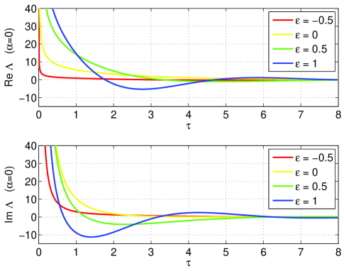
Figure 1: (Color online) The time dependence of the real (top) and imaginary (bottom) parts of the function $\Lambda$ in (47) which enters the quantum ${\mathrm{FFCF}}$ for an harmonic barrier in (46a). The graphs are for different values of the scaled energy $\epsilon$.

Equations (46a) and (47) yield an exact expression for the microcanonical quantum ${\mathrm{FFCF}}$ of the parabolic barrier system with Hamiltonian $(\hat{p}^{2}-\lambda^{2}\hat{q}^{2})/2$. The corresponding canonical version of the ${\mathrm{FFCF}}$, defined as

$${\overline{\mathcal{C}}_{\mathrm{QM}}}(\beta,t,a)={\mathrm{Tr}}\left\{e^{-\beta\hat{H}}\hat{F}e^{i\hat{H}t/\hbar}\hat{F}e^{-i\hat{H}t/\hbar}\right\}\,,$$ (48)

can be readily calculated for the case of $a=0$ by performing the bilateral Laplace transformation of (46a) which gives

$${\overline{\mathcal{C}}_{\mathrm{QM}}}(\beta,t,0) =\int_{-\infty}^{+\infty}dE\,e^{-\beta E}{\mathcal{C}_{\text{QM}}}(E,t,0)$$

$$=\frac{\lambda^{2}}{4\pi}\frac{\cosh(\lambda t_{c})\sinh(\lambda\hbar\beta/2)}{\left[\sinh^{2}(\lambda t_{c})+\cosh^{2}(\lambda\hbar\beta/2)\right]^{3/2}}$$ (49)

with $t_{c}=t-i\hbar\beta/2$. Here Eq. (45) with $A=C=0$ was used to calculate the integral over energy.

We note that Eq. (49) was originally obtained by Miller et al. Miller et al. (1983) by representing the ${\mathrm{FFCF}}$ in terms of the time evolution operator for the harmonic oscillator. However, to our knowledge, the explicit expression for the microcanonical ${\mathrm{FFCF}}$ in Eqs. (46a) and (47) has not been reported in the literature before.

In Fig. 1 the time dependence of the function $\Lambda$ in (47) is shown for different values of the scaled energy $\epsilon$. We note that $\Lambda$ and hence the microcanonical ${\mathrm{FFCF}}$ always diverge in the limit $t\to 0$ and depending on the energy shows more or less pronounced oscillations.

III.2 The short-time regime ($\lambda t\ll 1$)

For short times, $\tau\ll 1$, one can approximate the hyperbolic functions on the right-hand side of Eq. (46d) by their leading order Taylor expansions to obtain

$$\Omega {}_{\sigma}(\nu;\varepsilon,\tau,\alpha)$$

$$\simeq\alpha^{2}\big{(}\epsilon_{\sigma}^{2}\mathcal{D}_{2\nu}-4i\nu\epsilon_{\sigma}\mathcal{D}_{2\nu+1}+2\nu(2\nu+1)\mathcal{D}_{2\nu+2}\big{)}$$ (50)

with

$$\mathcal{D}_{\mu}(\tau,\alpha)=\exp\left(-i\alpha\tau\frac{\partial^{2}}{\partial\tau^{2}}\right)\frac{1}{\tau^{\mu}}\,.$$ (51)

As shown in Appendix B $\mathcal{D}_{\mu}$ in Eq. (51) can be written as

$$\mathcal{D}_{\mu}(\tau,\alpha)=e^{\gamma^{2}\!/4}\,D_{-\mu}(\gamma)\left(\frac{\gamma}{\tau}\right)^{\mu},\quad\gamma=\left(\frac{\tau}{2\alpha}e^{-i\pi/2}\right)^{1/2}\!.$$ (52)

Equations (46a-46c) together with Eqs. (50) and (52) provide an explicit expression for the ${\mathrm{FFCF}}$ at short times.

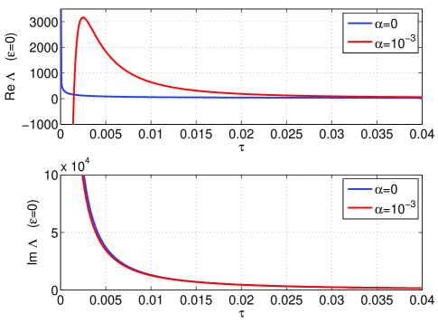
Figure 2: (Color online) Short time regime of the real (top) and imaginary (bottom) parts of the function $\Lambda$ which enters the quantum ${\mathrm{FFCF}}$ in (46a) (see Sec. III.2). The graphs are for different values of the scaled anharmonicity parameter $\alpha$ and all have energy zero.

Figure 2 compares the time decay of the dimensionless correlation function $\Lambda$ in the harmonic case ($\alpha=0$, blue lines), given by Eq. (47), and that in the anharmonic case ($\alpha=10^{-3}$, red lines), given by Eqs. (46b), (50), and (52). One sees that even for very small (but non-vanishing) values of the dimensionless anharmonicity parameter $\alpha$ the time dependence of the ${\mathrm{FFCF}}$ significantly differs from that of the corresponding harmonic problem. In fact, it is straightforward to show that as $\tau\rightarrow 0$ one has $\mathrm{Re}\,\Lambda\rightarrow+\infty$ for $\alpha=0$, while $\mathrm{Re}\,\Lambda\rightarrow-\infty$ for $\alpha>0$. The transition from the anharmonic case to the harmonic one takes place in a discontinuous manner: as $\alpha$ tends to zero the maximum of $\mathrm{Re}\,\Lambda$ (i.e., the peak of the red curve in the upper half of Fig. 2) becomes higher and sharper and approaches $\tau=0$ recovering the harmonic result (the monotonic blue curve in Fig. 2).

IV Conclusions

In this paper we have presented a method for computing classical and quantum flux-flux correlation functions for reactive systems with a potential barrier characterized by saddle type equilibria in phase space. The method is based on the normal form transformation of the system’s Hamiltonian in a vicinity of the saddle point.

In the classical case, the time dependence of the correlation function (with respect to a recrossing free dividing surface) is given by the $\delta$-function. While this form of the time dependence has been known in the theoretical chemistry community for some time, the contribution of the classical normal form theory is that it provides a dividing surface having the no-recrossing property that allows the computation of the pre-factor (essentially the flux through the dividing surface). No computation of trajectories is required to evaluate the flux-flux correlation function. The time integration to compute the rate becomes trivial.

In the quantum case, we showed that the problem of calculating the correlation function in a system with more than one degree-of-freedom reduces to an effective one degree-of-freedom problem. The Hamiltonian of this effective one degree-of-freedom system is obtained through the quantum normal form procedure. Finally, and most importantly, we derive (for the first time in the literature) an analytical expression for the flux-flux correlation function for the simplest anharmonic one-dimensional Hamiltonian in quantum normal form.

Appendix A Derivation of Eq. (45)

We begin our derivation of the formula, Eq. (45), by writing

$$\big{|}\Gamma(D+ix)\big{|}^{2}=\frac{\Gamma(2D)}{2^{2D}}\int_{-\infty}^{+\infty}dq\,\frac{e^{-iqx}}{\big{[}\cosh(q/2)\big{]}^{2D}}\,.$$ (53)

The integral representation given by Eq. (53) is readily obtained, e.g., from formula 5.13.2 in Ref. nis (2010). Then, denoting the left-hand side of Eq. (45) by $\mathcal{I}$ we get

$$\mathcal{I}= \frac{\Gamma(2D)}{2^{2D}}\int_{-\infty}^{+\infty}\frac{dq}{\big{[}\cosh(q/2)\big{]}^{2D}}$$

$$\times\int_{-\infty}^{+\infty}dx(1+Cx)^{2}e^{iAx^{2}-i(q+iB)x}\,.$$ (54)

The second integral in the right-hand side of Eq. (54) can be written as

$$\sum_{n=0}^{\infty}\frac{(iA)^{n}}{n!}\int_{-\infty}^{+\infty}dx\,x^{2n}(1+Cx)^{2}e^{-i(q+iB)x}\,.$$ (55)

Now, using

$$\int_{-\infty}^{+\infty}dxx^{n}e^{-i(q+iB)x}=2\pi i^{n}\delta^{(n)}(q+iB)\,,$$ (56)

with $\delta^{(n)}$ denoting the $n$th derivative of the delta function, and then, carrying out the $q$-integration in Eq. (55) we obtain

$$\mathcal{I}=2\pi \frac{\Gamma(2D)}{2^{2D}}\sum_{n=0}^{\infty}\frac{(-iA)^{n}}{n!}\frac{\partial^{2n}}{\partial q^{2n}}$$

$$\frac{\big{(}\cosh\frac{q}{2}+iCD\sinh\frac{q}{2}\big{)}^{2}+\frac{1}{2}C^{2}D}{\big{(}\cosh\frac{q}{2}\big{)}^{2D+2}}\Bigg{|}_{q=-iB}\!\!\!.$$ (57)

Finally, formally summing the series,

$$\sum_{n=0}^{\infty}\frac{(-iA)^{n}}{n!}\frac{\partial^{2n}}{\partial q^{2n}}\,f(q)=\exp\left(-iA\frac{\partial^{2}}{\partial q^{2}}\right)f(q)$$ (58)

with $f$ denoting an arbitrary function, and making the change $x=q/2$ we arrive at Eq. (45).

Appendix B Derivation of Eq. (52)

Taking into account the identity

$$\frac{1}{\tau^{\mu}}=\frac{1}{\Gamma(\mu)}\int_{0}^{\infty}ds\,s^{\mu-1}e^{-\tau s}$$ (59)

we rewrite Eq. (51) as

$$\mathcal{D}_{\mu}=\frac{1}{\Gamma(\mu)}\int_{0}^{\infty}ds\,s^{\mu-1}e^{-i\alpha\tau s^{2}-\tau s}\,.$$ (60)

Then, using formula 3.462.1 in Ref. Gradshteyn and Ryzhik (2000),

$$\int_{0}^{\infty} ds\,s^{\mu-1}e^{-As^{2}-Bs}$$

$$=\frac{\Gamma(\mu)}{(2A)^{\mu/2}}\exp\left(\frac{B^{2}}{8A}\right)D_{-\mu}\left(\frac{B}{\sqrt{2B}}\right)\,,$$ (61)

for $A=e^{i\pi/2}\alpha\tau$ and $B=\tau$ we arrive at Eq. (52).

References

- Miller et al. (1983) W. H. Miller, S. D. Schwartz, and J. W. Tromp, J. Chem. Phys., 79, 4889 (1983).
- Yamamoto (1960) T. Yamamoto, J. Chem. Phys., 33, 281 (1960).
- Miller (1974) W. H. Miller, J. Chem. Phys., 61, 1823 (1974).
- Wang et al. (1998) H. Wang, X. Sun, and W. H. Miller, J. Chem. Phys., 108, 9726 (1998).
- Ceotto et al. (2005) M. Ceotto, S. Yang, and W. H. Miller, J. Chem. Phys., 122, 044109 (2005).
- Venkataraman and Miller (2007) C. Venkataraman and W. H. Miller, J. Chem. Phys., 126, 094104 (2007).
- Miller (1998) W. H. Miller, Farad. Discuss., 110, 1 (1998a).
- Miller (1998) W. H. Miller, J. Phys. Chem. A, 102, 793 (1998b).
- Department of Energy (2007) Department of Energy, “Directing Matter and Energy: Five Challenges for Science and the Imagination. A Report from the Basic Energy Sciences Advisory Committee, US Department of Energy, December 20, 2007,” (2007).
- Miller (2008) W. H. Miller, in Physical Biology–From Atoms to Cells, Conference on Chemical Research, edited by K. K. Phua and A. Zewail (Imperial College Press, London, UK, 2008) pp. 505–525.
- Wiggins et al. (2001) S. Wiggins, L. Wiesenfeld, C. Jaffe, and T. Uzer, Phys. Rev. Lett., 86(24), 5478 (2001).
- Uzer et al. (2002) T. Uzer, C. Jaffe, J. Palacian, P. Yanguas, and S. Wiggins, Nonlinearity, 15, 957 (2002).
- Waalkens et al. (2004) H. Waalkens, A. Burbanks, and S. Wiggins, J. Chem. Phys., 121, 6207 (2004).
- Waalkens and Wiggins (2004) H. Waalkens and S. Wiggins, J. Phys. A, 37, L435 (2004).
- Wiggins (1994) S. Wiggins, Normally hyperbolic invariant manifolds in dynamical systems (Springer-Verlag, 1994).
- Schubert et al. (2006) R. Schubert, H. Waalkens, and S. Wiggins, Phys. Rev. Lett., 96, 218302 (2006).
- Waalkens et al. (2008) H. Waalkens, R. Schubert, and S. Wiggins, Nonlinearity, 21, R1 (2008).
- (18) A. Goussev, R. Schubert, H. Waalkens, and S. Wiggins, “Quantum theory of reactive scattering in phase space,” To appear in Advances in Quantum Chemistry, e-print: arXiv:1004.5017.
- Tromp and Miller (1987) J. W. Tromp and W. H. Miller, Faraday Discuss. Chem. Soc., 84, 441 (1987).
- Chruściński (2003) D. Chruściński, J. Math. Phys., 44, 3718 (2003a).
- Chruściński (2003) D. Chruściński, J. Math. Phys., 45, 841 (2003b).
- Abramowitz and Stegun (1965) M. Abramowitz and I. A. Stegun, Handbook of Mathematical Functions with Formulas, Graphs, and Mathematical Tables (Dover, New York, 1965) ISBN 0-486-61272-4.
- nis (2010) “Digital library of mathematical functions,” National Institute of Standards and Technology, http://dlmf.nist.gov/ (2010).
- Gradshteyn and Ryzhik (2000) I. S. Gradshteyn and I. M. Ryzhik, Table of Integrals, Series and Products, edited by A. Jeffrey and D. Zwillinger (Academic Press Inc.; 6th edition, 2000).